Article

Time-Allocation Adaptive Data Rate: An Innovative Time-Managed Algorithm for Enhanced Long-Range Wide-Area Network Performance

1
Science and Technology on Electronic Test and Measurement Laboratory, North University of China, Taiyuan 030051, China
2
College of Software, Shanxi Agricultural University, Jinzhong 030801, China
*
Author to whom correspondence should be addressed.
Electronics 2024, 13(2), 434; https://doi.org/10.3390/electronics13020434
Submission received: 15 December 2023 / Revised: 17 January 2024 / Accepted: 18 January 2024 / Published: 20 January 2024

Abstract

:
Currently, a variety of Low-Power Wide-Area Network (LPWAN) technologies offer diverse solutions for long-distance communication. Among these, Long-Range Wide-Area Network (LoRaWAN) has garnered considerable attention for its widespread applications in the Internet of Things (IoT). Nevertheless, LoRaWAN still faces the challenge of channel collisions when managing dense node communications, a significant bottleneck to its performance. Addressing this issue, this study has developed a novel “time allocation adaptive Data Rate” (TA-ADR) algorithm for network servers. This algorithm dynamically adjusts the spreading factor (SF) and transmission power (TP) of LoRa (Long Range) nodes and intelligently schedules transmission times, effectively reducing the risk of data collisions on the same frequency channel and significantly enhancing data transmission efficiency. Simulations in a dense LoRaWAN network environment, encompassing 1000 nodes within a 480 m × 480 m range, demonstrate that compared to the ADR+ algorithm, our proposed algorithm achieves substantial improvements of approximately 30.35% in data transmission rate, 24.57% in energy consumption, and 31.25% in average network throughput.

1. Introduction

In today’s digital landscape, the Internet of Things (IoT) has become a pivotal force in bridging the gap between the virtual and physical worlds, driving connectivity across a myriad of devices [1]. With the exponential growth of IoT endpoints, conventional wireless networks are hitting their limits in scalability and energy efficiency [2]. This has prompted a shift toward more sustainable, low-energy, and expansive communication frameworks. Within this paradigm, Low-Power Wide-Area Networks (LPWANs) stand out as a beacon of IoT connectivity, offering a trifecta of benefits: minimal power requirements, extensive coverage, and economical operation. As a member of the numerous Low-Power Wide-Area Network (LPWAN) technologies, LoRaWAN is widely used in modern smart cities due to its advantages such as simple and flexible network formation, operation in unlicensed frequency bands, and the ability to communicate remotely with extremely low power consumption. It is considered one of the most promising LPWAN technologies today [3,4,5] and is applied in areas like monitoring water consumption in urban buildings and checking [6] the structural health of buildings [7].
LoRaWAN is a Media Access Control (MAC) protocol built on top of the LoRa (Long-Range) physical layer. LoRa itself is a wireless modulation method at the physical layer, based on Chirp Spread Spectrum (CSS) [8] technology, and is focused on providing long-distance, low-power wireless transmission. The core advantage of LoRa technology lies in its ability to achieve low data rate communication over long distances while maintaining low energy consumption. In contrast, LoRaWAN defines how to establish a complete network on the foundation of LoRa, encompassing features like device addressing, encrypted communication, data rate management, and multiple access. To facilitate interoperability among LoRa devices from different manufacturers and to provide better support for the diversity and scalability of LoRa technology in IoT applications, the LoRa Alliance introduced the standardized LoRaWAN communication protocol in 2015. This protocol not only promotes compatibility among LoRa devices from various suppliers but also enhances the functionality and reliability of the entire LoRa network.
The classical LoRaWAN follows a star network topology, primarily consisting of end devices, gateways, and a network server, as shown in Figure 1. The end devices are IoT terminal nodes responsible for data collection and communication with the gateways. Gateways serve as intermediate devices, connecting the end devices to the network server and handling the reception and forwarding of data from the end devices. The network server is the core of the LoRaWAN network, responsible for managing and coordinating communication between end devices and gateways, as well as handling functions such as data transmission, device authentication, and security [9].
The LoRaWAN standard protocol defines three classes of end devices, Class A, Class B, and Class C, to meet the power and latency requirements of different scenarios [10,11]. Among them, Class A is the most common and basic device class that all LoRa devices must support. It has the lowest power consumption and the simplest communication mode. Its operation is illustrated in Figure 2. In Class A mode, the end devices actively send data packets based on their own needs. After a certain airtime delay, these packets are received by one or multiple gateways. Following the completion of an uplink transmission, the device pauses for a period (Delay 1). During this time, the gateway sends downlink data to the end device, based on the frequency and data rate of the previous uplink transmission. After each data transmission, the end device sequentially opens two short receive windows, with their opening times determined by the end of the transmission. If the end device successfully receives data during the first receive window, it does not open the second receive window. If not, after the first window closes and following another period (Delay 2), the device opens the second receive window to continue receiving potential data. Since the gateway cannot ascertain whether the end device has actually opened the receive window, it proceeds to send data during the pre-scheduled periods of both receive windows.
The Adaptive Data Rate (ADR) feature in the LoRaWAN protocol plays a crucial role in optimizing communication efficiency by dynamically adjusting two key parameters: spreading factor and transmit power. These parameters help regulate network capacity, coverage, power consumption, and device lifespan. Increasing SF levels enhances interference resistance and sensitivity, widening coverage but at the cost of lower data rates and increased energy requirements. Conversely, TP directly impacts communication range and energy consumption. To balance these factors, LoRaWAN employs a standard ADR algorithm to harmonize SF and TP, thereby improving overall network throughput [10]. Additionally, the quasi-orthogonal nature of different SFs in LoRaWAN allows for nearly interference-free transmissions on the same bandwidth when the SFs are different [12]. However, significant signal interference occurs between LoRa nodes using the same SF. However, as the density of nodes increases, more nodes with the same SF transmitting at the same time lead to escalated data collisions, significantly reducing the data transmission success rate.
To address this challenge, our proposed Time-Allocation Adaptive Data Rate (TA-ADR) algorithm innovates by calibrating the adjustment steps for SF and TP. It introduces the concept of transmission time intervals for LoRa nodes, allocating appropriate time slots for nodes with the same SF to transmit data, thereby reducing the risk of conflicts and enhancing the transmission success rate.
The rest of this article is structured as follows. In Section 2, we present an overview of the related work and introduce the main contributions of our study. Section 3 describes the flow of the ADR+ algorithm and the optimized TA-ADR algorithm. Section 4 introduces the simulation configuration and gives the analysis of the results after simulation. The conclusion of this paper is given in Section 5.

2. Related Work

The ADR algorithm, as a fundamental feature in the LoRaWAN protocol, is a key advantage and has received extensive attention from many research teams. Several research teams have focused on optimizing the ADR algorithm to adapt to different application scenarios and network requirements, proposing a series of corresponding improvement methods.
Slabicki et al. pointed out in the literature [13] that the basic ADR algorithm mentioned in the LoRaWAN standard protocol is to select the maximum signal-to-noise ratio in the last 20 packets as the calculation basis, but this method is too optimistic in a noisy channel. Therefore, they simply modified the ADR algorithm. In the proposed ADR+ algorithm, the average value of the SNR of the latest packet is used as the basis for the subsequent calculation, which improves the performance of ADR algorithm in noisy channels.
In reference [14], Babaki et al. introduced the Ordered Weighted Averaging (OWA) operator to optimize the ADR algorithm for accurately demodulating the suitable spreading factor based on the current channel conditions and external environment. This algorithm improves the transmission success rate and achieves almost the same energy consumption as other ADR algorithms, even in dense LoRa networks and high channel noise.
Reference [15] proposes a new and more efficient dynamic ADR algorithm called ND-ADR (New-Dynamic Adaptive Data Rate Algorithm). This algorithm introduces RSSI in addition to the basic ADR algorithm’s selection of SF based solely on the maximum SNR value. By combining the average values of RSSI and SNR, ND-ADR dynamically adjusts the number of SNR values considered (denoted as “n”). Initially set to three frames, the value of “n” is dynamically increased based on certain conditions. This allows the server to quickly adapt to changes in the external environment, effectively addressing communication quality issues and high packet loss rates in mobile terminal devices operating in harsh environments.
In reference [16], the authors build upon the ADR+ algorithm by introducing an energy efficiency controller α, which is related to the total energy consumption of all nodes. The algorithm multiplies the average SNR value from the most recent 20 packets by α and then gradually decreases α from 1 in steps of 0.1. This approach aims to find the optimal α value that minimizes network energy consumption without compromising data delivery rates. The simulation results presented in the reference demonstrate that this algorithm outperforms the ADR+ algorithm in terms of energy consumption and data delivery rates.
In reference [17], Marini et al. propose a new ADR algorithm for LoRaWAN networks called CA-ADR (Collision-Aware ADR). This algorithm takes into account the collision probability at the MAC layer of the network. When allocating data rates, it minimizes the collision probability while maintaining controllable link performance by considering the set of nodes in the entire network. The feasibility of both cloud computing and fog computing architectures is also validated. The results demonstrate that the fog computing-based architecture is feasible and reduces end-to-end transmission latency.
In reference [18], Jeon et al. present a simple and energy-efficient uplink transmission rate control scheme for LoRaWAN. The aim is to support efficient communication for a large number of IoT devices over a wide area. This scheme enables devices to increase or decrease the transmission rate based on the changing link quality. It introduces a ping-pong mechanism to avoid frequent rate changes. Through modeling and simulation comparisons, the results show that this scheme outperforms other approaches in terms of transmission success rate, effective transmission rate, frame transmission delay, and energy consumption.
In reference [19], Anwar et al. discovered that fixed SF allocations are no longer efficient in LoRaWAN when the end devices (EDs) are in motion. The link conditions between the EDs and gateways change abruptly, resulting in significant packet loss and increased retransmission attempts. To address this issue, they propose a resource management ADR (RM-ADR) scheme that considers both packet transmission information and received power. The research findings indicate that in a mobile LoRaWAN network environment, RM-ADR achieves faster convergence time by reducing packet loss and retransmission attempts.
Reference [20] mentioned an EE-LoRa for spread spectrum factor selection and power control in multi-gateway LoRaWAN networks. The author first optimized the energy efficiency of the network, and then applied power control to minimize the transmit power of nodes while maintaining the reliability of communication.
In reference [21], Cuomo et al. proposed two LoRa spread spectrum channel allocation algorithms to solve the problems existing in the ADR algorithm allocation mechanism of LoRaWAN. Scenario 1 (EXPLoRa-SF) uses a heuristic algorithm to evenly allocate SFs to these nodes, with the same number of LoRa nodes for each spread spectrum factor. Scenario 2 (EXPLoRa-AT) is used to fairly distribute broadcast time among network nodes so that the various SFs transmit data at the same time.
We summarize the features of the ADR algorithms mentioned in Table 1.
Compared to the ADR algorithms proposed in the existing literature, our TA-ADR algorithm incorporates a time scheduling strategy, allowing for the allocation of communication windows within the LoRaWAN network to reduce channel conflicts among nodes with the same SF. This approach not only enhances the success rate of data transmission but also optimizes the network’s energy consumption efficiency. Here are the primary contributions of our study:
(1)
The TA-ADR algorithm diminishes channel conflicts by distributing non-overlapping communication time windows among nodes, thereby improving the data delivery rate and network throughput.
(2)
The TA-ADR algorithm adapts the timetable to changes in node density, particularly as the number of nodes increases, enabling better management of communication loads.

3. Introduction and Optimization of ADR+ Algorithm

3.1. Standard ADR Algorithm and ADR+ Algorithm

In this section, the speed regulation mechanism of the ADR algorithm is introduced, and then we describe the standard ADR algorithm and ADR+ algorithm. Finally, the algorithm of the SF and TP adjustment stage is optimized on the basis of the ADR+ algorithm, and the optimization process is described in detail.
The ADR mechanism can be divided into two parts: the network server (NS)-side algorithm is responsible for increasing the data transmission rate of end nodes, while the end node (ED)-side algorithm is responsible for decreasing the data transmission rate of end nodes. The ED-side algorithm for ADR is defined by the LoRa Alliance, while developers can choose basic ADR algorithms or configure their own algorithms for the NS side [15]. Additionally, the NS is located at the core of the network, allowing it to access global information. This enables the NS-side algorithm to dynamically adjust SF and TP of end nodes based on global information, leading to better optimization of network performance compared to node-side algorithms. The ADR algorithm in the LoRaWAN standard protocol includes both the ED-side algorithm and the NS-side algorithm. The ED-side algorithm relies on acknowledge character (ACK) feedback to determine if the data transmission is successful. If the node does not receive an acknowledgment from the gateway within two receiving windows, it considers the data transmission as failed and activates the retransmission mechanism. It automatically reduces the data transmission rate before retransmitting the data. The NS-side algorithm determines the link quality based on the signal-to-noise ratio ( S N R ) of the recently received data and adjusts the SF and TP accordingly. The ADR+ algorithm, compared to the ADR algorithm, only modifies the NS-side algorithm while keeping the node-side algorithm unchanged. Algorithm 1 describes the implementation steps of the NS-side ADR+ algorithm [
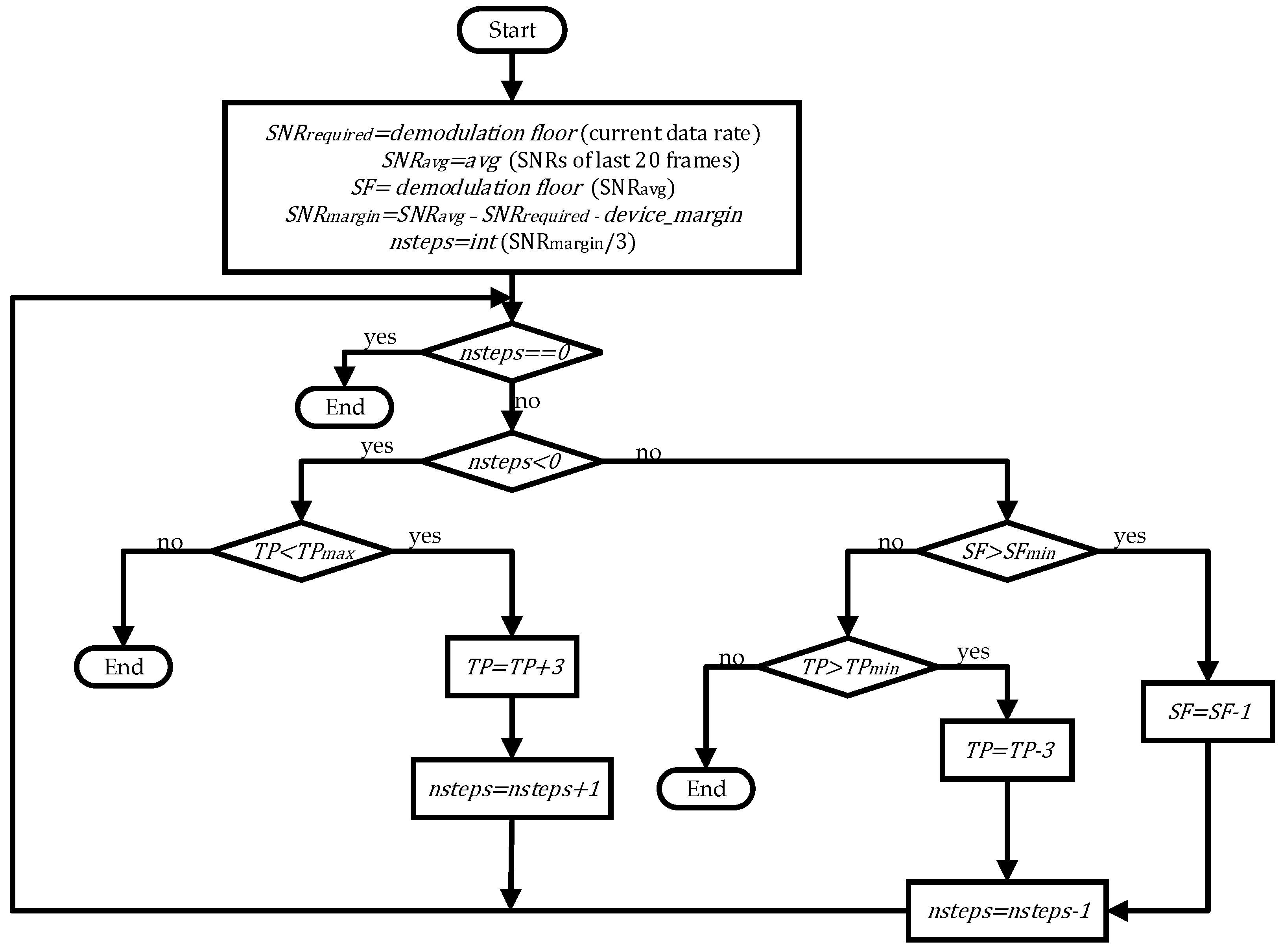
14]. In Algorithm 1, the input SF value ranges from 7 to 12 in steps of 1, and the input TP value ranges from 2 to 14 in steps of 3. It involves calculating the required SNR ( S N R r e q u i r e d ) based on the current SF, averaging the SNR of the latest received 20 data packets to obtain S N R a v g , determining the appropriate SF based on S N R a v g , and then computing the SNR margin ( S N R m a r g i n ) and the adjustment steps ( n s t e p s ) using Equations (1) and (2):
S N R m a r g i n = S N R   a v g S N R   r e q u i r e d d e v i c e m a r g i n
n s t e p s = i n t ( S N R m a r g i n / 3 )
Ultimately, through iteration, the values of SF and TP are gradually adjusted until certain conditions are met, and then the adjusted values of SF and TP are output. Table 2 lists the minimum SNR required for different SFs. If the SNR margin ( S N R m a r g i n ) is positive, it indicates that the current channel quality is good, and the node can increase the data rate or decrease the transmission power to reduce power consumption and extend the node’s battery life. If the SNR margin is negative, it indicates that the node is currently using a transmission power that is too low, resulting in a low SNR for the uplink signal. Therefore, it is necessary to increase the transmission power or decrease the data rate.
Algorithm 1 NS ADR+ Algorithm
Input: S F 7 , 12 , T P 2 , 14 ,
Output: S F and T P
  • S N R r e q u i r e d = d e m o d u l a t i o n   f l o o r   ( c u r r e n t   d a t a   r a t e )
  • S N R a v g = a v g   ( S N R s   o f   l a s t   20   f r a m e s )
  • S F = d e m o d u l a t i o n   f l o o r   ( S N R a v g )
  • S N R m a r g i n = S N R a v g S N R r e q u i r e d d e v i c e _ m a r g i n
  • n s t e p s = i n t ( S N R m a r g i n / 3 )
  • w h i l e   n s t e p s   >   0   a n d   S F > S F m i n
                S F = S F 1
                n s t e p s = n s t e p 1
      e n d   w h i l e
7.
w h i l e   n s t e p s > 0   a n d   T P > T P m i n
                T = T P 3
                n s t e p s = n s t e p s 1
      e n d     w h i l e
8.
w h i l e   n s t e p s < 0   a n d   T P < T P m a x
                T P = T P + 3
                n s t e p s = n s t e p s + 1
      e n d   w h i l e
The flowchart of the ADR+ algorithm is presented in Figure 3.

3.2. Algorithm Optimization

In this section, we will introduce the idea of algorithm optimization and the optimized algorithm.
The ADR+ algorithm has powerful capabilities in controlling data rates, which can improve the communication success rate and reduce the overall network energy consumption to some extent. However, from the ADR+ algorithm flow, it is evident that the ADR+ algorithm always starts by changing the spreading factor and tends to decrease it. In a network with a large number of deployed LoRa nodes, this can lead to numerous nodes operating on the same spreading channel, resulting in severe data collisions, increased triggering of the node’s retransmission mechanism, and inevitably increasing network energy consumption while reducing the communication success rate.
To address these issues, we propose the communication time algorithm to allocate signal transmission times for nodes with the same spreading factor. The message types in LoRaWAN are divided into uplink messages and downlink messages. The data packet structure of uplink messages mainly consists of five parts as shown in Figure 4: Preamble, PHDR (Physical Header), PHDR_CRC (Physical Header Cyclic Redundancy Check), PHYPayload (Physical Payload), and CRC (Cyclic Redundancy Check). The PHDR_CRC is the Cyclic Redundancy Check for the PHDR, which is used to detect errors in the header information. The CRC is for the PHYPayload, ensuring the integrity of the data payload [10].
The transmission time of a LoRaWAN data packet is composed of the transmission time of the preamble and the transmission time of the payload. The transmission time of the preamble is determined by the symbol effective length N P r e a m b l e and the time to send a single symbol T s , where T s is related to the symbol rate R s of LoRa. The specific calculation formula is as follows:
R s = B W 2 S F
T s = 1 R s
T P r e a m b l e = N P r e a m b l e + 4.25 × T s
Here, B W represents bandwidth, and S F represents spreading factor.
The transmission time of the payload is related to the selected header type. In explicit header mode, the header contains information such as payload length, forward error correction rate, and whether CRC is used. In implicit header mode, the payload bytes, forward error correction rate, and CRC need to be manually set. The number of payload symbols ( N P a y l o a d ) is calculated as follows:
N P a y l o a d = 8 + max c e i l 8 P L 4 S F + 28 + 16 20 H 4 S F 2 D E C R + 4 , 0
where P L is the number of bytes in the payload. H represents the selected header type, where H = 0 indicates explicit header mode and H = 1 indicates implicit header mode. D E represents whether low data rate optimization is used during data transmission, where D E = 1 indicates it is used and D E = 0 indicates it is not used. max ( ) denotes the maximum value function, and c e i l ( ) represents the ceiling function for rounding up.
After obtaining the number of payload symbols, the formula to calculate the transmission time of the payload ( T P a y l o a d ) is defined as:
T P a y l o a d = N P a y l o a d × T s
Finally, by adding the transmission time of the preamble and the transmission time of the payload, we can determine the transmission time of the LoRa data packet ( T P a c k e t ):
T P a c k e t = T P e a m b l e + T P a y l o a d
From the derivation of the above data packet transmission time formulas, we can see that the factors affecting the data packet transmission time include B W , S F , C R , N P r e a m b l e , P L , header type, and whether low data rate optimization is used. In this article, our algorithm only dynamically adjusts the SF and TP of the LoRa node. Therefore, we preset the variables W , C R , N P r e a m b l e , header type, and whether low data rate optimization is used. We set B W to 125 kHz, C R to 1, N P r e a m b l e to 8, P L to 23 bytes, H = 0 for explicit header, and D E = 0 for not using the low data rate optimization configuration. By using the formulas, we can calculate the number of payload symbols N P r e a m b l e and the transmission time T P a c k e t of the LoRa data packet for different spreading factors, as shown in Table 3.
From Table 3, it can be observed that if a LoRa node uses SF12 to transmit a data packet, then within the corresponding time, 21 LoRa nodes using SF7 can complete the transmission of one data packet. Next, we established a communication time algorithm for all nodes based on their channel, spreading factor, and node number. We calculated the communication time interval t i S F which characterizes the time interval from the beginning to the end of data transmission by a LoRa node i at the SF, where the time occupied by a spreading factor channel is denoted as T S F , such as T 7 = 61.696   m s . The time interval between node communications is denoted as T S F , such as T 7 = 123.392   m s . Assuming the starting time of the first node is t 0 , the formula to determine the interval of t i S F is defined as:
T S F = 2     T S F
t i S F t 0 + T S F + T S F i 1 ,   t 0 + T S F i + T S F i 1
Based on the time interval t i S F , a new algorithm called TA-ADR (Time Slot Adaptive Data Rate) is proposed. The algorithm flow of TA-ADR is detailed in Algorithm 2.
Algorithm 2 NS TA-ADR Algorithm
Input: S F 7 , 12 ;     T P 2 , 14 ; Time range T of the current node; Timetable T i S F of communication of all nodes in LoRa gateway.
Output:   S F ,   T P and update timetable T i S F of all node communications for all spread spectrum channels of LoRa Gateway.
  • S N R r e q u i r e d = d e m o d u l a t i o n   f l o o r   ( c u r r e n t   d a t a   r a t e )
  • S N R a v g = a v g   ( S N R s   o f   l a s t   20   f r a m e s )
  • S F = d e m o d u l a t i o n   f l o o r   ( S N R a v g )
  • S N R m a r g i n = S N R a v g S N R r e q u i r e d d e v i c e _ m a r g i n
  • n s t e p s = i n t ( S N R m a r g i n / 3 )
  • w h i l e   n s t e p s   >   0   & &   T P   >   T P m i n   D o
                T P = T P 3
                n s t e p s = n s t e p s 1
     e n d   w h i l e
7.
i f   n s t e p s   >   0   a n d   S F n s t e p s S F m i n
                i f   T t i S F n s t e p s = =
                       S F = S F n s t e p s , n s t e p s = 0 ;
                e l s e   S F = S F n s t e p s 1 , k = 1 ;
                       w h i l e   T t i S F ! =   a n d   S F > S F m i n
                                S F = S F 1 , k = k + 1 ;
                                i f   T t i S F = =   a n d   T P + k     3 T P m a x
                                    T P = T P + k     3 , n s t e p s = 0 ;
                                    b r e a k ;
                   e n d   w h i l e
       e n d   i f
8.
w h i l e   n s t e p s < 0   a n d   T P < T P m a x D o
                T P = T P + 3
                n s t e p s = n s t e p s + 1
       e n d   w h i l e
9.
i f   n s t e p s < 0   a n d   S F n s t e p s S F m a x
                i f   T t i S F n s t e p s = =
                      S F = S F n s t e p s , n s t e p s = 0 ;
                e l s e   S F = S F n s t e p s 1 , k = 1 ;
                      w h i l e   T t i S F ! =   a n d   S F < S F m a x
                              S F = S F + 1 , k = k + 1 ;
                              i f   T t i S F = =   a n d   T P + k     3 T P m i n
                                      T P = T P k     3 , n s t e p s = 0 ;
                                      b r e a k ;
                e n d   w h i l e
      e n d   i f

3.3. Algorithm Implementation

In Section 3.2 of our paper, we delved into a novel ADR management algorithm, dubbed the Time-Allocation Adaptive Data Rate algorithm. This algorithm is designed to optimize data transmission and significantly reduce conflicts between nodes on the same frequency channel using the same SF. This section will elaborate on the details of implementing the TA-ADR algorithm.
The input parameters for the TA-ADR algorithm include the SF range of the current node, the TP range, the time range T of nodes that need to be optimized, and the communication schedule T i S F of all nodes within the LoRa gateway. The output of the algorithm is the adjusted SF and TP values, along with an updated communication schedule for all nodes across all spread spectrum channels. To illustrate the relationship between T , t i S F , and T i S F , let us consider an example in a LoRaWAN network with six LoRa nodes, all having a TP of 2 dBm. Among these, three nodes use a SF of 7, while the other three use SF8, and the initial send time is 0 s. Therefore, the communication time intervals for these six nodes are t 1 S F 7 [ 0   s , 0.063   s ] , t 2 S F 7 [ 0.189   s , 0.252   s ] , t 3 S F 7 [ 0.378   s , 0.441   s ] , t 1 S F 8 [ 0   s , 0.114   s ] , t 2 S F 8 [ 0.342   s , 0.456   s ] , and t 3 S F 8 [ 0.684   s , 0.798   s ] , respectively. From this, we can derive the theoretical communication timetable T i S F for these nodes, as presented in Table 4.
After the nodes 2 and 3 using SF8 transmit their data, the NS calculates that these nodes have S N R m a r g i n with both having an n s t e p s of 1. Therefore, NS optimizes the parameters for these nodes under SF8 using Algorithm 2. For node 2 under SF8 (with T being t 2 S F 8 ), after evaluating intersections with t i S F 7   ( i = 1 , 2 , 3 ) , it is found that T intersects with t 3 S F 7 , indicating that node 2 should maintain its original settings. For node 3 under SF8 (with T being t 3 S F 8 ), no intersections are found with t i S F 7 ( i = 1 , 2 , 3 ) , suggesting the time slot under SF7 is available. Thus, NS sends frame information containing the adjusted SF value and the new communication interval to node 3 during its receive window. Node 3 then resets its parameters accordingly. The updated communication timetable T i S F is displayed in Table 5.
Next, the parameter calculation and cyclic part of algorithm 2 are discussed. Initially, the algorithm calculates the minimum SNR required ( S N R r e q u i r e d ) for the current SF, and computes the average SNR ( S N R a v g ) from the last 20 frames of data. Then, it adjusts the SF based on the S N R a v g . Then, the algorithm calculates the SNR margin ( S N R m a r g i n ), which is the difference between the average SNR and the required SNR, minus the device margin ( d e v i c e _ m a r g i n ). This SNR margin is then divided by 3 to determine the number of adjustment steps ( n s t e p s ). Then, the loop is entered; if n s t e p s is greater than 0, indicating that the SNR is higher than required, the algorithm attempts to reduce the TP to save energy. For each reduction in TP (by 3 dB each time), n s t e p s is decreased by 1, until TP reaches the minimum value or n s t e p s becomes 0. If there are remaining n s t e p s after reducing TP, the algorithm tries to decrease the SF. It first checks if lowering the SF would cause a conflict with the communication schedule of other nodes. If there is no conflict, SF is reduced, and n s t e p s is set to 0. If there is a conflict, the algorithm further decreases SF (by 1 each time), and for each decrease in SF, TP is increased by 3 dB, until a conflict-free configuration is found or SF is lowered to its minimum value. If the original nsteps is less than 0, indicating that the SNR is lower than required, the algorithm attempts to increase TP to improve signal quality. For each increase in TP (by 3 dB each time), n s t e p s is incremented by 1, until TP reaches its maximum value or nsteps becomes 0. If nsteps is still less than 0 after increasing TP, the algorithm tries to increase SF. Similarly, it checks for conflicts with the schedule after increasing SF, and if there is a conflict, it continues to increase SF (by 1 each time), and for each increase in SF, TP is decreased by 3 dB, until a conflict-free configuration is found or SF is increased to its maximum value.
It is important to emphasize that our proposed TA-ADR algorithm is implemented on the NS end. All logic and computational operations are performed internally within the NS, sparing the LoRa nodes any additional burden. The NS, after processing through Algorithm 2, sends the optimized SF, TP, transmission time, and the addresses of the specific nodes needing optimization to the gateway. The gateway then conveys this information to the respective nodes, which adjust their parameters and transmission times upon receipt. Additionally, to achieve time synchronization among the nodes, we make the LoRaWAN gateways periodically broadcast time stamp updates to ensure all LoRa nodes are precisely synchronized.

4. Simulation and Results

In this section, we divide our discussion into two parts: simulation parameter settings and result analysis. In the simulation parameter settings section, we present the path loss model used in the LoRaWAN network, as well as the topology, simulation range, and simulation parameters. The result analysis section provides comparative graphs of three algorithms in the LoRaWAN network and elaborates on the advantages of the TA-ADR algorithm.

4.1. Simulation Parameter Settings

In this network simulation, we used the log-normal shadowing path loss model [15] to simulate the path loss caused by attenuation and shadowing when the signal propagates through the air. The mathematical model is defined as follows:
L p d i = L p d 0 + 10 γ lg d i / d 0 + X σ
where L p d 0 represents the average path loss at the reference distance d 0 , measured in d B . d i is the distance from node i to the gateway. γ is the path loss exponent. X σ ( d B ) is a zero-mean Gaussian random variable with standard deviation σ .
The received signal power P r , i d can be obtained by subtracting the path loss P t , i from the transmit power L p ( d ) of node i [21]:
P r , i d = P t , i L p ( d i )
All LoRa nodes in the simulation are initialized in Class A transmission mode. The region parameters and path loss parameters are given in Reference [14], where the simulation area size is 480   m × 480   m and the path loss parameters d 0 , L p d 0 , γ , and σ are provided in Table 6.
According to the predefined network parameters in Table 7, we conducted simulations of LoRa networks using the FLoRa framework in the OMNeT++ platform. We evaluated the performance of three different ADR algorithms in an urban scenario. The LoRa network adopts a star network topology with the gateway placed at the center, as shown in Figure 5. The nodes are uniformly distributed around the gateway.
Each simulation runs for a duration of 24 h. In the network, each node sends only one data packet at a time (with a payload size of 23 bytes), and nodes with the same SF will wait for a time interval of 2     T S F before sending again. All LoRa nodes periodically send a round of information. The energy consumption of LoRa nodes comes from three states (send, receive, and sleep). Node transmission power consumption depends on node level and instantaneous current value during transmission. The current of the node in receive and sleep mode was obtained from the Semtech SX1272 data manual, and the operating voltage was 3.3   V [23].
Finally, we assessed the performance of the three schemes based on the following three parameters:
Energy consumption ( m J ): Defined as the total energy consumed by all nodes in the LoRaWAN network divided by the total number of data packets successfully received by the gateway.
Packet delivery rate ( % ): Defined as the total number of data packets successfully received by the LoRaWAN network server divided by the total number of data packets sent by all nodes.
Throughput ( b p s ): Defined as the amount of data successfully transmitted per second in the LoRaWAN network.

4.2. Interpretation of Result

From Figure 6a,b, it can be observed that as the number of nodes in the LoRaWAN network increases, the energy efficiency and the packet delivery rate decreases. It is evident that the TA-ADR algorithm performs better compared to the other two algorithms, and its performance advantage becomes even more significant as the number of nodes increases.
At a node count of 200, the ADR+ algorithm reduces energy consumption by approximately 2.73% compared to the ADR algorithm, while the TA-ADR algorithm reduces energy consumption by approximately 7.63% compared to the ADR algorithm, and by approximately 5.03% compared to ADR+. At a node count of 1000, the ADR+ algorithm reduces energy consumption by approximately 37.74% compared to the ADR algorithm, while the TA-ADR algorithm reduces energy consumption by approximately 53.04% compared to the ADR algorithm, and by approximately 24.57% compared to ADR+. This is because the ADR algorithm, which selects the maximum SNR value for SF decoding, is overly optimistic. In a noisy channel, the ADR algorithm is prone to selecting a high SNR value for decoding, resulting in a lower SF being decoded. In contrast, the ADR+ algorithm uses the average SNR value as a reference, resulting in more accurate SF decoding. However, in the subsequent adjustment steps, both algorithms prioritize assigning lower spreading factors to nodes. As a result, in the simulation scenario, most nodes under these algorithms transmit data with smaller SF, leading to data collisions and reduced data delivery. Nodes that fail to transmit trigger retransmissions, further increasing energy consumption.
In Figure 7, we present a statistical analysis of the final SF allocation for 1000 LoRa nodes under the three ADR algorithms. The results show that under the ADR algorithm, 643 nodes are assigned SF7 and 269 nodes are assigned SF8. Under the ADR+ algorithm, 503 nodes are assigned SF7 and 406 nodes are assigned SF8. In contrast, the TA-ADR algorithm assigns nodes almost equally in decreasing order of SFs, with an approximately 50% reduction in the number of nodes for each SF. Based on the propagation time of each SF in the 125   k H z bandwidth channel, as calculated in Table 2, when a node uses a higher SF to transmit a data packet, approximately two nodes using lower SFs can transmit data consecutively within that time frame. Therefore, when the spreading channel is fully utilized, the number of nodes using lower SFs should be approximately twice the number of nodes using higher SFs.
Although the TA-ADR algorithm, like the other two algorithms, prioritizes assigning lower spreading factors to LoRa nodes in subsequent SF adjustments, it allocates nodes with the same SF to different time slots for data transmission. When the low spread spectrum is fully allocated, it continues to allocate LoRa nodes to unused higher spreading channels and correspondingly reduces the TP of that node. This ensures that multiple LoRa nodes with the same SF do not transmit data in the same time slot, reducing the probability of data collisions and improving data delivery rates while reducing the number of node retransmissions. The results in Figure 6b further demonstrate that the LoRaWAN network under the TA-ADR algorithm exhibits superior packet delivery ratio (PDR) performance. On average, the PDR under the TA-ADR algorithm is approximately 30.35% higher than that under the ADR+ algorithm and approximately 59.54% higher than that under the ADR algorithm.
Finally, in order to more intuitively reflect the ability of nodes in the LoRaWAN network to transmit data under the TA-ADR algorithm, we selected the statistical data of the network throughput changes over time during the period from 16 h to the end of the simulation to display in Figure 8, and calculated the average value of throughput, which is given in Table 8. The average network throughput of the TA-ADR algorithm is about 31.25% higher than that of the ADR+ algorithm, and 48.65% higher than that of the ADR algorithm, which further proves the advantages of the TA-ADR algorithm.

5. Conclusions and Prospects

5.1. Conclusions

In this study, we propose an NS ADR algorithm for dynamically adjusting the SF and TP of LoRa nodes in dense LoRaWAN networks. The algorithm introduces the concept of time intervals, denoted as t i S F , for node transmissions. Its objective is to allocate independent time intervals to each node as much as possible, thereby mitigating data collision issues in densely populated scenarios. Through network simulations of LoRaWAN networks, we evaluated the performance of this algorithm and compared it with other algorithms. The results demonstrate that our proposed TA-ADR algorithm outperforms the comparison algorithms in terms of energy consumption, packet delivery rate, and throughput.

5.2. Deficiencies and Prospects

The optimal application scenario for the TA-ADR algorithm is primarily limited to network environments with deterministic and periodic traffic patterns. This limitation stems from the core principle of the TA-ADR algorithm, which involves pre-planning communication schedules for nodes within the network. In environments characterized by non-deterministic or non-periodic traffic patterns, the communication behavior of nodes may be random or unpredictable. Under such circumstances, the pre-planned communication schedules may not accurately reflect the actual communication needs of the nodes, leading to reduced communication efficiency. With the increase in the noise level in the environment, the effectiveness of the TA-ADR algorithm will become weaker and weaker, but it is still better than the other two algorithms. Therefore, in future work, exploring ways to improve the TA-ADR algorithm to better adapt to diverse traffic patterns will be an important research direction.

Author Contributions

Conceptualization, K.W. (Kunzhu Wang); methodology, K.W. (Kunzhu Wang); software, K.W. (Kunzhu Wang) and K.W. (Kun Wang); data analysis, K.W. (Kunzhu Wang) and K.W. (Kun Wang); investigation, K.W. (Kunzhu Wang) and K.W. (Kun Wang); data curation, K.W. (Kunzhu Wang) and K.W. (Kun Wang); writing and editing manuscript, K.W. (Kunzhu Wang) and Y.R.; writing—review and editing, Y.R.; visualization, K.W. (Kunzhu Wang). All authors have read and agreed to the published version of the manuscript.

Funding

This research received no external funding.

Data Availability Statement

Data are contained within the article.

Conflicts of Interest

The authors declare no conflicts of interest.

Abbreviations

The following abbreviations are used in this manuscript:
LPWANLow-Power Wide-Area Networks
IOTInternet of Things
ADRAdaptive Data Rate
SFSpreading Factor
TPTransmission Power
NSNetwork Server
SNRSignal-to-Noise-Ratio
RSSIReceived Signal Strength Indicator
PDRPacket Delivery Rate

References

  1. Chen, S.; Xu, H.; Liu, D.; Hu, B.; Wang, H. A Vision of IoT: Applications, Challenges, and Opportunities with China Perspective. IEEE Internet Things J. 2014, 1, 349–359. [Google Scholar] [CrossRef]
  2. URaza, R.; Kulkarni, P.; Sooriyabandara, M. Low Power Wide Area Networks: An Overview. IEEE Commun. Surv. Tutor. 2017, 19, 855–873. [Google Scholar]
  3. Asad Ullah, M.; Iqbal, J.; Hoeller, A.; Souza, R.D.; Alves, H. K-Means Spreading Factor Allocation for Large-Scale LoRa Networks. Sensors 2019, 19, 4723. [Google Scholar] [CrossRef] [PubMed]
  4. Kufakunesu, R.; Hancke, G.P.; Abu-Mahfouz, A.M. A Survey on Adaptive Data Rate Optimization in LoRaWAN: Recent Solutions and Major Challenges. Sensors 2020, 20, 5044. [Google Scholar] [CrossRef] [PubMed]
  5. Lodhi, M.A.; Wang, L.; Farhad, A. ND-ADR: Nondestructive adaptive data rate for LoRaWAN Internet of Things. Int. J. Commun. Syst. 2022, 35, e5136. [Google Scholar] [CrossRef]
  6. Ragnoli, M.; Esposito, P.; Stornelli, V.; Barile, G.; Santis, E.D.; Sciarra, N. A LoRa-based Wireless Sensor Network monitoring system for urban areas subjected to landslide. In Proceedings of the 2023 8th International Conference on Cloud Computing and Internet of Things (CCIOT 2023), Okinawa, Japan, 22–24 September 2023; ACM: New York, NY, USA, 2023. 10p. [Google Scholar]
  7. Andrić, I.; Vrsalović, A.; Perković, T.; Aglić Čuvić, M.; Šolić, P. IoT approach towards smart water usage. J. Clean. Prod. 2022, 367, 133065. [Google Scholar] [CrossRef]
  8. Cho, H.; Kim, S.W. Mobile Robot Localization Using Biased Chirp-Spread-Spectrum Ranging. IEEE Trans. Ind. Electron. 2010, 57, 2826–2835. [Google Scholar]
  9. Kim, J.; Song, J. A Secure Device-to-Device Link Establishment Scheme for LoRaWAN. IEEE Sens. J. 2018, 18, 2153–2160. [Google Scholar] [CrossRef]
  10. Sornin, N.; Yegin, A. LoRaWAN 1.1 Specification Version 1.1. LoRa Alliance; LoRa Alliance Technical Committee: Beaverton, OR, USA, 2017; pp. 10–12. [Google Scholar]
  11. Augustin, A.; Yi, J.; Clausen, T.; Townsley, W.M. A study of LoRa: Long range & low power networks for the internet of things. Sensors 2016, 16, 1466. [Google Scholar] [PubMed]
  12. Beltramelli, L.; Mahmood, A.; Österberg, P.; Gidlund, M. LoRa beyond ALOHA: An Investigation of Alternative Random Access Protocols. IEEE Trans. Ind. Inform. 2021, 17, 3544–3554. [Google Scholar] [CrossRef]
  13. Slabicki, M.; Premsankar, G.; Di Francesco, M. Adaptive configuration of lora networks for dense IoT deployments. In Proceedings of the NOMS 2018–2018 IEEE/IFIP Network Operations and Management Symposium, Taipei, Taiwan, 23–27 April 2018; pp. 1–9. [Google Scholar]
  14. Babaki, J.; Rasti, M.; Aslani, R. Dynamic Spreading Factor and Power Allocation of LoRa Networks for Dense IoT Deployments. In Proceedings of the 2020 IEEE 31st Annual International Symposium on Personal, Indoor and Mobile Radio Communications, London, UK, 31 August–3 September 2020; pp. 1–6. [Google Scholar]
  15. Jiang, C.; Yang, Y.; Chen, X.; Liao, J.; Song, W.; Zhang, X. A New-Dynamic Adaptive Data Rate Algorithm of LoRaWAN in Harsh Environment. IEEE Internet Things J. 2022, 9, 8989–9001. [Google Scholar] [CrossRef]
  16. Al-Gumaei, Y.A.; Aslam, N.; Aljaidi, M.; Al-Saman, A.; Alsarhan, A.; Ashyap, A.Y. A Novel Approach to Improve the Adaptive-Data-Rate Scheme for IoT LoRaWAN. Electronics 2022, 11, 3521. [Google Scholar] [CrossRef]
  17. Marini, R.; Cerroni, W.; Buratti, C. A Novel Collision-Aware Adaptive Data Rate Algorithm for LoRaWAN Networks. IEEE Internet Things J. 2021, 8, 2670–2680. [Google Scholar] [CrossRef]
  18. Jeon, W.S.; Jeong, D.G. Adaptive Uplink Rate Control for Confirmed Class A Transmission in LoRa Networks. IEEE Internet Things J. 2020, 7, 10361–10374. [Google Scholar] [CrossRef]
  19. Anwar, K.; Rahman, T.; Zeb, A.; Khan, I.; Zareei, M.; Vargas-Rosales, C. RM-ADR: Resource Management Adaptive Data Rate for Mobile Application in LoRaWAN. Sensors 2021, 21, 7980. [Google Scholar] [CrossRef] [PubMed]
  20. Cuomo, F.; Campo, M.; Caponi, A.; Bianchi, G.; Rossini, G.; Pisani, P. EXPLoRa: Extending the performance of LoRa by suitable spreading factor allocations. In Proceedings of the 2017 IEEE 13th International Conference on Wireless and Mobile Computing, Networking and Communications (WiMob), Rome, Italy, 9–11 October 2017; pp. 1–8. [Google Scholar]
  21. Reynders, B.; Meert, W.; Pollin, S. Power and spreading factor control in low power wide area networks. In Proceedings of the 2017 IEEE International Conference on Communications (ICC), Paris, France, 21–25 May 2017; pp. 1–6. [Google Scholar]
  22. Alliance, L. LoRaWAN™ 1.0.3 Regional Parameters. 2018. Available online: https://lora-alliance.org/wp-content/uploads/2020/11/lorawan-regional-parameters-v1.1ra.pdf (accessed on 24 September 2022).
  23. Semtech Corporation. SX1272/73 Datasheet; Version 4; Semtech Corporation: Camarillo, CA, USA, 2019. [Google Scholar]
Figure 1. Classic LoRaWAN architecture.
Electronics 13 00434 g001
Figure 2. Information sending and receiving process of Class A node.
Electronics 13 00434 g002
Figure 3. Flowchart of the standard ADR algorithm.
Electronics 13 00434 g003
Figure 4. The data packet structure for uplink messages in LoRaWAN.
Electronics 13 00434 g004
Figure 5. Simulation network with 200 nodes.
Electronics 13 00434 g005
Figure 6. Simulation comparison with different numbers of nodes: (a) energy consumption (mJ); (b) packet delivery rate.
Electronics 13 00434 g006
Figure 7. Number of LoRa nodes with different SFs is as follows in urban scenario with 1000 LoRa nodes.
Electronics 13 00434 g007
Figure 8. Throughput of 1000 LoRa nodes in 8 h.
Electronics 13 00434 g008
Table 1. Features of the algorithms.
AlgorithmFeatures
Reference [13]SNR is calculated from the average of the most recent frames.
Reference [14]The SNR is calculated by the OWA operator.
Reference [15]RSSI was introduced to the SNR and modified during the adjustment step.
Reference [16]Introduction of the α of energy efficiency controllers.
Reference [17]Consider the collision probability of the MAC layer to reduce collisions when allocating data rates.
Reference [18]The transmission rate can be dynamically adjusted according to the link quality change, and the ping-pong mechanism is introduced to avoid frequent rate changes.
Reference [19]In a mobile LoRaWAN environment, resource management is performed by combining packet transmission information and received power.
Reference [20]Start by optimizing the energy efficiency of the network, and then apply power control.
Reference [21]EXPLoRa-SF features: The heuristic algorithm is used to evenly distribute SF to nodes to avoid SF aggregation.
EXPLoRa-AT features: Fairly allocates the broadcast time to ensure the simultaneous transmission of data from different SFs.
Table 2. SNR required for different data rates (BW 125 KHz) [22].
Data RateSpreading FactorSNR (dB)
DR5SF7−7.5
DR4SF8−10.0
DR3SF9−12.5
DR2SF10−15
DR1SF11−17.5
DR0SF12−20.0
Table 3. The number of payload symbols and transmission time of LoRa node for different SFs.
SF789101112
N P a y l o a d   ( s y m b o l ) 484338333328
T P a c k e t   ( m s ) 61.696113.152205.824370.688741.3761318.912
Table 4. The time communication table T i S F before updating.
T i S F i = 1 i = 2 i = 3
SF7 t 1 S F 7 t 2 S F 7 t 3 S F 7
SF8 t 1 S F 8 t 2 S F 8 t 3 S F 8
Table 5. The time communication table T i S F after the update.
T i S F i = 1 i = 2 i = 3 i = 4
SF7 t 1 S F 7 t 2 S F 7 t 3 S F 7 t 4 S F 7
SF8 t 1 S F 8 t 2 S F 8
Table 6. Path loss model parameters in urban scenarios.
Scene d 0 ( m ) L p d 0 ( d B ) γ σ
City40127.412.083.57
Table 7. Simulation parameters.
ParameterValue
Carrier frequency ( f ) 868   M H z
Bandwidth ( B W ) 125   K H z
Coding rate ( C R ) 4 / 5
Spreading factor (SF) [ 7 , 12 ]
Initial SF of nodes 12
Transmission power (TP) 2 14   d B m
Initial TP of nodes 14   d B m
Payload (byte) 23   b y t e s
Simulation time 24   h
Table 8. Average throughput 1000 nodes in 8 h.
SchemeAverage Throughput [bps]
TA-ADR1115.29
ADR+849.70
ADR750.28
Disclaimer/Publisher’s Note: The statements, opinions and data contained in all publications are solely those of the individual author(s) and contributor(s) and not of MDPI and/or the editor(s). MDPI and/or the editor(s) disclaim responsibility for any injury to people or property resulting from any ideas, methods, instructions or products referred to in the content.

