Abstract
The development of wireless power transfer (WPT) facilitates wireless rechargeable sensor networks (WRSNs) receiving considerable attention in the sensor network research community. Most existing works mainly focus on general charging patterns and metrics while overlooking the precedence constraints among tasks, resulting in charging inefficiency. In this paper, we are the first to advance the issue of scheduling wireless charging tasks with precedence constraints (SCPC), with the optimization objective of minimizing the completion time of all the charging tasks under the precedence constraints while guaranteeing that the energy capacity of the mobile charger (MC) is not exhausted and the deadlines of charging tasks are not exceeded. In order to address this problem, we first propose a priority-based topological sort scheme to derive a unique feasible sequence on a directed acyclic graph (DAG). Then, we combine the proposed priority-based topological sort scheme with the procedure of a genetic algorithm to obtain the final solution through a series of genetic operators. Finally, we conduct extensive simulations to validate our proposed algorithm under the condition of three different network sizes. The results show that our proposed algorithm outperformed the other comparison algorithms by up to in terms of completion time.
1. Introduction
Due to the development of wireless power transfer (WPT) technology, the limited lifetime problem of battery-powered sensors in wireless sensor networks (WSNs) has been addressed effectively. With the pervasive application of WPT into WSNs, the concept of wireless rechargeable sensor networks (WRSNs) has been proposed and attracted increasing attention in the sensor network research community in recent years [1,2,3,4,5,6,7,8,9,10,11]. According to the different dynamic characteristics of chargers that provide energy for WRSNs, the research on charging strategies in WRSNs can generally be divided into the study of charging schemes for static chargers and the study of charging scheduling strategies for mobile chargers. In the research on static charging scenarios in WRSNs, many works [1,2,3,4] optimize network performance by adjusting the transmission power of chargers or designing deployment strategies for chargers. On the other hand, there exist a great number of works [5,6,7,8,9,10,11] focusing on the problem of recharging sensors in WRSNs using one or more mobile chargers.
Within the next decade, Internet of Things (IoT) devices will grow to a trillion [12], and the precedence relationship among different kinds of tasks in IoT systems will become the matter of the most importance. In IoT systems, there are mainly three kinds of tasks to be carried out by sensors: data collection about their surroundings, data processing, and data communication [12]. These three tasks usually have specific order relationships; that is to say, the data collection task must be started before the data processing task is carried out, and the data processing task needs to be executed before starting the data communication task.
Moreover, a great number of applications with considerable computation demands in WSNs have emerged, such as target tracking applications, acoustic signal processing, and video sensor networks. These computation-intensive applications contain various kinds of tasks, like sensing, filtering, image or speech processing, and storing intermediate data tasks, and the precedence relationships among these tasks are more universal and complex.
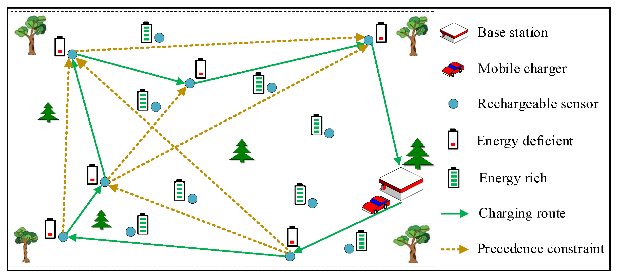
Motivated by the aforementioned issues, we propose the problem of scheduling wireless charging tasks with precedence constraints (SCPC), with the optimization objective of minimizing the completion time of all the charging tasks while guaranteeing that the energy capacity of the mobile charger (MC) is not exhausted, the deadline of each charging task is not exceeded, and no precedence constraints are violated. We give an instance of our problem, depicted in Figure 1, where there is one mobile charger (MC) and a set of rechargeable sensors located on a 2D plane. When the residual energy of a sensor falls below a certain threshold, it will send a charging request to the MC. In particular, there exist precedence constraints among the charging tasks raised by these sensors. The MC needs to visit all the energy-deficient sensors to fulfill the charging tasks without violating the precedence constraints. Thus, our objective is to design a optimal charging route to minimize the completion time when taking the precedence constraints among charging tasks into consideration.
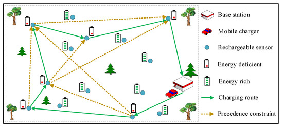
Figure 1.
A diagram of wireless charging tasks with precedence constraints.
For WRSNs, a great many existing works [13,14,15,16] focus on the mobile charging scenarios and aim to optimize the performance of the network, but none of them take the precedence relationships among charging tasks into consideration when studying charging issues. To the best of our knowledge, we are the first to propose charging issues with respect to the precedence relationships among tasks.
We face two main technical challenges when tackling this problem:
- The first challenge is to schedule the wireless charging tasks with precedence constraints by devising a closed path of travel for the MC which is NP-hard.
- The second challenge is that aside from the precedence constraints among charging tasks, more constraints need to be satisfied, including the deadline constraint of each charging task and the limited energy capacity constraint of the MC. These multiple constraints make our problem more complicated.
To address the first challenge, we propose a TS-based improved adaptive genetic algorithm to seek for the best solution (i.e., the individual with the best fitness value, derived through population evolution from one generation to the next iteratively). We first use a directed acyclic graph (DAG) to denote a set of charging tasks and complex precedence relationships among these tasks. As there are multiple feasible sequences that can be derived from one DAG, we propose a priority-based topological sorting scheme to obtain a unique feasible sequence on the DAG. Finally, we combine the priority-based topological sorting scheme with the procedure of a genetic algorithm to obtain the optimal sequence through selection, evaluation, and a series of genetic operators, including reproduction, crossover, and mutation. To address the second challenge, we design a fitness objective function by adding penalty weighting factors for deadline tardiness and extra consumed energy beyond the MC’s capacity to handle the multiple constraints in the SCPC problem. Specifically, we make the following main contributions:
- We are the first to propose the charging issues of scheduling an MC with respect to multiple constraints, including precedence constraints among charging tasks, the deadline constraint of the charging task, and the limited energy capacity constraint of the MC.
- We propose a TS-based improved adaptive genetic algorithm by combining the priority-based topological sorting scheme with the procedure of the improved adaptive genetic algorithm to find the best solution.
- We conduct extensive simulations to evaluate the performance of our proposed algorithm under the condition of three different network sizes. Our simulation results show that in terms of completion time, our proposed algorithm outperformed the other three comparison algorithms by up to .
The rest of the paper is organized as follows. Section 2 briefly surveys the related works. Section 3 illustrates the network model, task precedence relationship, and problem formulation. Section 4 demonstrates the proposed TS-based improved adaptive genetic algorithm for the SCPC problem in detail. Section 5 presents the results of the simulations. Finally, we conclude the paper in Section 6.
2. Related Work
Mobile charger optimization problem. There exists a great amount of research works [6,7,13,14,15,17,18] focusing on mobile charging scenarios where rechargeable devices are charged by one or multiple mobile chargers to maintain perpetual function. However, a great number of existing works do not take into consideration the energy issues regarding the task-level scheduling of a mobile charger. For example, Das et al. [6] focused on the joint data gathering and charging (DGAC) problem and introduced an efficient on-demand partial DGAC scheme using battery-limited multiple MVs to reduce the total dead periods of the sensors and the overall data gathering delay. Susan et al. [7] investigated the problem of scheduling a mobile charging vehicle (MCV) to wirelessly charge the rechargeable sensor nodes upon receiving a charging request and proposed a novel approach called scheduling on-demand charging requests with FFO-based optimal path (SOCR-FFO) selection, with the aim to jointly optimize the path selection for disseminating charging requests and scheduling MCVs based on the current network status. Shi et al. [13] introduced the concept of a renewable energy cycle in a sensor network and studied the optimization problem of maximizing the ratio of the wireless charging vehicle (WCV)’s vacation time over the cycle time. He et al. [14] investigated the on-demand mobile charging problem and employed a simple but efficient nearest job next with preemption (NJNP) discipline for a mobile charger. Liang et al. [15] studied sensor energy replenishment with a mobile charger in a rechargeable sensor network and aimed to maximize the sum of the charging rewards collected by all charged sensors from the mobile charger. Dudyala et al. [18] studied the problem of scheduling mobile chargers efficiently for charging the sensors so that the network would be up for the maximum time and proposed an efficient way of scheduling mobile chargers with the help of sensor energy consumption rate prediction.
Task scheduling problem in WRSNs. Some other works [16,19,20,21] considered charging task scheduling with or without task cooperation, but none of them took into account the precedence constraints among charging tasks. Wu et al. [16] explored the collaborated task-driven mobile charging and scheduling problem and aimed to maximize the overall task utility in the network by finding a closed charging tour with an energy allocation strategy. Dong et al. [19] explored the issue of maximizing the charger’s velocity to minimize the charging delay while guaranteeing that task assignment was feasible in WRSNs. Dai et al. [20] studied the problem of maximizing the overall effective charging energy for all rechargeable devices and further minimizing the total charging time through scheduling the power of wireless chargers while guaranteeing electromagnetic radiation (EMR) safety. In [21], Dai et al. further investigated the problem of charging task scheduling for directional wireless charger networks and maximized the overall charging utility for all tasks by scheduling the orientations of all chargers before a deadline in a centralized offline and distributed online fashion, respectively.
3. Problem Statement
3.1. Network Model
Suppose that there are some stationary rechargeable sensors located in a 2D plane which consume energy for sensing, data reception, and transmission. There is only one mobile charger (MC) with a limited energy capacity which is responsible for replenishing energy for all the sensors. Once the residual energy of a sensor falls below a certain threshold, it will launch the charging task and send the task to the MC. Within the sensor network, there is a fixed base station (BS), denoted by , which serves as a data sink as well as an energy source. An MC carrying a high-volume battery starts from the BS, tries its best to visit energy-deficient sensors, raising charging tasks for the energy supply, and returns to the BS after finishing the charging tour. Suppose that there are n charging tasks, denoted by . Formally, the ith charging task is defined by a four-tuple , where denotes the position of the rechargeable sensor that raises the task, is the release time of the task, is the deadline of the task, and is the required charging energy. We list the important notations in Abbreviations.
3.2. Task Precedence Relationship
Tasks often have precedence relationships between them, implying that a particular task can only be performed after another task has been completed. We write if task is an immediate successor of task or, equivalently, task is an immediate predecessor of task . This means that task raised by nodes cannot start before task raised by is completed, and thus the MC should visit node before node .
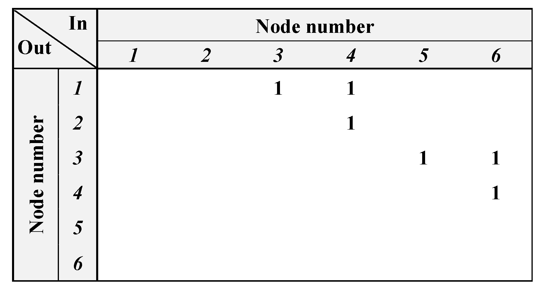
To represent the precedence relationships among tasks, we define the precedence matrix as
where indicates that task has to precede task .
An example of a precedence matrix is shown in Figure 2, containing six nodes with six precedence relationships. As shown in Figure 2, means that is an immediate predecessor of ; that is, node 1 should be visited before node 3. On the contrary, if , then there is no sequence relationship between and . Also, if rows 5 and 6 in the matrix have “” values, then this indicates that and have no successors. Similarly, columns 1 and 2 being blank means that and have no predecessors.
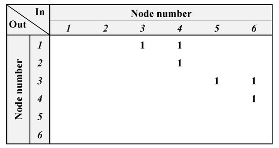
Figure 2.
An example of a precedence matrix. In the precedence matrix, there exist six precedence relationships among six nodes (No.1–No.6).
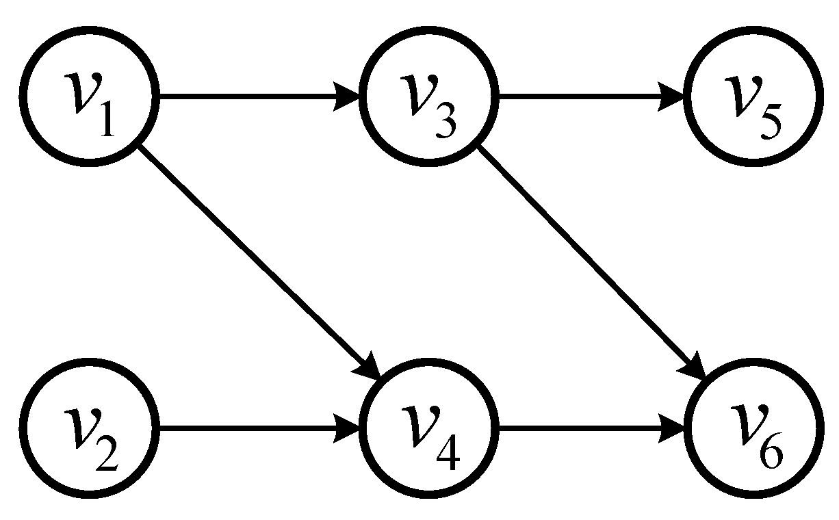
Using the precedence matrix in Figure 2, we can draw a directed graph, shown in Figure 3. Obviously, the directed graph must be acyclic; otherwise, no feasible solution exists. We can use a directed acyclic graph (DAG) to present a set of tasks and the precedence relationships among these tasks. An example of a DAG is shown in Figure 3, containing six nodes with six precedence relationships.
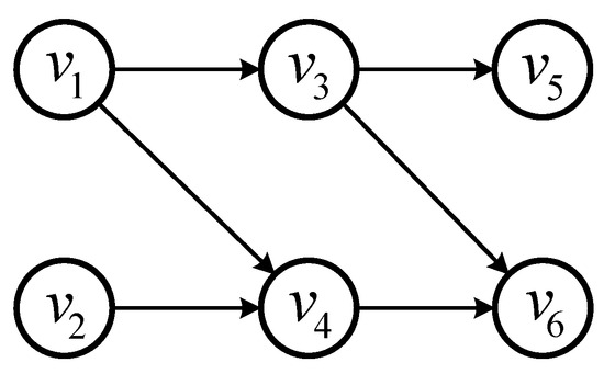
Figure 3.
An example of a DAG.
In the DAG, each vertex represents the charging task raised by node , and each arc indicates the precedence relationship .
3.3. Problem Formulation
We introduce a decision variable . The decision variable is one if and only if node precedes node immediately in a sequence; otherwise, it is zero.
The energy consumed by the MC when replenishing a WSN can be classified into two categories: the moving energy cost and charging energy cost. The moving energy cost of the MC is
where q is the energy consumption rate per unit length and is the distance between nodes and . In particular, and denote the distance between the BS and node . During wireless power transfer, energy loss is always inevitable, which depends on the charging distance and angle. Suppose that the MC consumes amount of energy when transferring one unit of energy to a node. Then, the charging energy cost for the nodes is
By combining the consumed energy for moving and charging during the closed charging sequence, the total energy cost of the MC can be expressed as
Let be the arrival time of the MC at node . As a task must be served at or after its release time and before its deadline, it can be derived that is between and . If the MC reaches a node before the release time, then it will bring about extra waiting time. We define the waiting time of the MC at node as , and thus . Note that should always be smaller than to prevent the nodes from running out of energy. The total completion time of finishing a tour, composed of the moving time, waiting time, and charging time, can be expressed as
where r is the traveling speed of the MC and is the energy receiving rate of the nodes.
Based on the aforementioned definitions and models, our objective is to minimize the completion time of all the charging tasks while guaranteeing that the energy capacity of the MC is not exhausted, the deadlines of the charging tasks are not exceeded, and no precedence constraints are violated. Therefore, we can formulate the scheduling wireless charging tasks with precedence constraints (SCPC) problem as
In the above formulation, Equations (6), (7), and (8) ensure the connectivity of the tour and that every node is visited only once. Equation (9) denotes the precedence relationship between nodes. Equation (10) guarantees the arrival time of the MC being within each task’s deadline. Equation (11) guarantees that the consumed energy will not exceed the MC’s capacity. Equation (12) restricts to be a value from 0 to 1. The SCPC problem can be reduced to the traveling salesman problem with precedence constraints (TSPPC), with the MC’s energy capacity being unlimited and the unspecified task’s deadline being unlimited. Clearly, since the TSPPC belongs to the scope of NP-hard problems [22], the SCPC problem is also NP-hard.
4. TS-Based Improved Adaptive Genetic Algorithm
In this section, we propose a TS-based improved adaptive genetic algorithm to tackle the thorny SCPC problem. The genetic algorithm (GA) is one of the evolutionary search methods that attempts to find a good (or best) solution for specific problems, such as combinatorial optimization problems. The basic principles of the GA were first proposed by Holland in 1975 [23]. Genetic programming is based on the Darwinian principle of reproduction (i.e., survival of the fittest). The utilization of a genetic algorithm is finding the individual with the best fitness value from the search space of the problem.
Because precedence constraints exist in the SCPC problem, the traditional representation schemes in a GA algorithm generate infeasible solutions, which would conflict with the precedence constraints. To handle this conflict, we propose a TS-based improved adaptive genetic algorithm.
4.1. Priority-Based Topological Sorting Scheme
In the aforementioned directed acyclic graph (DAG), the vertices denote charging tasks raised by the nodes, and the edges represent the precedence relationships among the tasks. A solution to the SCPC problem must involve a linear ordering of the nodes satisfying all the precedence constraints of the edges on a DAG.
Several definitions related to topological sorting need to be introduced before investigating the process of topological sorting.
Definition 1.
One topological sorting (also called topological ordering) of a DAG is a linear ordering of all its vertices such that for every directed edge from vertex u to vertex v, vertex u comes before vertex v in the ordering [24].
Definition 2.
The indegree of one vertex is the number of edges which terminate into the vertex [25].
The process of topological sorting involves searching for a feasible linear ordering of the vertices on a DAG. One DAG may have multiple feasible sequences. In order to decide upon a unique sequence among all feasible ones, a priority assignment scheme is used; that is, a different priority value is assigned to each vertex on the graph randomly. The priority of each vertex is generated within randomly and exclusively, where n is the number of vertices or tasks. The only feasible sequence can be derived from one priority string by combining the priority assignment scheme with topological sorting (i.e., the proposed priority-based topological sorting scheme), and thus one priority string can represent a unique, feasible sequence.
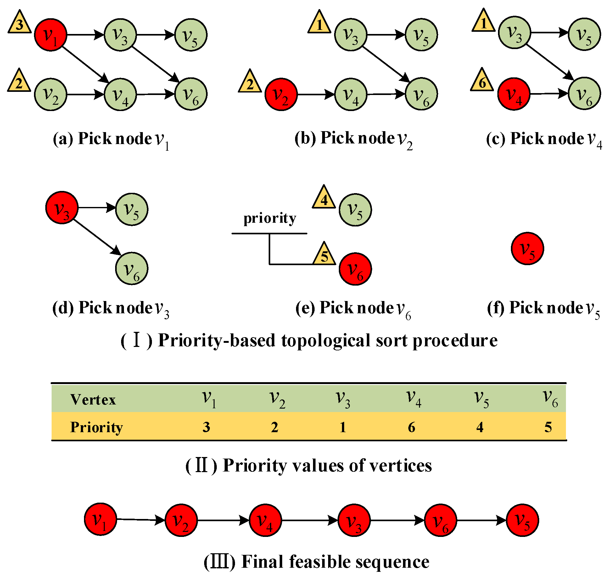
Algorithm 1 presents the pseudo-code for the priority-based topological sorting scheme on a DAG. Figure 4 shows an instance of generating a feasible sequence using the priority-based topological sorting scheme. Figure 4(I) demonstrates the process of topological sorting with the assigned priority that is shown in Figure 4(II), and the final feasible path is displayed in Figure 4(III). In the initial graph in Figure 4(I)(a), the indegree values of vertices and are equal to zero. Vertex was selected as the first point because its priority, which is was three as marked in the yellow triangle, was higher than the priority of vertex (two), and vertex was stored in the queue. Then, for vertex , its outgoing edges and were removed from the graph. In the generation graph in Figure 4(I)(b), vertex was picked in the same manner, and then vertex and its outgoing edges were also removed from the graph. As shown in Figure 4(I)(c–f), we continued this procedure until all the vertices were visited, and then a final sequence was uniquely derived for the priority string “321645”. The solution path is represented by the priority string “321645”.
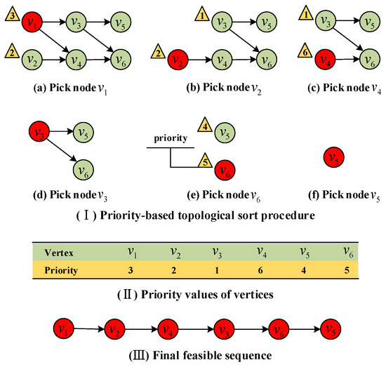
Figure 4.
An example of a priority-based topological sorting scheme.
Each individual of the population is represented as a string of integers, and each digit of the string indicates the priority of the vertex and ranges between one and the number of vertices. The initialization of the population of chromosomes (i.e., a series of integer strings) is generated randomly, and the population size is predetermined.
| Algorithm 1 Priority-based topological sorting scheme. |
| INPUT Directed acyclic graph OUTPUT Feasible sequence on the directed acyclic graph Initialization Phase
|
4.2. Objective and Fitness Value
To evaluate the goodness of each individual, the fitness value of each individual should be measured with the proper objective function. The objective of the SCPC problem is to minimize the completion time of serving a set of charging tasks without violating the precedence constraints, missing the deadlines of tasks, or exceeding the battery capacity of the MC. The individuals represented by the randomly assigned priority strings will satisfy the precedence constraints in Equation (9) according to the above analysis. However, it cannot ensure that these individuals meet the deadlines of the tasks in Equation (10) or the capacity constraint of the MC in Equation (11). Considering the complex constraints in the SCPC problem, we adopted the penalty function method from [26] to construct a new criterion for measuring the fitness, which we call the modified objective function:
The modified objective function includes terms weighted by coefficients for the touring time, for the waiting time at the nodes, and penalty weighting factors for tardiness of task deadlines and for extra consumption energy beyond the MC’s capacity. Specifically, the charging time item is removed from the objective function, since the charging time is constant for different individuals. It is critical to assign proper values to these coefficients of the objective function. We gave lower weights to coefficients and and much higher weights to penalty factors and . For example, we can set , , , and . The set of weights is biased toward searching for feasible solutions in comparison with reducing the total completion time. If there is no violation of the tasks’ deadlines and the MC’s capacity constraints, then the function is to reduce the total completion time. The weights of the coefficients of the objective function are chosen to prioritize exploring for feasible solutions and then minimize the total completion time under the precondition of the feasibility of solutions.
4.3. Selection Mechanisms
The selection operator is concerned with improving the average quality of the population by giving high-quality chromosomes a better chance for further reproduction. We employed the two most popular selection operators: the roulette wheel selection mechanism and elitist strategy.
In the roulette wheel selection mechanism, the probability of one chromosome being selected for survival into the further evolution process is closely related to its fitness value. The selected probability of one individual is higher with a better fitness value. This means that the average quality of the population is improving by giving the high-quality chromosomes a better chance to be reproduced into the next generation. Moreover, the elitist strategy is employed to ensure that one or a number of the best chromosomes can be copied into the next generation.
4.4. Genetic Operators
Generally, a GA is composed of three operators: reproduction, crossover, and mutation. By using the three operators, one generation is evolved into the next generation iteratively. Some of the best individuals are reproduced from the current generation into the next generation using the elitist strategy.
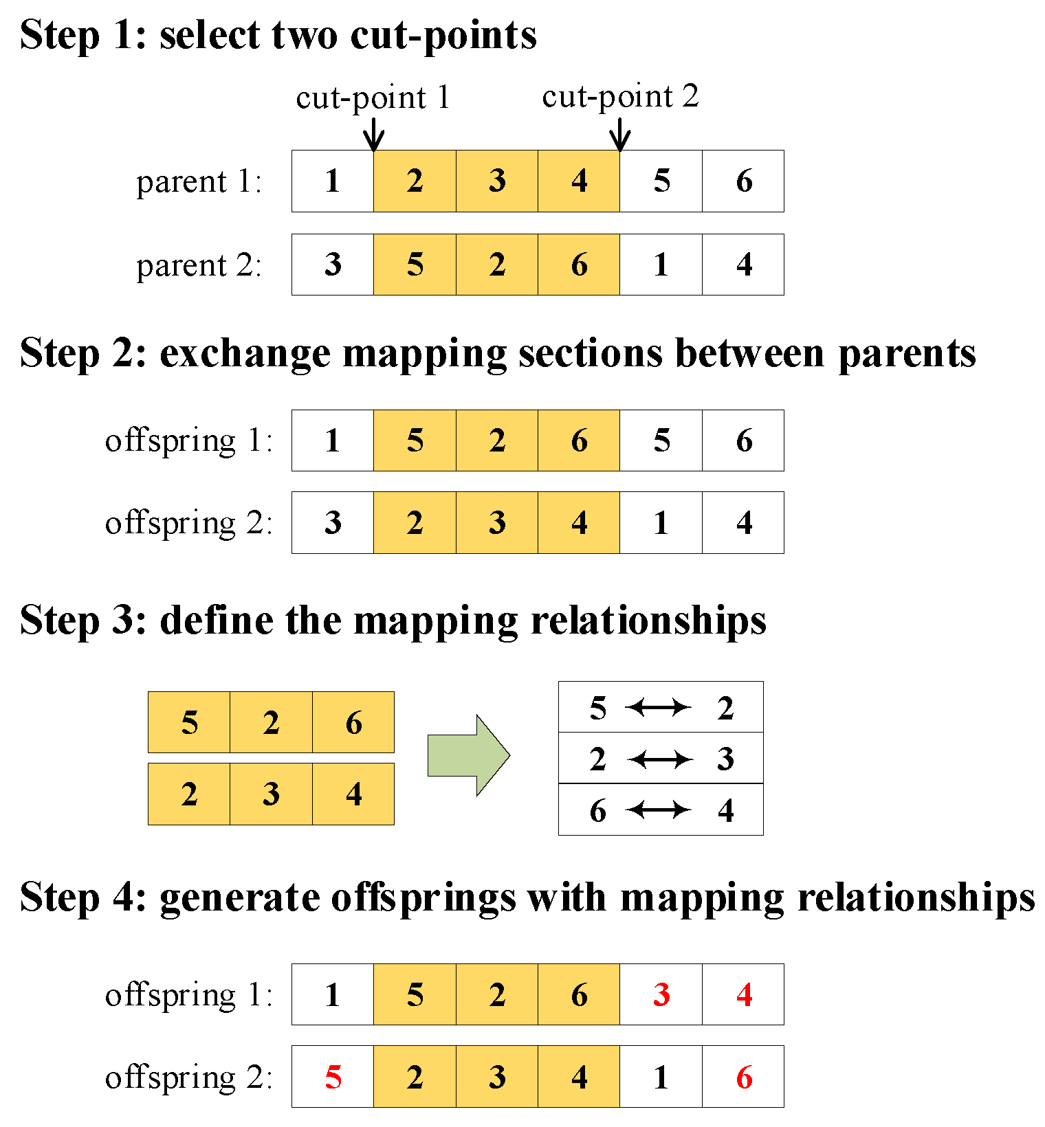
The crossover operation is the main evolutionary operator, and it works by recombining genes from different parents to generate a new one, called the offspring. Once the parents have been selected with the roulette wheel selection mechanism, the crossover operator is applied according to the crossover probability. Through the crossover operation, many excellent new individuals are continuously generated to expand the search range of the algorithm in the entire space and ensure the excellent search performance of the genetic algorithm. There are many crossover operators proposed in the literature for genetic operators. One of the most-used crossover operators is the partially mapped crossover (PMX) operator adapted to the path planning case. The PMX operator was suggested by Goldberg and Lingle [27]. Figure 5 illustrates an example including the four steps of the PMX operator. In Step 1, it randomly selects two cut points along the two parents strings uniformly. Suppose that the first cut point is selected between the first and second string elements, and the second one is between the fourth and fifth string elements. The substrings between the two cut points are known as mapping sections. In Step 2, the selected mapping sections are exchanged between parents; that is, the mapping section “234” of the first parent is copied into the second offspring. Correspondingly, the mapping section “526” of the second parent is copied into the first offspring. Then, the first offspring is filled up by copying the remaining elements of the first parent, as is the second offspring. In Step 3, the mapping relationships are defined according to the mapping sections (i.e., , , and ). The digits in one chromosome, denoting the priorities of the vertices, are different from each other. In Step 4, in case a digit is already present in the offspring, it is replaced according to the mapping relationships. For example, the fifth element of the first offspring would be digit 5, which is already present in the mapping section. Hence, digit 5 is replaced by digit 3 according to the mappings and . Analogously, the sixth element of the first offspring and the first and sixth elements of the second offspring are updated to digit 4, digit 5, and digit 6, respectively.
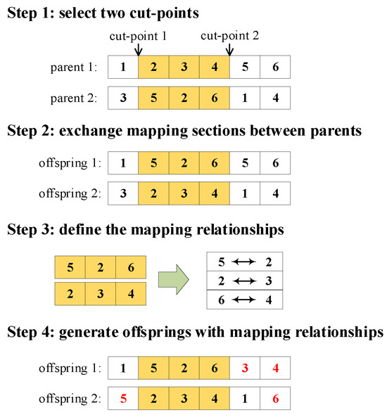
Figure 5.
Illustration of the PMX.
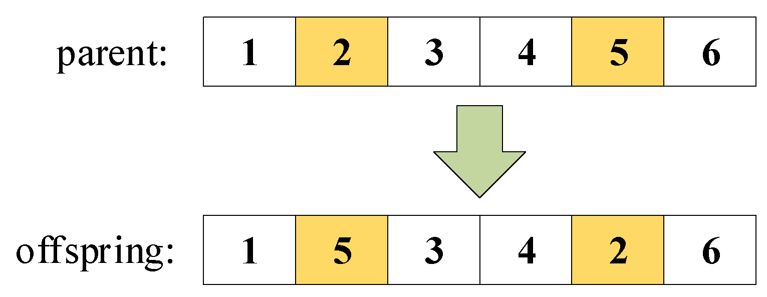
The mutation operator and crossover operator play different roles in a genetic algorithm. Mutation operations are usually used in conjunction with crossover operations to improve the global search performance of algorithms. When the algorithm is approaching the optimal solution, appropriate mutation operations can effectively accelerate the convergence speed of the algorithm. A mutation operation is applied to explore new states by making a change in one chromosome, thus preventing premature convergence to a dominant result by introducing diversification into the population. The exchange mutation (EM) [28] is employed in our algorithm. The EM randomly selects two genes within a chromosome and exchanges them. As shown in Figure 6, one chromosome is represented by string “123456”, and suppose that the second and fifth genes are randomly selected. This results in new chromosome represented by string “153426” by employing the EM operator.
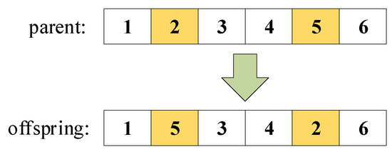
Figure 6.
Illustration of the EM.
4.5. Adaptive Crossover Probability and Mutation Probability
The selections of the crossover probability and mutation probability play a critical role in the performance of genetic algorithms. Scientific and reasonable probability parameters can effectively avoid premature convergence of the local optimal solution and improve the global search performance of genetic algorithms. In traditional genetic algorithms, the crossover probability and mutation probability are empirical values and are often fixed and invariant. In order to better screen out outstanding individuals and improve the search efficiency of global optimal solutions, the genetic algorithm will be optimized by adjusting the crossover and mutation probabilities dynamically. The fitness values of individuals in the population are used as important reference indicators for the crossover and mutation probabilities.
The crossover operation is the most core part of a genetic algorithm, taking responsibility for individual gene recombination. As the only indicator of the strength of crossover operations, the selection of crossover probability values is crucial. If the crossover probability value is too large, then although the search space of the algorithm will increase, the overall efficiency of the algorithm will be affected. If the crossover probability value is too small, then the algorithm is highly likely to become slow and inefficient, greatly reducing global search performance. Repeated experiments are required to determine the crossover probability for different optimization problems, making it difficult to find the optimal crossover probability suitable for each problem. M. Srinivas et al. proposed an adaptive genetic algorithm [29] in which the crossover probability is continuously adjusted according to the fitness values of individuals. In the adaptive genetic algorithm [29], the crossover probability approaches or equals zero when the fitness of an individual is close to or equal to the maximum fitness of the population. This is unfavorable for the early stage of evolution, as the excellent individuals at the early stage remain almost unchanged, increasing the likelihood of evolution toward a local optimal solution. In order to overcome this problem, an improved adaptive crossover probability is proposed. For individuals with the highest or lowest fitness, no crossover operation or complete crossover operation has been avoided. Instead, the crossover operation is carried out with a specific probability. It effectively enhances the role of the crossover operation in maintaining individual diversity in the algorithm. The adjusted crossover probability is
where is the crossover probability, and are certain constants, f is the larger fitness value between two parents for the crossover operation, and and are the maximum and minimum fitness values in the population, respectively.
The mutation operation is also an indispensable part of genetic algorithms, ensuring the diversity of individuals in the population. In mutation operations, the intensity of mutation operations is represented by the mutation probability. The value of the mutation probability has a significant impact on the entire algorithm. The mutation probability is usually small, which can prevent the loss of excellent genes in the population. If the value is too large, then the algorithm will become a pure random search algorithm and lose its original characteristics. Similarly, the mutation probability in [29] had the issue of the mutation probability for individuals with the highest fitness being equal to zero. In the same way, the adaptive mutation probability is optimized as follows:
where is the mutation probability, and are certain constants, and f is the fitness value of an individual for the mutation operation.
Algorithm 2 demonstrates the detailed process of our proposed TS-based improved adaptive genetic algorithm. In the working phase, a DAG is derived from the given precedence constraints (Step 1), and then individuals represented by the chromosomes in the current population are deduced by employing Algorithm 1 (Step 3). After that, the fitness values of individuals are estimated (Step 4), and the elitist strategy and roulette wheel selection mechanism are performed (Step 5 and 6). Finally, the selected parents from the current population are evolved into offspring for the next generation by using genetic operators (i.e., reproduction, crossover, and mutation) (Steps 7–9).
| Algorithm 2 TS-based improved adaptive genetic algorithm. |
| INPUT Precedence constraints; GA parameters OUTPUT Best chromosome Initialization Phase
|
5. Simulation Results
In this section, we conduct extensive simulation experiments to demonstrate the performance of our proposed TS-based improved adaptive genetic algorithm (TS-IAGA) in terms of its effectiveness and efficiency.
5.1. Evaluation and Baseline Set-Up
We utilized the following parameter set-up in the simulation unless otherwise stated. We supposed that charging tasks were uniformly distributed in a 20 m × 20 m square area, and the energy requirement of the charging tasks ranged from 5 J to 10 J. We set (task number 6), (task number 20), or (task number 50) and , , , , , , , , , , , and . Aside from that, the release time and deadline of the charging task were generated in the range of and , respectively. We introduced three charging schemes for comparison: the TS-based genetic algorithm (TS-GA) [30], earliest deadline first policy (EDF) [31], and nearest job next with preemption discipline (NJNP) [14]. For the TS-GA, the crossover probability in the gene algorithm is an invariant constant and fixed throughout the entire crossover operation process, and the same applies for the mutation probability, which is also constant during the mutation operation. For the EDF, the MC always serves the node with the earliest deadline. For the NJNP, the nearest node will be served first by the MC. Moreover, each data point in the following figures stands for an average result for 100 topologies generated randomly.
5.2. Performance Comparison
In the following subsections, we compare our TS-IAGA with the TS-GA, EDF, and NJNP in terms of the total completion time considering problems with three different complexity degrees (i.e., networks containing 6 tasks, 20 tasks, and 50 tasks).
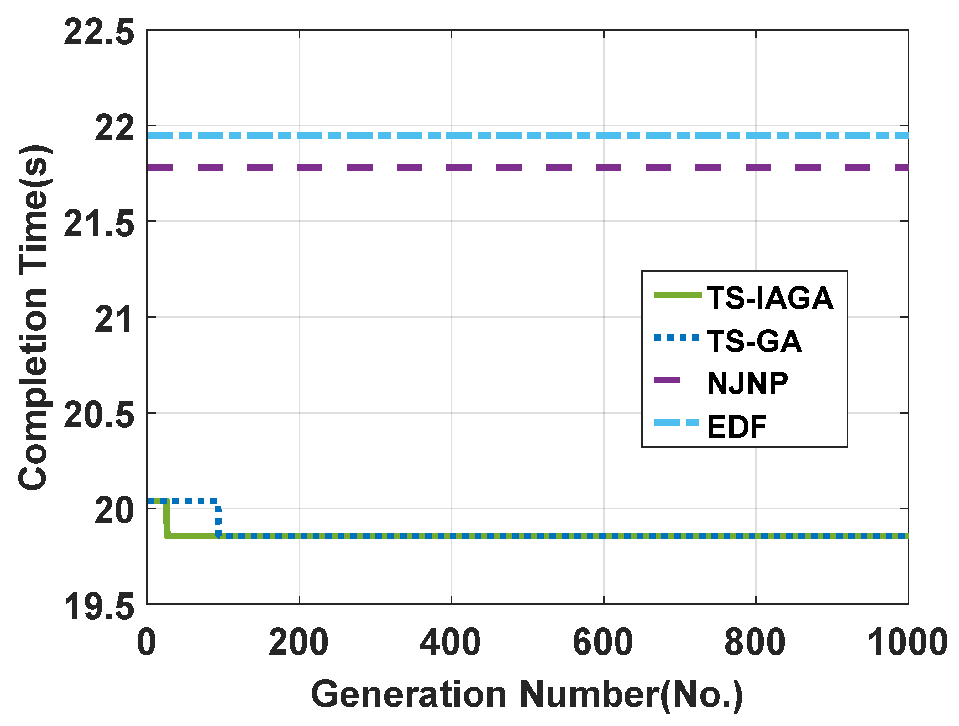
5.2.1. Completion Times for Six Tasks
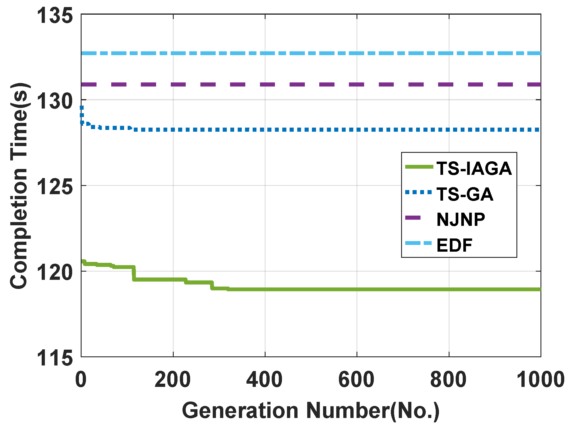
Our algorithm outperformed the EDF and NJNP by up to and , respectively, as the generation number increased from 0 to 1000 when there were 6 tasks in the network. In additon, although the final solution of our algorithm was equal to that of the comparison TS-GA, our algorithm converged to the final solution earlier than the TS-GA. The simple network topology was composed of six vertices and six precedence constraints. In Figure 7, the completion time of the EDF and NJNP remained constant since the parameter generation number was unrelated to both the EDF and NJNP. In addition, the completion time of the TS-IAGA dropped off as the generation number increased. Furthermore, the TS-IAGA converged to the final solution at generation number 26, while the TS-GA converged after generation number 94. Obviously, the TS-IAGA had a greater search efficiency than the TS-GA.
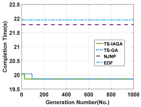
Figure 7.
Completion time vs. generation number (task number 6).
5.2.2. Completion Time for Twenty Tasks
Our algorithm outperformed the TS-GA, EDF, and NJNP by , , and , respectively, as the generation number increases from 0 to 1000 when there were 20 tasks in the network. The more complex network topology was composed of 20 vertices and 21 precedence constraints. The variation tendency of the completion time for the four algorithms is illustrated in Figure 8. As usual, we can see that the completion time of the EDF and NJNP did not change with varying generations. A little different from Figure 7, the completion time for the TS-IAGA tended to decrease relatively stably as the generation number increased. Additionally, the TS-IAGA converged to the final solution at a later generation (285) in comparison with when there was simply six tasks.
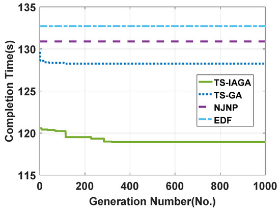
Figure 8.
Completion time vs. generation number (task number 20).
5.2.3. Completion Time for Fifty Tasks
Our algorithm outperformed the TS-GA, EDF, and NJNP by , , and , respectively, as the generation number increased from 0 to 1000 when there were 50 tasks in the network. For a larger problem, we considered a network topology with 50 vertices and 68 precedence constraints. As depicted in Figure 9, the completion time of the EDF and NJNP still remained unchanged regardless of the variation in the generation number. Aside from that, the trend of the completion time for the TS-IAGA declined at a lower pace when the generation number increased. Moreover, the TS-IAGA converged to the final solution at an even later generation (617) compared with the previous results in Figure 7 and Figure 8.
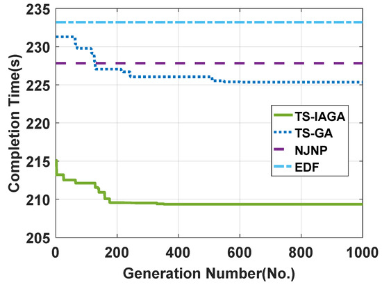
Figure 9.
Completion time vs. generation number (task number 50).
5.3. Insights
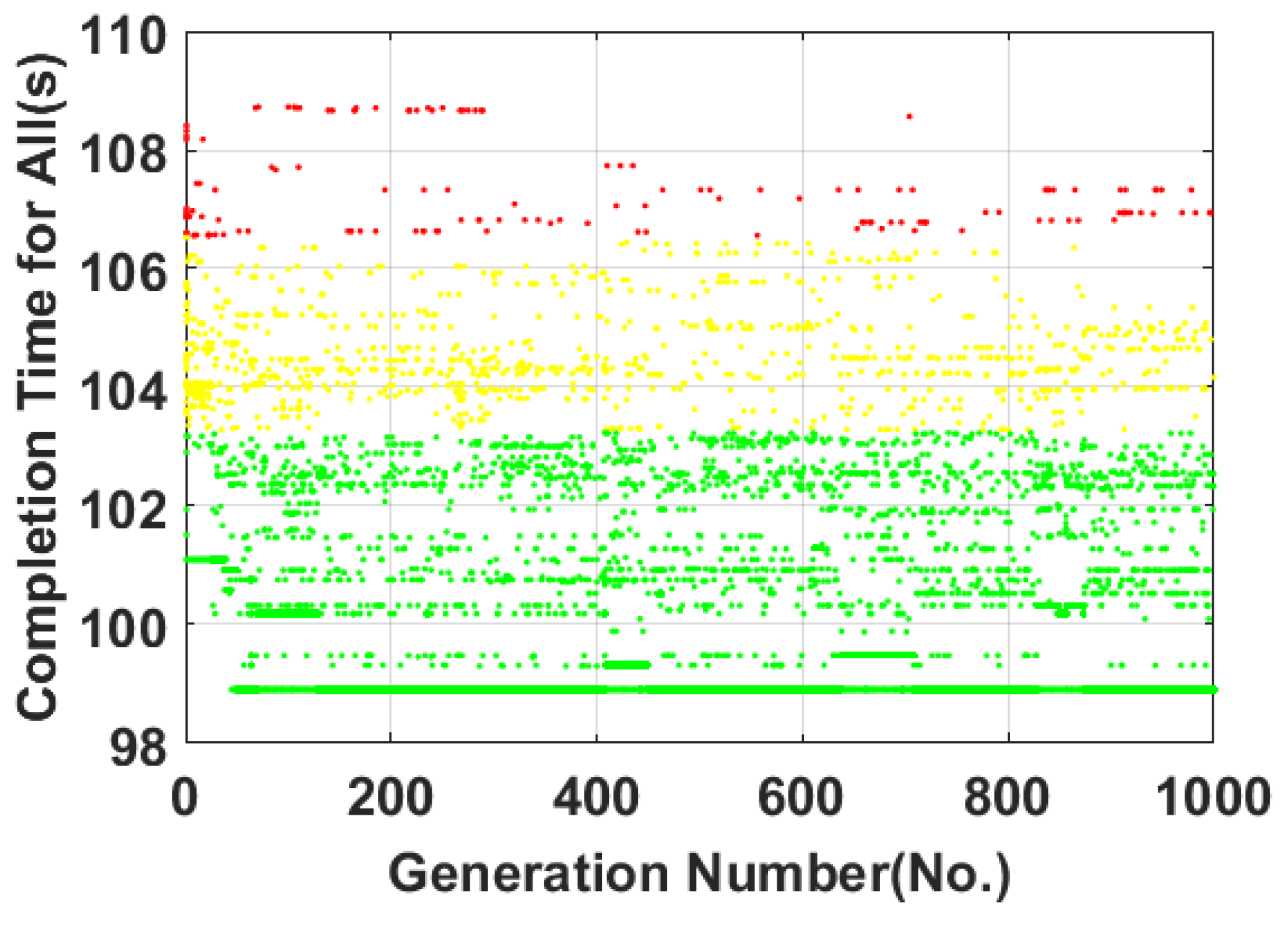
In this subsection, we depict the distribution of the completion times of each individual in every generation to indicate the performance of our proposed algorithm. In Figure 10, the red dots denote the poor output results of the TS-IAGA, and yellow dots signify mediocre output results, while green dots indicate relatively better output results. We set two constant threshold values, and , which were between the minimum and maximum completion times, and was less than . When the completion time of one individual at a certain generation was less than , the corresponding dot was colored green, and when the result of one individual was between and , the corresponding dot was painted yellow, while a red dot signifies that the completion time of the corresponding individual was larger than . It can be observed that the quantity of red dots became lower and lower and the number of yellow dots did not vary too much, merely becoming slightly lower. With regard to the amount of green dots, it increased, which further validates the effectiveness of our proposed algorithm.

Figure 10.
Completion times for all individuals vs. generation number (task number 20). Note: The overall distribution map of population individuals presents the completion times of 50 individuals at each generation when there were 20 tasks in the network and was set to 50. One dot indicates the completion time of one individual at a certain generation. Moreover, red dots denote relatively poor results, and yellow dots signify mediocre results, while green dots indicate relatively better results.
6. Conclusions
The key novelty of this paper is that we are the first to raise the issue of scheduling of wireless charging tasks with precedence constraints in wireless rechargeable sensor networks. The key contribution of this paper is proposing a TS-based improved adaptive genetic algorithm and conducting simulations for evaluation under networks of three different complexity degrees. In order to obtain a unique, feasible sequence satisfying the precedence constraints in the SCPC problem, we proposed a priority-based topological sorting scheme. By combining the priority-based topological sorting scheme with the procedure of an improved adaptive genetic algorithm, we searched for the optimal sequence iteratively. Moreover, we constructed the modified fitness objective function by adding penalty terms to tackle the additional constraints. Our evaluation results show that in terms of completion time, our proposed algorithm outperformed the three comparison algorithms by up to .
Author Contributions
Conceptualization and methodology, L.L.; formal analysis, L.L.; resources and supervision, H.D.; software and validation, C.C. and S.L.; writing—original draft preparation, L.L.; writing—review and editing, H.D. and Z.N. All authors have read and agreed to the published version of the manuscript.
Funding
This work was partially supported by the Future Network Scientific Research Fund Project FNSRFP-2021-YB-52 and 2022 Nanhang Jincheng College Scientific Research Fund Project under grant number XJ202204.
Data Availability Statement
Data is contained within the article.
Conflicts of Interest
The authors declare no conflicts of interest.
Abbreviations
The following abbreviations are used in this manuscript:
| Symbol | Meaning |
| MC | Mobile charger |
| BS | Base station |
| Sensor (node) i | |
| , T | The ith charging task, task set |
| n | Number of charging tasks |
| Required charging energy of charging task | |
| Release time of charging task | |
| Deadline of charging task | |
| Waiting time of MC at node | |
| Distance between nodes and | |
| r | Traveling speed of MC |
| Battery capacity of MC | |
| Energy receiving rate of node | |
| q | Energy consumption rate of MC per unit length |
| Energy consumption of MC for transferring one unit of energy to node | |
| Arrival time of MC at node | |
| Adaptive crossover probability | |
| Adaptive mutation probability | |
| Population size | |
| Number of generation |
References
- Zhang, J.; Gao, H.; Chen, Q.; Li, J. Task-oriented energy scheduling in wireless rechargeable sensor networks. ACM Trans. Sens. Netw. 2023, 19, 88. [Google Scholar] [CrossRef]
- He, S.; Chen, J.; Jiang, F.; Yau, D.K.; Xing, G.; Sun, Y. Energy provisioning in wireless rechargeable sensor networks. IEEE Trans. Mob. Comput. 2012, 12, 1931–1942. [Google Scholar] [CrossRef]
- Yildirim, K.S.; Carli, R.; Schenato, L. Safe distributed control of wireless power transfer networks. IEEE Internet Things J. 2019, 6, 1267–1275. [Google Scholar] [CrossRef]
- Ding, X.; Wang, Y.; Sun, G.; Luo, C.; Li, D.; Chen, W.; Hu, Q. Optimal charger placement for wireless power transfer. Comput. Netw. 2020, 170, 107123. [Google Scholar] [CrossRef]
- Gao, W.; Li, Y.; Shao, T.; Lin, F. An On-Demand partial charging algorithm without explicit charging request for WRSNs. Electronics 2023, 12, 4343. [Google Scholar] [CrossRef]
- Das, R.; Dash, D. Joint on-demand data gathering and recharging by multiple mobile vehicles in delay sensitive WRSN using variable length GA. Comput. Commun. 2023, 204, 130–146. [Google Scholar] [CrossRef]
- Susan, T.S.A.; Balasubramanian, N. Scheduling on-demand charging request in wireless rechargeable sensor network with fruit fly optimization-based path selection. Int. J. Inf. Technol. 2022, 14, 2377–2388. [Google Scholar] [CrossRef]
- Singh, J.; Sajid, M.; Yadav, C.S. An efficient approach for wireless rechargeable sensor networks for vehicle charging. In Proceedings of the International Conference on Augmented Intelligence and Sustainable Systems (ICAISS), Trichy, India, 24–26 November 2022. [Google Scholar]
- Kaswan, A.; Jana, P.K.; Das, S.K. A survey on mobile charging techniques in wireless rechargeable sensor networks. IEEE Commun. Surv. Tutor. 2022, 24, 1750–1779. [Google Scholar] [CrossRef]
- Dai, H.; Ma, Q.; Wu, X.; Chen, G.; Yau, D.K.Y.; Tang, S.; Li, X.-Y.; Tian, C. CHASE: Charging and scheduling scheme for stochastic event capture in wireless rechargeable sensor networks. IEEE Trans. Mob. Comput. 2018, 19, 44–59. [Google Scholar] [CrossRef]
- Guo, S.; Wang, C.; Yang, Y. Joint mobile data gathering and energy provisioning in wireless rechargeable sensor networks. IEEE Trans. Mob. Comput. 2014, 13, 2836–2852. [Google Scholar] [CrossRef]
- Sparks, P. The Route to a Trillion Devices. Available online: https://community.arm.com/iot/b/blog/posts/whitepaper-the-route-to-a-trillion-devices (accessed on 12 July 2017).
- Shi, Y.; Xie, L.; Hou, Y.T.; Sherali, H.D. On renewable sensor networks with wireless energy transfer. In Proceedings of the IEEE INFOCOM, Shanghai, China, 10–15 April 2011; pp. 1350–1358. [Google Scholar]
- He, L.; Kong, L.; Gu, Y.; Pan, J.; Zhu, T. Evaluating the on-demand mobile charging in wireless sensor networks. IEEE Trans. Mob. Comput. 2015, 14, 1861–1875. [Google Scholar] [CrossRef]
- Liang, W.; Xu, Z.; Xu, W.; Shi, J.; Mao, G.; Das, S.K. Approximation algorithms for charging reward maximization in rechargeable sensor networks via a mobile charger. IEEE/ACM Trans. Netw. 2017, 35, 3161–3174. [Google Scholar] [CrossRef]
- Wu, T.; Yang, P.; Dai, H.; Xu, W.; Xu, M. Collaborated tasks-driven mobile charging and scheduling: A near optimal result. In Proceedings of the IEEE INFOCOM, Paris, France, 29 April–2 May 2019. [Google Scholar]
- Wang, Y.; Su, Z.; Zhang, N.; Li, R. Mobile wireless rechargeable UAV networks: Challenges and solutions. IEEE Commun. Mag. 2022, 60, 33–39. [Google Scholar] [CrossRef]
- Dudyala, A.K.; Ram, L.K. Improving the lifetime of wireless rechargeable sensors Using mobile charger in On-Demand charging environment based on energy consumption rate prediction. In Proceedings of the International Conference on Computational Electronics for Wireless Communications, Surathkal, India, 9–10 June 2022. [Google Scholar]
- Dong, Z.; Liu, C.; Fu, L.; Cheng, P.; He, L.; Gu, Y.; Gao, W.; Yuen, C.; He, T. Energy synchronized task assignment in rechargeable sensor networks. In Proceedings of the IEEE SECON, London, UK, 27–30 June 2016; pp. 1–9. [Google Scholar]
- Dai, H.; Ma, H.; Liu, A.X.; Chen, G. Radiation constrained scheduling of wireless charging tasks. In Proceedings of the ACM MobiHoc, Chennai, India, 10–14 July 2017. [Google Scholar]
- Dai, H.; Sun, K.; Liu, A.X.; Zhang, L.; Zheng, J.; Chen, G. Charging task scheduling for directional wireless charger networks. In Proceedings of the ICPP, Eugene, OR, USA, 13–16 August 2018. [Google Scholar]
- Moon, C.; Kim, J.; Choi, G.; Seo, Y. An efficient genetic algorithm for the traveling salesman problem with precedence constraints. Eur. J. Oper. Res. 2002, 140, 606–617. [Google Scholar] [CrossRef]
- Holland, J.H. Adaptation in Natural and Artificial Systems; The University of Michigan Press: Ann Arbor, MI, USA, 1975. [Google Scholar]
- Ajwani, D.; Friedrich, T. Average-case analysis of incremental topological ordering. Discret. Appl. Math. 2010, 158, 240–250. [Google Scholar] [CrossRef]
- Ma, J.; Iwama, K.; Takaoka, T.; Gu, Q.P. Efficient parallel and distributed topological sort algorithms. In Proceedings of the IEEE International Symposium 518 on Parallel Algorithms Architecture Synthesis, Aizu-Wakamatsu, Japan, 17–21 March 1997. [Google Scholar]
- Schoenauer, M.; Xanthakis, S. Constrained GA optimization. In Proceedings of the 5th International Conference on Genetic Algorithms, Champaign, IL, USA, 17–21 July 1993. [Google Scholar]
- Goldberg, D.E.; Robert Lingle, J. Alleles, Loci and the Traveling saleman problem. In Proceedings of the First International Conference on Genetic Algorithms and Their Applications, Pittsburg, PA, USA, 24–26 July 1985. [Google Scholar]
- Banzhaf, W. The molecular traveling salesman. Biol. Cybern. 1990, 64, 7–14. [Google Scholar] [CrossRef]
- Srinivas, M.; Patnaik, L. Adaptive probabilities of crossover and mutation in genetic algorithms. IEEE Trans. Syst. Man Cybern. 1994, 24, 656–667. [Google Scholar] [CrossRef]
- Li, L.; Yue, L.; Dai, H.; Yu, N.; Chen, G. Scheduling of wireless charging tasks with precedence constraints. In Proceedings of the IEEE Symposium on Computers and Communications (ISCC), Rennes, France, 7–10 July 2020. [Google Scholar]
- Stankovic, J.A.; Spuri, M.; Ramamritham, K.; Buttazzo, G. Deadline Scheduling for Real-Time Systems: EDF and Related Algorithms; Springer Science & Business Media: Berlin/Heidelberg, Germany, 2012; Volume 460. [Google Scholar]

Disclaimer/Publisher’s Note: The statements, opinions and data contained in all publications are solely those of the individual author(s) and contributor(s) and not of MDPI and/or the editor(s). MDPI and/or the editor(s) disclaim responsibility for any injury to people or property resulting from any ideas, methods, instructions or products referred to in the content. |
© 2024 by the authors. Licensee MDPI, Basel, Switzerland. This article is an open access article distributed under the terms and conditions of the Creative Commons Attribution (CC BY) license (https://creativecommons.org/licenses/by/4.0/).