Accelerating Strawberry Ripeness Classification Using a Convolution-Based Feature Extractor along with an Edge AI Processor

Abstract

Image analysis-based artificial intelligence (AI) models leveraging convolutional neural networks (CNN) take a significant role in evaluating the ripeness of strawberry, contributing to the maximization of productivity. However, the convolution, which constitutes the majority of the CNN models, imposes significant computational burdens. Additionally, the dense operations in the fully connected (FC) layer necessitate a vast number of parameters and entail extensive external memory access. Therefore, reducing the computational burden of convolution operations and alleviating memory overhead is essential in embedded environment. In this paper, we propose a strawberry ripeness classification system utilizing a convolution-based feature extractor (CoFEx) for accelerating convolution operations and an edge AI processor, Intellino, for replacing FC layer operations. We accelerated feature map extraction utilizing the CoFEx constructed with systolic array (SA) and alleviated the computational burden and memory overhead associated with the FC layer operations by replacing them with the k-nearest neighbors (k-NN) algorithm. The CoFEx and the Intellino both were designed with Verilog HDL and implemented on a field-programmable gate array (FPGA). The proposed system achieved a high precision of 93.4%, recall of 93.3%, and F1 score of 0.933. Therefore, we demonstrated a feasibility of the strawberry ripeness classification system operating in an embedded environment.

1. Introduction

Recently, AI technologies have undergone rapid development, bringing significant changes to the field of agriculture. Research and applications utilizing AI to enhance agricultural productivity and promote sustainable farming practices have emerged diversely [1,2,3]. Within the domain of AI applications, image analysis models assume a critical role in shaping agricultural production and management. Image-based AI models contribute significantly to discerning the state of crops and evaluating the ripeness of fruits, thereby predicting the optimal harvesting time to maximize productivity [4,5,6]. Particularly, accurately measuring the ripeness of fruits in this field is emphasized as a key task in the modern agricultural paradigm to optimize yield and resource utilization. Strawberries, being a representative crop, enable the evaluation of ripeness levels based on color. Strawberries are economically valuable fruits due to their sweet taste and rich nutritional content [7,8]. The flavor and market impact of strawberries are significantly influenced by their degree of ripeness. A more advanced level of ripening results in distinct taste variations and has considerable implications for distribution. For these reasons, evaluating the appropriate ripeness of strawberries is essential as it enhances the marketability and economic viability of the fruit through timely harvesting [9].

To harvest strawberries at the right time, the characteristics of strawberries must be accurately extracted and classified according to their ripeness. Specifically, finding unique patterns or structures within images is crucial for extracting appropriate features from the images. Traditional methods for feature extraction include algorithms such as scale-invariant feature transform (SIFT), speeded-up robust features (SURF), and features from accelerated segment test (FAST). SIFT is an algorithm that detects features in an image that are invariant to scale and rotation [10]. SURF improves upon SIFT, providing faster processing speeds [11]. FAST is a computer vision algorithm that rapidly detects corners in an image, identifying keypoints based on intensity differences between central and neighboring pixels [12]. However, deep learning (DL), which automatically learns features from large amounts of data and is applicable to various complex tasks, has demonstrated higher performance and versatility compared to traditional feature extraction methods.

Among DL models for image analysis, CNN models especially demonstrate excellent performance in extracting features and learning from images, making them effective in analyzing images in complex agricultural environments [13]. The CNN model consists of a combination of a convolution layer, responsible for extracting feature maps, and an FC layer, which performs the final classification based on the extracted feature maps. In the convolution layer, kernels are applied using small windows to perform convolution operations, extracting various feature maps from the input image. During this process, each kernel effectively captures features related to the relationships between pixels within the window, revealing information about local patterns, edges, textures, and more [14]. In the FC layer, a flattened feature vector is typically received as input. In this process, the locally extracted multi-channel feature map data from convolution layer is flattened into a single-channel feature vector. This flattened vector is connected to the neurons in the FC layer, where each neuron corresponds to a specific feature. Based on this connectivity, the model learns global patterns of the input image, leading to the final classification [15].

In CNN models, convolution operations constitute a significant portion of the overall computation. Equation (1) represents the feature map, expressed as the cumulative sum of the product between weights and input vectors. Here, i and j denote the positions of the output feature map, M and N represent the kernel size, and C indicates the number of channels in the input image. The convolution operations, especially in AI processors that demand high performance, require significant computational resources. Therefore, the developments of convolution operation accelerators have emerged as crucial topics in the field [16]. In particular, the CNN accelerator utilizing stochastic computing (SC-CNN) has achieved energy efficiency and performance improvement by introducing probabilistic bit representation and highly parallelized methods [17,18]. Additionally, binary neural networks (BNN) are known for limiting weights and activations to binary values, making them suitable for edge devices with low power consumption and resource requirements. BNN contributes to improving latency and throughput performance of specific hardware models by binarizing the network [19,20].

$$Featuremap(i,j)=\sum _{m=0}^{M-1}\sum _{n=0}^{N-1}\sum _{c=0}^{C-1}Input(m,n,c)\ast Kernel(i-m,j-n,c)$$

(1)

However, the CNN accelerators primarily emphasize convolution operations, necessitating consideration for operations in the FC layer. As the depth of deep neural networks (DNN) increases, in the FC layer, there are numerous parameters that need to be accessed from external memory to perform extensive weight multiplication operations for millions of parameters [21,22]. Furthermore, the FC layer is to be challenging compared to accelerating convolution layer, especially in achieving high data reuse performance. These requirements lead to issues such as speed degradation due to external memory access and memory overhead arising from the substantial volume of parameters stored in external memory [23]. Especially in embedded systems, limited memory resources, and computational performance become obstacles to performing FC layer operations. Additionally, the massive computational volume of the FC layer hinders efficient power consumption and management in embedded systems. To address these challenges, various methods have been proposed, including techniques based on the utilization of statistics from extracted feature maps to reduce power consumption and approaches employing the k-NN algorithm [24]. Especially, the k-NN algorithm demonstrates robust performance, particularly in small-scale datasets, and is efficient in terms of both memory and computational resources due to its concise and intuitive structure. Furthermore, the k-NN algorithm performs relatively fewer computations compared to the FC layer, which involves multiplication operations with weights for numerous nodes. Therefore, the algorithm notably enhances performance and efficiency, especially on edge devices, where optimizing limited resources is paramount [25].

In this paper, we utilized a CoFEx, which performs convolution operations, to efficiently extract feature maps. The CoFEx is based on the SA architecture, efficiently performing matrix and vector operations for rapid convolution execution. The SA architecture processes data in parallel as it flows along fixed-sized matrix blocks, allowing for efficient computation. This architecture allows for high-dimensional parallel processing of data while maintaining computational efficiency [26]. Notably, the CoFEx contributes to minimizing performance degradation during the convolution operation by facilitating the efficient reuse of weight data. Additionally, we utilized an edge AI processor, Intellino, employing the lightweight k-NN algorithm for image classification based solely on feature maps. The k-NN algorithm performs classification and regression tasks based on the proximity of feature vectors. This algorithm, primarily employed for estimating the class of specific data points, operates mainly by utilizing distance measurement techniques and determining predicted values through majority voting or averaging principles [27].

The main contributions of this paper are as follows:

• Designing and verifying the CoFEx for accelerate convolution layer operations.
• Replacing the FC layer with the AI processor, Intellino, to perform classification tasks with fewer computations.
• Implementation and analysis of the proposed system consisting of the CoFEx and AI processor.

This paper consists of the following. Section 2 introduces related works about the strawberry ripeness classification systems. Section 3 elucidates the proposed overall system architecture and the detailed aspects of the CoFEx and the AI processor, Intellino, based on the k-NN algorithm. Section 4 presents the implementation of the proposed system and discusses the analysis results. Section 5 compiles our system and draws conclusions.

2. Related Work

With the development of AI, sensor technology, and computer vision technology, research has been conducted to apply these technologies to the agricultural field, such as smart farms, to create high added-value [28,29,30,31,32,33,34,35]. In particular, for the system that determines the ripeness of fruits, many studies have been carried out utilizing AI and computer vision technology, as it is often necessary to judge the ripeness by external factors such as color, shape, etc. [28,29,30].

In [28], a system was proposed to estimate the ripeness of Hass avocados with hyperspectral imaging (HSI) and DL. A camera with a spectral resolution of 1.3 nm was employed to obtain hyperspectral images, and a total of 551 avocado images were obtained. The 44,096 sub-images obtained from the avocado images were used for training and testing the CNN to determine the number of days left until the avocado ripens, and an average of 1.17 days of root mean squared error (RMSE) was obtained. In [29], a system capable of object detection of Cavendish bananas and Carabao mangoes with the you only look once (YOLO) algorithm and determining the ripeness of the fruits with a support vector machine (SVM) is shown. With 33 test images, the system’s overall accuracy regarding its classification of ripeness to the fruit subjects is 90.9%. Meanwhile, in addition to research on systems employing AI and computer vision technology, there are also studies using new sensors. In [30], a tactile-based sensor was used to determine the ripeness of fruit. The ripeness was estimated by developing a low-cost, lithography-free, highly sensitive and flexible capacitive tactile sensor to measure the firmness and stiffness of the fruit, and it was confirmed that the capacitance of the sensor varies depending on the stiffness of tomatoes.

Strawberries have been widely employed in many studies as a fruit for ripeness detection research based on computer vision technology due to their distinct color changes depending on the degree of ripeness [31,32,33,34,35]. The authors in [31] utilized the YOLOv7 model for object detection and ripeness measurement of strawberries. They also visualized the location and ripeness with augmented reality (AR) technology. The ripeness of strawberries was divided into ‘Unripe’, ‘Partially Ripe’, and ‘Ripe’, and the performance of the model was improved by preventing overfitting through data augmentation. A total of 2900 images were set for training and validation, and the accuracy of ripeness prediction had an F1 score of 0.92. In [32], a two-path model that learns the coordinates of the stalk while learning the ripeness utilizing semantic segmentation was proposed. The model was designed based on VGG16, and the highest accuracy was 90.33%. In [33], a method of measuring strawberry ripeness by extracting RGB features and utilizing the k-NN algorithm was proposed. The authors measured the ripeness using the k-NN algorithm by inputting representative values calculated from features such as component values, area features, roundness, slenderness, etc., extracted from the RGB data of the image. As a result of training with a total of 30 images and testing with 20 images, it showed a ripeness prediction accuracy of 85%. In [34], a multiclass SVM with a radial basis function (RBF) kernel was utilized. The proposed system consisted of an image resizing process to reduce execution time and memory usage, RGB to HSV converting, feature extraction represented by the average value of RGB, and classification with the SVM. The maximum accuracy of the system was 85.64%. In [35], a ripeness detection system that combines semantic graphics for data annotation with a fully convolutional neural network (FCN) made up of an encoder and an expanding decoder was proposed, showing an average ripeness prediction accuracy of 88.57%.

Table 1. The comparison of related works in strawberry ripeness prediction.

Source	Proposed Approach	Accuracy	Pros	Cons
[31]	(1) Combination of YOLOv7 and AR to detect and visualize the ripeness of strawberries. (2) Multiscale training of YOLO to overcome challenges in detecting small objects.	F1 score of 0.92	It has proven superior performance compared to other state-of-the-art methodologies.	It is not suitable for embedded environments because there are many computing elements.
[32]	(1) The ripeness of strawberries is detected with a semantic segmentation model. (2) To reduce parameters of the model, a two-path convolution method was proposed.	90.33%	The two-path convolution method effectively reduced the number of parameters.	The amount of strawberry image data is small, and the diversity is insufficient.
[33]	(1) RGB feature extraction: to obtain the color information of strawberry images, the paper calculates the mean and standard deviation of each color component. (2) The k-NN algorithm was used to classify the strawberry images into ripeness categories.	85%	The amount of computation is low compared to other methods.	RGB features alone cannot completely distinguish the degree of ripening of strawberries.
[34]	(1) SVM with RBF kernel function is used to classify the ripeness. (2) A prototype of the strawberry classification system was constructed with real-time video.	85.64%	SVM is a simple and lightweight classification method.	The number of categories that can be classified with RBF kernel is limited.
[35]	(1) Semantic graphics for data annotation: use simple graphic elements to display the quantity and ripening of strawberries. (2) FCN is utilized to recognize and learn semitangible graphics.	88.57%	Desired targets can be efficiently tagged with semantic graphics.	The external characteristics of strawberries are not fully represented.

displays the comparison of related works regarding strawberry ripeness estimation mentioned above.

3. System Architecture

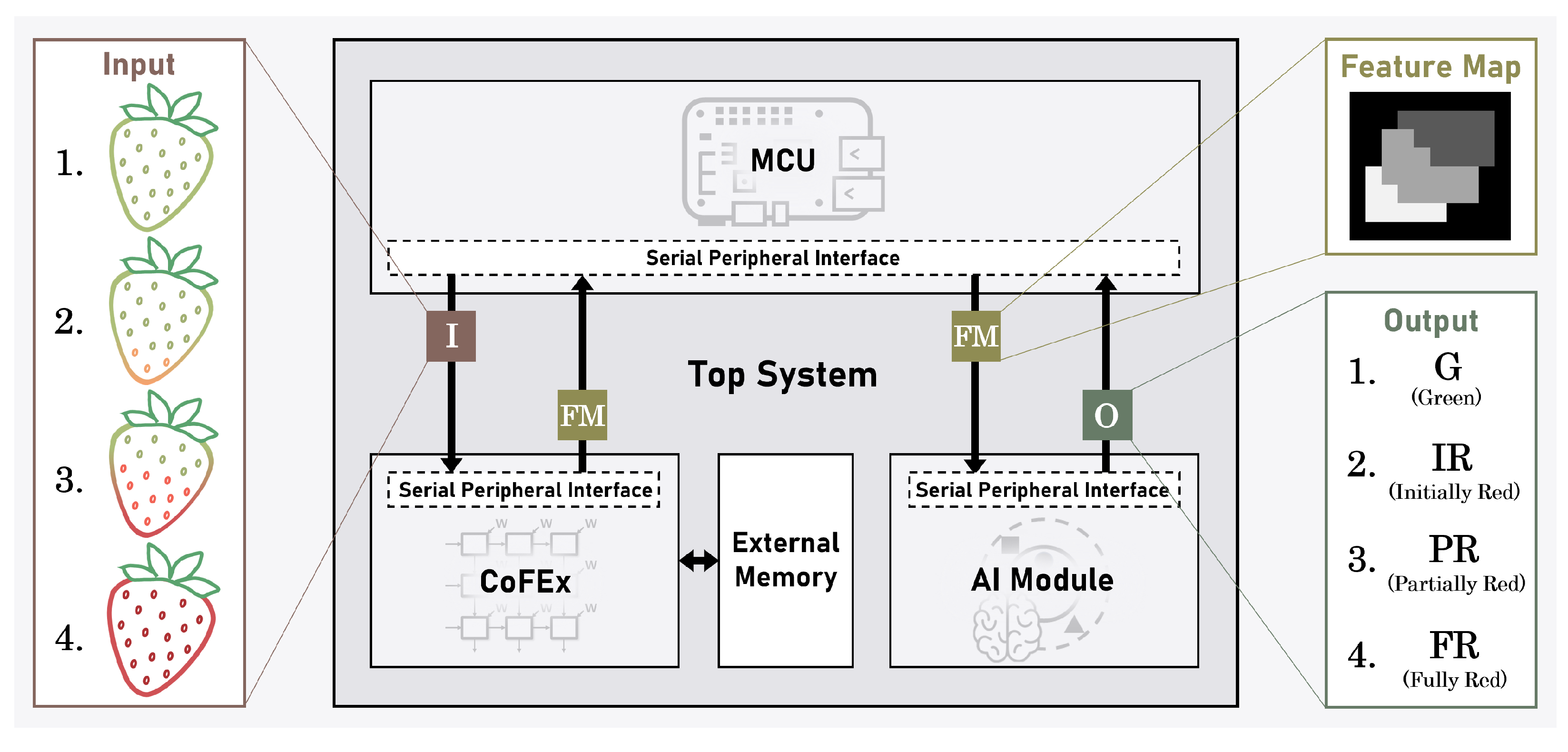
Figure 1 illustrates the overall system architecture that we propose for classifying multi-channel strawberry images according to their ripeness. The proposed system consists of the CoFEx, which extracts features; the Intellino, an edge AI processor based on the k-NN algorithm for classifying ripeness utilizing the extracted feature mapsl; and the micro controller unit (MCU), which controls the CoFEx and the AI processor. The MCU communicates with both the CoFEx and the AI processor through the synchronous serial communication protocol, serial peripheral interface (SPI), controlling the learning and inference states of both modules. Furthermore, the external memory serves as a repository for extensive parameters and feature map data, supplying them to the CoFEx as required.

The CoFEx accelerates the convolution layer operations of a pre-trained CNN model, efficiently extracting features from strawberry images. The extracted feature maps are provided as input to the AI processor, Intellino. The AI processor based on the k-NN algorithm classifies the ripeness of strawberry images into categories such as ‘Green’, ‘Initially Red’, ‘Partially Red’, and ‘Fully Red’. The MCU utilizes SPI communication to transmit pre-trained CNN model parameters and layer information to the CoFEx according to predetermined instructions. Additionally, the MCU conveys the feature map data extracted by the CoFEx to the Intellino to determine the ripeness of strawberries. Through this, a harmonious interaction among the CoFEx, the AI processor, and the MCU is achieved, enabling the effective operation of the entire system.

3.1. CoFEx

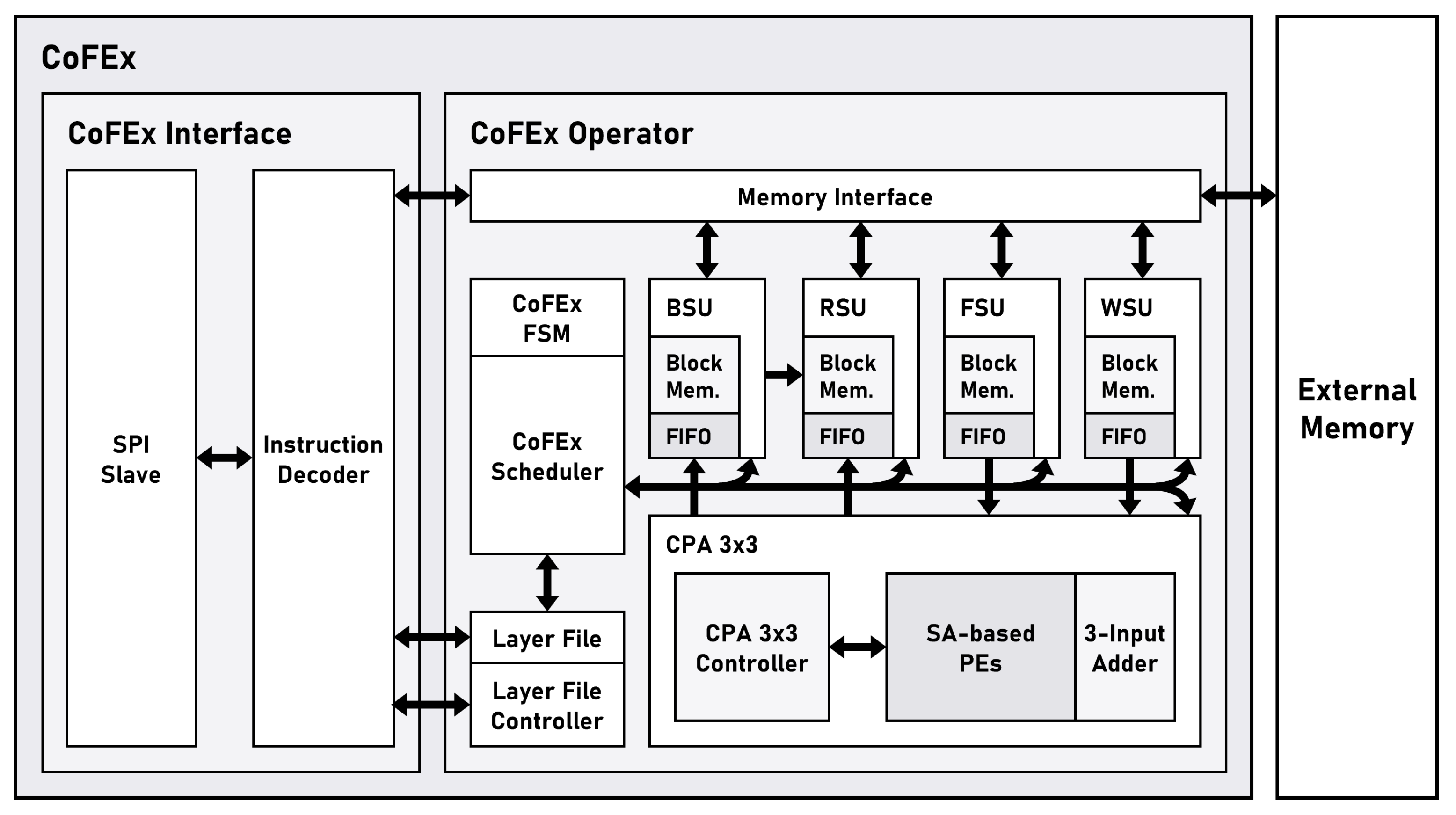
Figure 2 shows the block diagram of the CoFEx. The CoFEx is broadly divided into the CoFEx Interface section and the CoFEx Operator section. The CoFEx Interface section is comprised of an SPI Slave, responsible for communication with the external system, and an Instruction Decoder that interprets commands received through SPI communication. Through this, the Interface section efficiently communicates with the external system and processes commands. The CoFEx Operator section includes a Layer File for storing CNN model layer information and a Layer File Controller to ensure that layer information is stored and operates in the correct order. Furthermore, the Operator section comprises the CoFEx Scheduler to control operations related to the required convolution layer, a convolution processing accelerator3x3 (CPA3x3) for performing convolution operations, and various setup units to configure parameters and result data appropriately in different situations.

The Layer File contains various information related to each layer of the CNN model received through instructions. The information for each layer, including address pointers for weight, bias, feature map, and result, is flexibly modified by the user as needed through instructions. This allows for adaptability to various CNN models, enabling swift adjustments to changes in the model. The CoFEx Scheduler, based on the information from the layer file, determines the operational status of various functions. Additionally, the CoFEx Scheduler, driven by an internal state machine, enables each setup unit and convolution accelerator to operate sequentially. The CPA3x3, a critical component of the CoFEx, efficiently performs the frequently used 3 by 3 convolution operations in CNN models. The CPA3x3 consists of a CPA3x3 Controller, SA-based processing elements (PE), and a 3-Input Adder that sums the results outputted from the PEs. The CPA3x3 Controller regulates the movement of input and output as well as internal partial sum data within the accelerator to ensure the smooth operation of the dataflow in the SA. The SA-based PEs have a specialized architecture tailored for nine-sized weights, with all internal PE statically arranged to support high-speed convolution operations. The 3-Input Adder simultaneously adds three 32-bit floating-point data outputs generated by the PEs.

The bias setup unit (BSU), the result setup unit (RSU), the feature map setup unit (FSU), and the weight setup unit (WSU) are controlled by the CoFEx scheduler. These setup units efficiently set the data required for convolution layer operations. Additionally, the setup units fetch information from external memory, store it in internal block memory, and transmit data from the CPA3x3 utilizing first-in first-out (FIFO) under appropriate circumstances. The data are received from the CPA3x3 as needed. Finally, the Memory Interface, through the Instruction Decoder, either directly transfers data like parameters to External Memory or fetches data from External Memory in block units as required by the setup units. This approach allows the setup units to efficiently manage data, and facilitates effective data transfer between external memory and the accelerator, supporting optimal system operation.

3.1.1. Finite-State Machine of the CoFEx

The CoFEx is designed to efficiently handle diverse functionalities required in convolution layer, encompassing not only convolution operations but also various functions like zero padding, max pooling, bias addition, and activation function. These various functionalities are operationalized by the CoFEx FSM implemented within the CoFEx scheduler, based on the configuration information of each layer stored in the Layer File. The CoFEx FSM governs CPA3x3 and setup units to facilitate the sequential execution of individual functionalities.

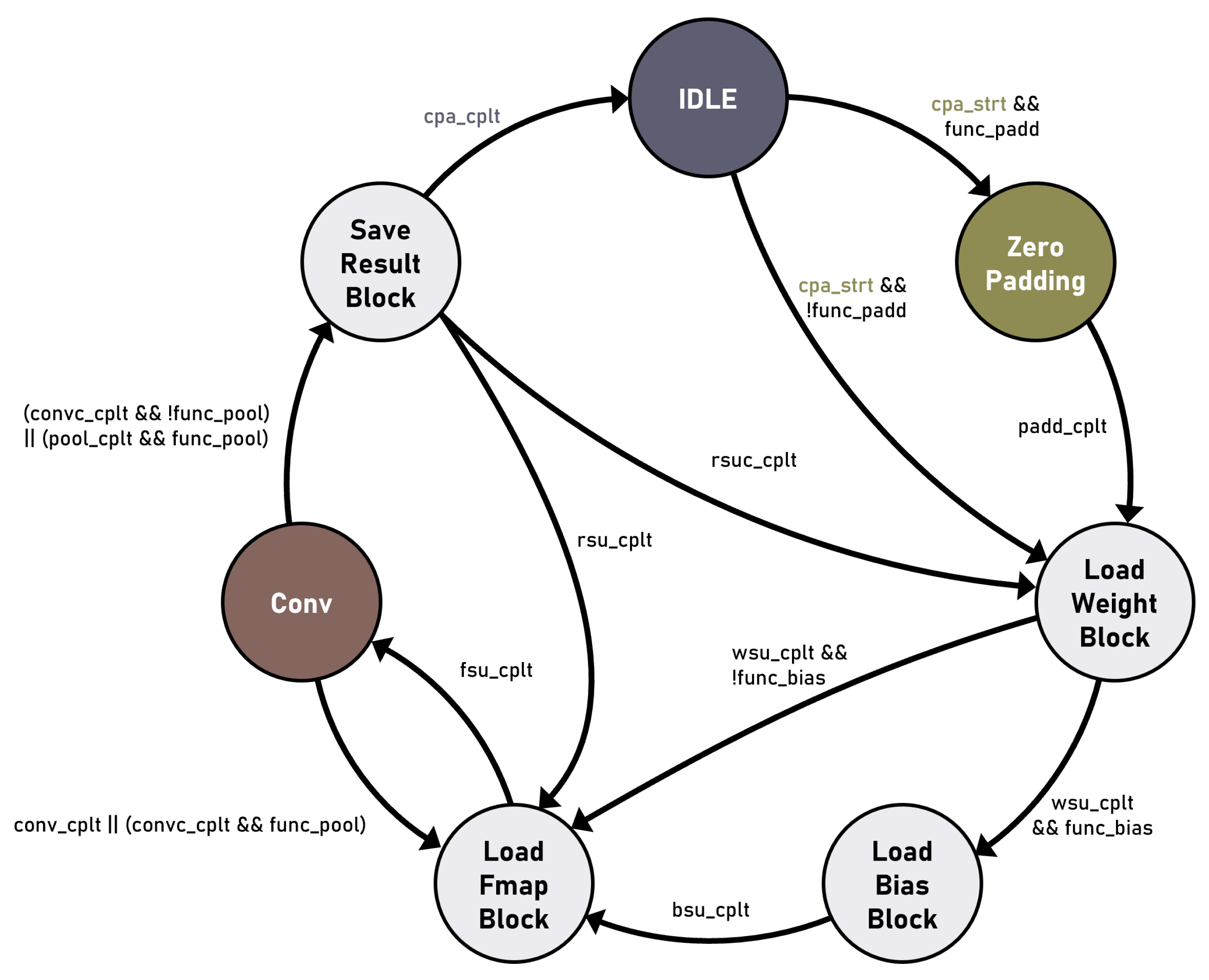
Figure 3 represents the architecture of the CoFEx FSM. && represents and operation, and || represents or operation as logical operators. Before the operation commences, the CoFEx Scheduler sets the state of various function bits based on the layer configuration information stored in the Layer File. The function bits include func_padd, func_bias, and func_pool. These bits indicate whether zero-padding is performed, whether bias is used, and whether the max-pooling function is activated, respectively.

In the initial state, zero-padding is determined based on the cpa_strt signal and the func_padd bit. Upon performing zero-padding, zero data are added to the feature map data at both the front and back before being inputted into CPA3x3. Subsequently, as the operation progresses, in the load weight block (LWB) state, the WSU loads a weight block of input channel size from external memory. Moreover, depending on the state of the func_bias bit, the BSU either fetches the bias block or progresses to the load fmap block (LFB) state. In the LFB state, the FSU fetches one channel data from the input channels of the feature map in blocks, starting from the top three rows. Following that, in the conv state, convolution operations are performed on the portions corresponding to the top three rows. If the func_pool state is not ‘1’, the CoFEx FSM reverts to the LFB state to fetch the feature map block of another single channel. Upon completing the partial convolution operation for the input channels utilizing this method, the conv_cplt signal is generated, and the FSM transitions to the save result block (SRB) state. In the SRB state, the RSU transfers the computation results to external memory. As the convolution for the input channels is not yet completed, FSM returns to the LFB state based on the rsu_cplt signal. Subsequent to the completion of convolution operations for all input channels, the transition to the LWB state is triggered by the rsu_cplt signal. The WSU loads the weight block corresponding to the next input channel size, and this iterative process continues. Furthermore, upon the completion of convolution operations for all input channels, a return to the IDLE state is triggered by the cpa_cplt signal.

In the func_pool state was ‘1’, the iterative sequence of the CoFEx FSM undergoes a slight modification. The convolution operation for a single channel continues to iterate until the pool_cplt signal occurs, regardless of the completion of partial convolution for that channel. In the iterative operation process, for the purpose of max pooling, the larger data are selectively stored in the temporary register inside the RSU by comparing the sizes of data in pairs. This process repeats twice, and the results are compared with the data stored in the temporary register inside the RSU. The larger data are then saved again in the temporary register. The data stored in the temporary register undergo a transition to the SRB state following the pool_cplt signal, facilitating the RSU in transmitting the respective data to the external memory.

3.1.2. Systolic Array Architecture of PEs

In DL models, a large number of repetitive convolution operations are performed to effectively extract feature maps from multichannel images. In particular, these convolution operations are crucial for detecting and extracting various features in large-scale image datasets. Convolution operations require repetitive multiplication and addition, making bottleneck issues prone to occur in traditional von Neumann architectures. To overcome these limitations, SA is gaining attention for its effective hardware acceleration structure in DL models, maximizing parallelism and efficiently processing diverse matrix operations at high speeds [26,36]. Therefore, we accelerated the convolution operations performed in the CoFEx by leveraging the SA architecture.

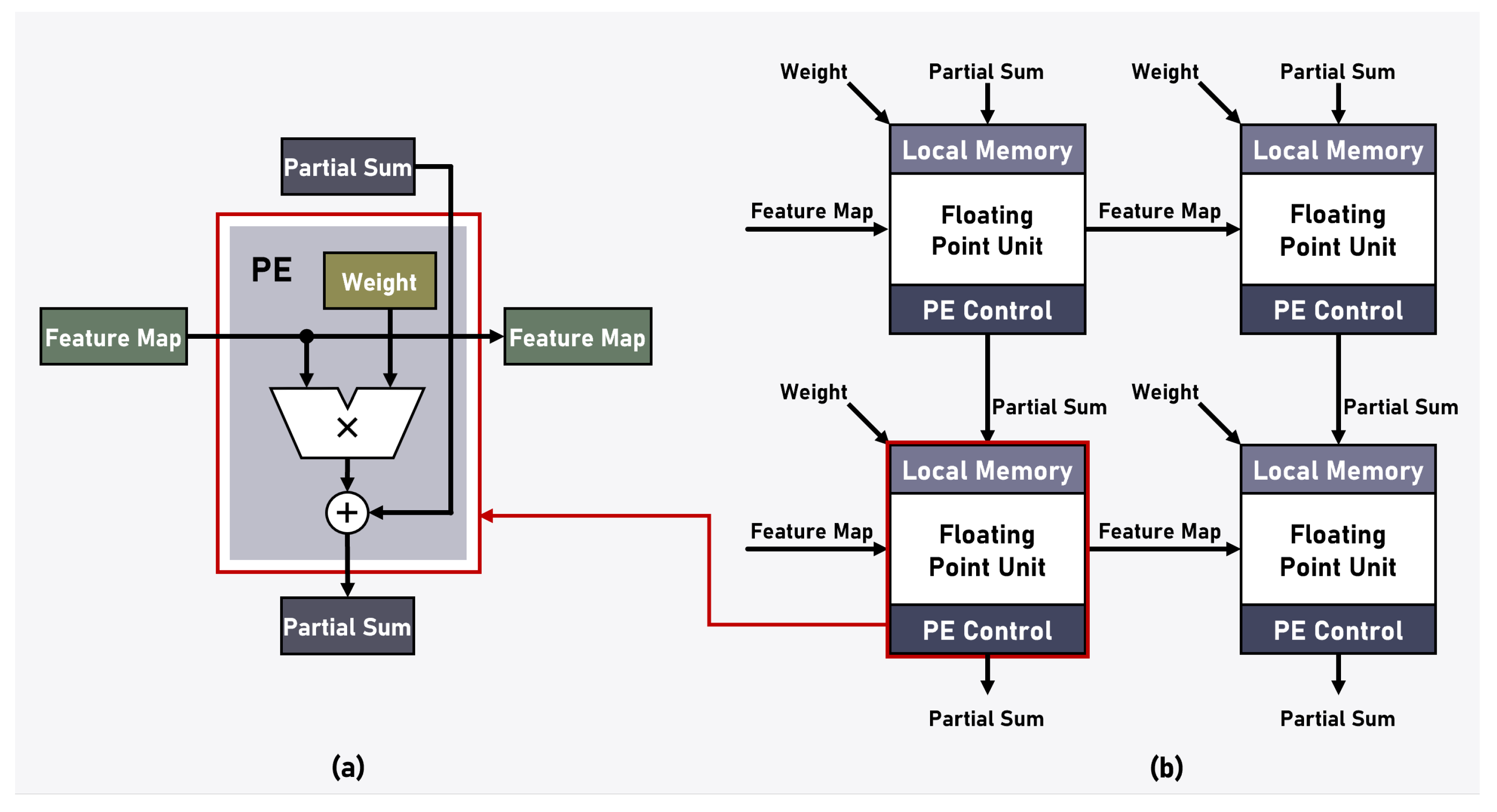
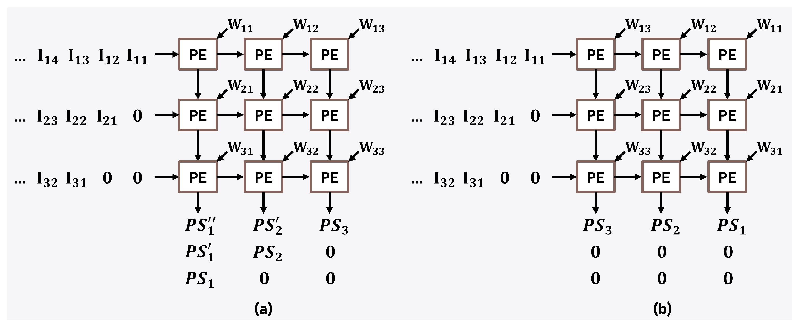
The SA architecture is organized with PE arranged in a regular array, where each PE cell operates in parallel, systematically processing specific portions of the matrix. Figure 4 illustrates the arrangement of PE and the overall SA architecture in our proposed system. Each PE stores weight values internally in advance and performs multiplication operations as needed with input feature map data. Furthermore, the results of the multiplication operations are combined with partial sums generated by neighboring PEs through addition, and then communicated back to the surrounding PEs. Both the multiplication and summation operations within the PE adhere to IEEE-754 half-precision floating-point arithmetic, utilizing 32-bit precision.

The SA architecture is a specialized form of data processing where multiple data elements move simultaneously in a specific direction, and each PE along the path performs the same operation in parallel. This architecture allows for efficient reuse of data according to the dataflow, minimizing computational bottlenecks and achieving high performance. Especially in SA, various dataflow methods exist, with weight stationary (WS), output stationary (OS), and input stationary (IS), among others, being representative examples [37]. These dataflow methods differ in how operations are conducted based on the movement of data. WS denotes the method in which data move while weights are fixed, OS denotes the method in which data move while output is fixed, and IS denotes the method in which data move while input is fixed. Selecting the suitable method from these diverse dataflow approaches is a key strategy in crafting an SA architecture optimized for specific operations.

Figure 5 illustrates the dataflow of the SA used in our proposed system, as well as the dataflow of the conventional WS method. The proposed dataflow, an improved version of the traditional WS method, is specifically optimized for convolution layer operations. By storing the weights from the opposite end of the feature map input, the operation, facilitated by the SA, systematically produces results consecutively along a specific column direction. The proposed dataflow enhances performance by minimizing clock waste at the input and output stage of the SA. Furthermore, we added a three-input adder to the output stage of the SA architecture, combining the output of three partial sum results before the final output. This dataflow enables the CoFEx to process convolution layer operations more efficiently and continuously.

3.2. AI Processor, Intellino

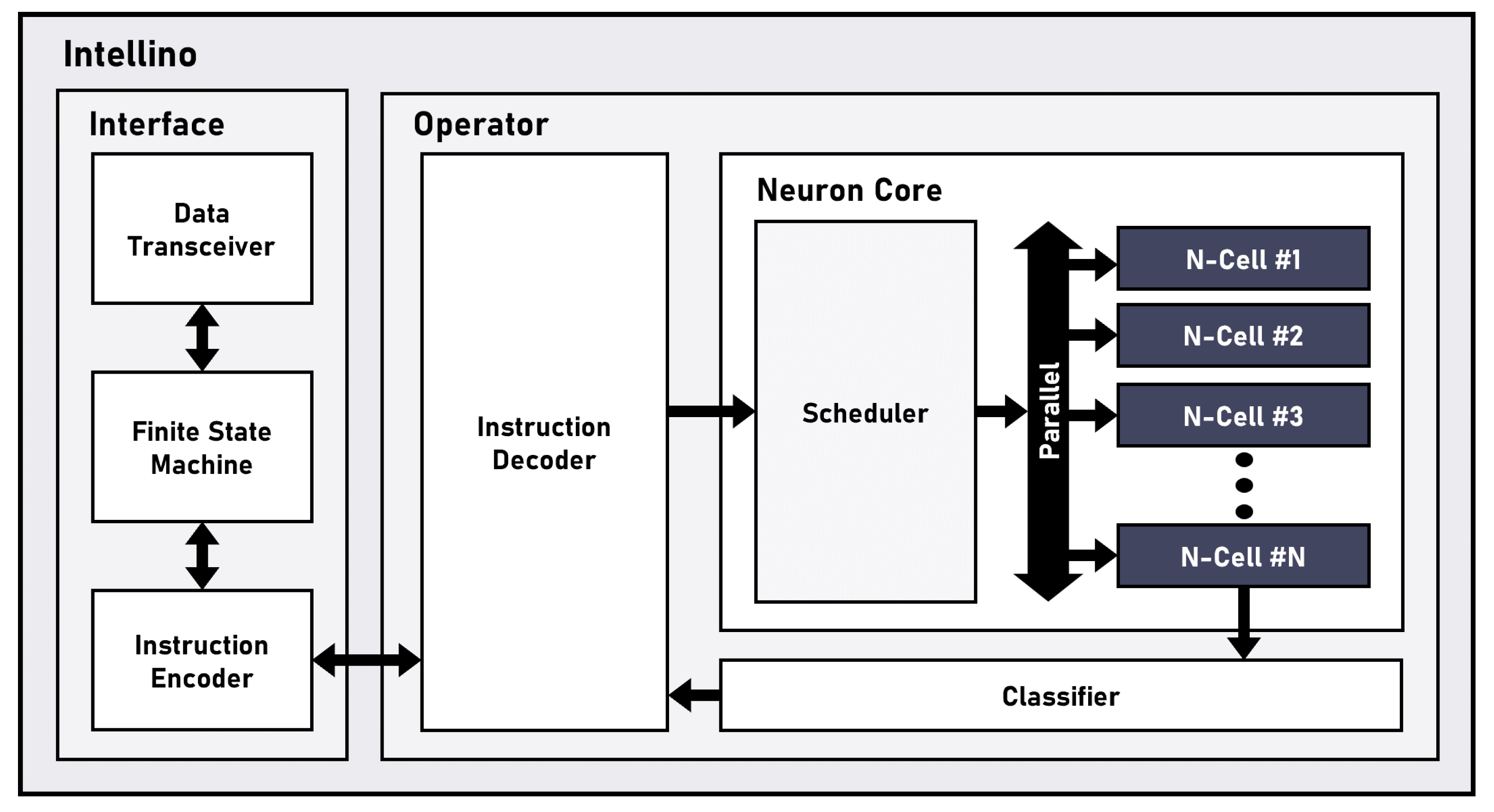
Figure 6 illustrates the architecture of the AI processor, Intellino, employed in the proposed system [38]. The Intellino is an AI processor designed for embedded systems, featuring low power consumption and efficient resource utilization based on the k-NN and radial basis function-neural network (RBF-NN) algorithms. The architecture employs parallelized neurons in a single neural network, enabling simultaneous and efficient large-scale recognition while reducing the workload on the system.

The AI processor, Intellino, comprises the Interface and Operator components. The Interface, facilitating data exchange with external sources, consists of the Data Transceiver, the finite-state machine (FSM), and the Instruction Encoder. The Data Transceiver receives datasets for learning and recognition or instructions from external sources. The FSM interprets the received data according to a specific protocol. The Instruction Encoder encodes interpreted data and transmits the encoded information to the Operator. The Operator, consisting of the Instruction Decoder, Neuron Core, and Classifier, performs learning and recognition tasks based on the input data. The Instruction Decoder processes encoded information, including data, category, distance, write and read signals, and algorithm details, directing the operation of the Neuron Core accordingly. The Neuron Core comprises a Scheduler and parallel-connected Neuron-cells(N-cell). Each N-cell has a vector memory, storing training data and corresponding categories during learning. In recognition tasks, the Neuron Core computes the distance between the input data and the data stored in the vector memory of each N-cell. This distance calculation is performed for all trained N-cells, and the results are sent to the Classifier. The Classifier, using the user-selected k-NN or RBF-NN algorithm, determines the category of the input data based on the N-cell with the smallest distance. As the number of N-cells increases, the required number of memory also significantly grows. Therefore, the selection of an appropriate vector size and N-cell count depends on the data size of the desired model and hardware design specifications.

However, the AI processor, Intellino, has limitations in terms of the number of N-cells required to train a large amount of data, limiting the quantity of learnable data. Therefore, efficient utilization of memory size through effective learning is crucial. The AI processor exhibits limitations in handling continuously evolving data over time due to the absence of parameters capturing the temporal correlation between past and present input data. Hence, for sequential data classification such as sound analysis, preprocessing methods are crucial, and the classification performance is significantly influenced by how preprocessing is conducted [39,40]. The AI processor, which excels in the classification of single-channel vector data, is well-suited for creating classification models through image processing, such as determining parking feasibility and detecting human movement, leveraging the advantages of k-NN [41,42]. But, the AI processor is disadvantageous in directly analyzing and classifying information from multichannel input data. In this paper, to overcome the limitations of the AI processor, we trained and inferred the AI processor utilizing only the feature map data extracted through the convolutional operations-based CNN model. Through this approach, we effectively acquired a training dataset, reduced the memory requirements for the AI processor’s learning process, and enhanced the inference performance for multichannel images.

4. Implementation and Analysis

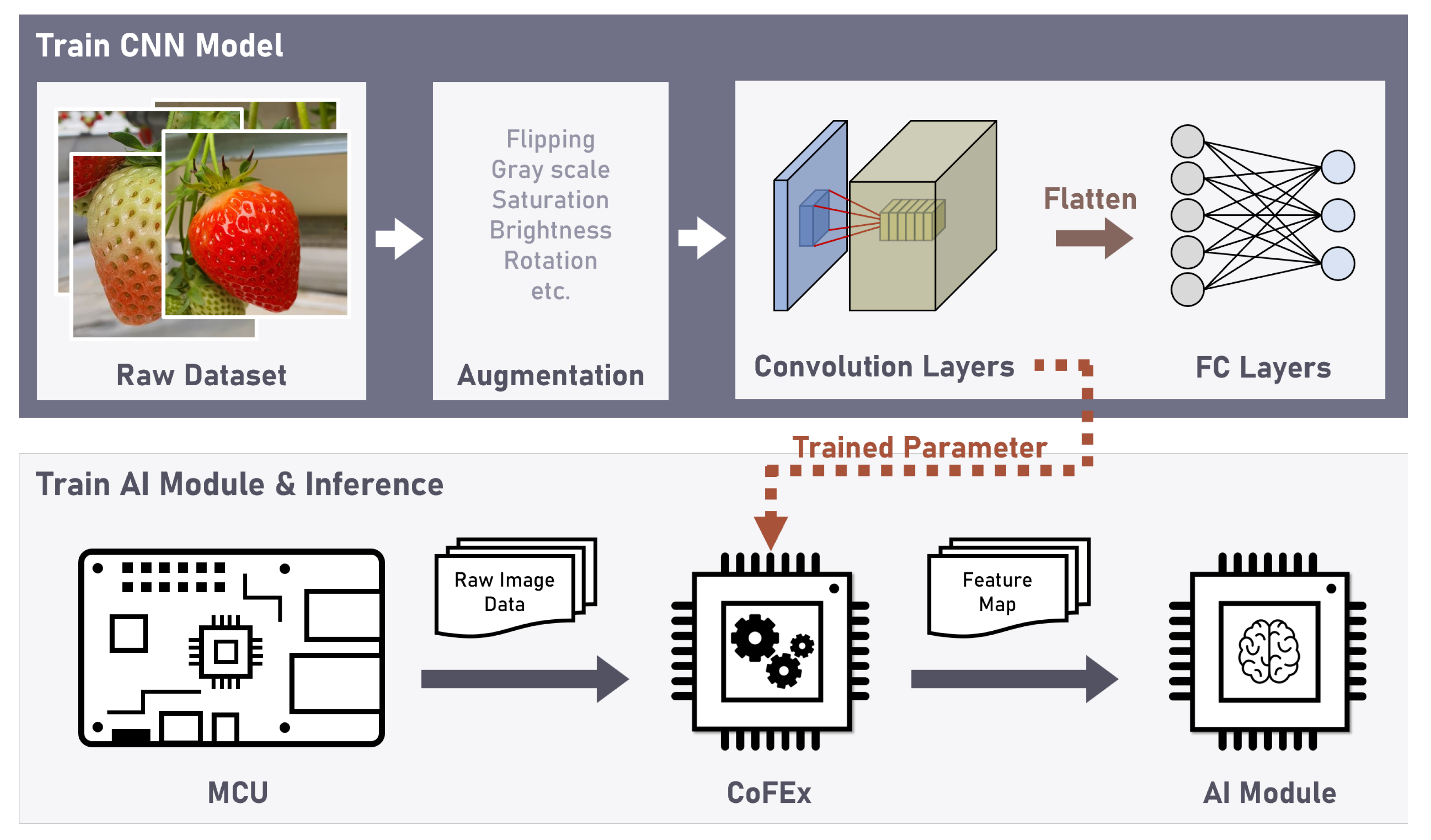
To assess the performance of the proposed system without causing any harm to the actual system, we initially conducted software simulations by simulator before proceeding with the implementation [43]. We subsequently implemented a strawberry ripeness classification system incorporating the CoFEx and the AI processor, Intellino. Figure 7 illustrates the overall system flow, encompassing parameter learning, parameter setting, feature extraction, and result inference. We curated a dataset for training and inference purposes by directly capturing strawberry images from agricultural settings. We directly gathered strawberry images from a strawberry farm and curated a dataset for training and inference purposes. The gathered strawberry image dataset was categorized into four classes based on ripeness: ‘Green’, ‘Initially Red’, ‘Partially Red’, and ‘Fully Red’, comprising 829, 171, 90, and 871 images, respectively.

Data augmentation is an essential method to overcome the performance degradation caused by limited datasets and to avoid over-fitting [44]. Employing data augmentation techniques, we expanded the dataset to a total of 18,000 instances. We utilized the OpenCV library to perform augmentation techniques on images, including flipping horizontally and vertically, rotating randomly within the range of −30 to 30 degrees, and adjusting brightness. These image augmentation techniques were applied randomly to enhance the dataset, and multiple augmentations were applied to each image. The augmented images were segregated into two distinct sets for experimentation, 8000 images for training the CNN model and the AI processor, and an additional 10,000 images dedicated to feature extraction and result inference.

In the process of training CNN model, we employed the PyTorch library, a Python-based open-source machine learning framework, to train a CNN model with appropriately designed layers. The trained CNN model utilized kernels to extract feature maps. Subsequently, we applied the layer information and parameter data from the trained model’s convolution layer to the CoFEx. In the process of training Intellino, we initiated the procedure by randomly selecting data from the training dataset, which was originally utilized for training the CNN model. The selection of data was based on the required number of cells that the AI processor would be trained on. The CoFEx with appropriate layer information extracted feature maps in 32-bit floating-point format. The extracted map data were quantized into an 8-bit integer format and applied to the training of the AI processor as a one-dimension feature vector. In the inference process, we utilized the test dataset to perform the same quantization of the feature map data extracted from the CoFEx into an 8-bit feature vector. Subsequently, the AI processor inferred the strawberry ripeness classification category based on this vector.

4.1. Implementation

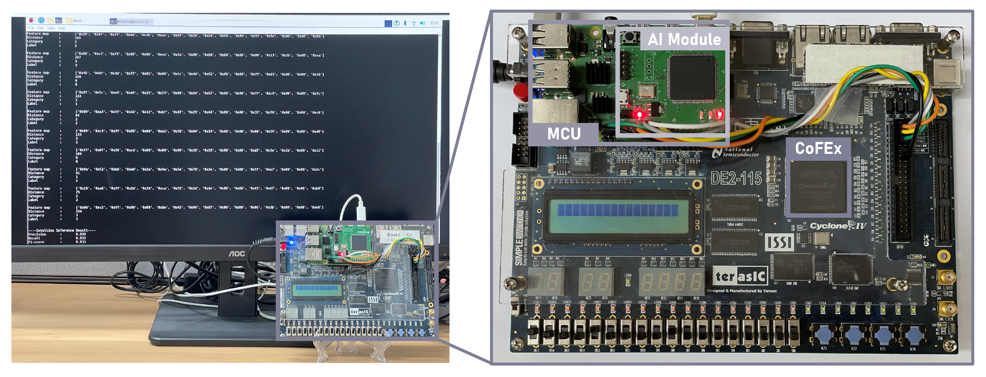
Figure 8 illustrates the hardware experimental environment for our proposed strawberry classification system. The proposed system consists of the CoFEx, the AI processor Intellino, and an MCU. We implemented the CoFEx on the Intel FPGA (Cyclone IV: EP4CE115F29C7N) embedded in the development board, and implemented the AI processor on the Intel FPGA (MAX 10: 10M50SAE144C8G). The CoFEx and AI processor were designed utilizing Verilog HDL. Both modules are interfaced with the MCU through general purpose input/output (GPIO), and communication with the MCU is established using the SPI protocol. Also, we employed a Python-based simulator to conduct simulations under various conditions for constructing a system model suitable for strawberry ripeness classification. Through the simulator, we conducted a performance analysis of the classification system based on the layer configuration of an appropriate CNN model and the memory size of the AI processor. Leveraging the system under optimized conditions, we conducted functional validation of the strawberry ripeness classification system utilizing feature maps in the implemented environment.

To validate the functionality, we pre-emptively applied the suitable CNN modeled system, obtained through simulation, into the implemented hardware system and proceeded with experiments. The proposed system was trained and inferred on four categories of strawberry ripeness, ‘Green’, ‘Initially Red’, ‘Partially Red’, and ‘Fully Red’. The inference results included the feature map data information list extracted through the CoFEx, the distance result value and the category value from the AI processor, and performance metrics such as the F1 score. We validated the utility of our system by the performance metrics and the memory size used during the inference process. Furthermore, we confirmed that the CoFEx, which bears a substantial computational load, has an operation processing time of 495 milliseconds at a clock speed of 50 MHz. Additionally, the total execution time of our proposed system took 533 milliseconds, during which the input image passed through the CoFEx to generate a feature vector, traversed MCU, and was transmitted to the AI processor for the inference of ripeness.

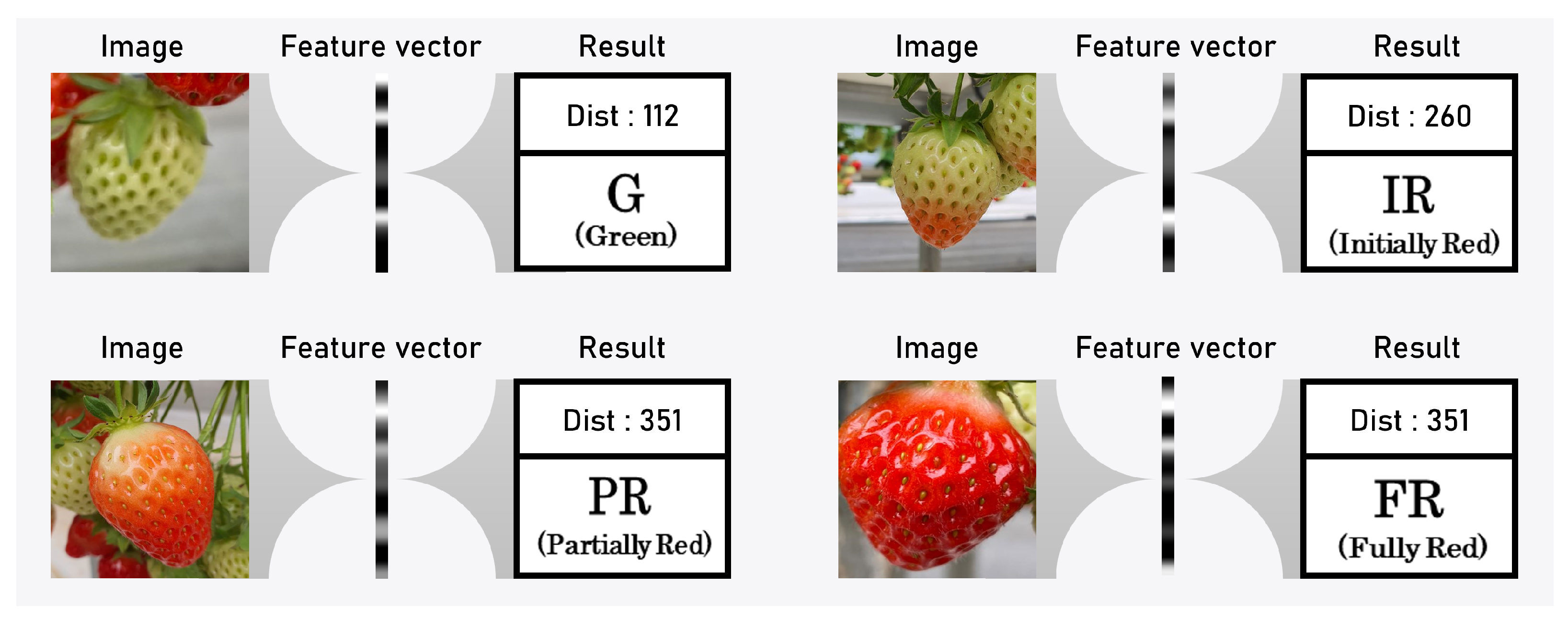
Figure 9 illustrates the result of the implementation of the input images for inference, the feature vector extracted through convolution layer operations, and the classified results. All input images have undergone the data augmentation process. The size of the extracted feature vector is 16, and this vector is input into the k-NN algorithm. Ultimately, the ripeness is determined by classifying the category associated with the closest distance value obtained through a simple subtraction operation.

4.2. Analysis

The performance assessment of our proposed strawberry ripeness classification system involved evaluating its suitability through key performance metrics, namely the average precision, recall, and F1 score for each classification category. Equation (2) represents the formula for calculating the F1 score. Precision is the proportion of true positive (TP) samples among those predicted as positive, with a focus on minimizing false positives (FP). Recall represents the proportion of TP samples among those that are actually positive, emphasizing the reduction of false negatives (FN).

$$\mathrm{F}1\mathrm{score}=2\times \frac{\mathrm{Precision}\times \mathrm{Recall}}{\mathrm{Precision}+\mathrm{Recall}}$$

(2)

The F1 score is a metric that measures how harmoniously precision and recall are combined through their harmonic mean. Additionally, the F1 score measures how accurately the positive class is identified and how well the model detects samples belonging to the positive class. Therefore, we conducted an analysis of our system’s performance in specific contexts based on these metrics.

4.2.1. Comparison Based on Model Depth and Thickness

To analyze the proposed system, we conducted experiments based on the depth and thickness of CNN model layers, as well as analyses of memory size and computational methods. Firstly, we divided the models based on the depth of the network, with a relatively deep CNN model (Model5) composed of five convolution layers and a relatively shallow CNN model (Model4) composed of four convolution layers. Furthermore, each experimental model was separated into three categories; the Fat model, which has operations for a relatively large number of channels; the Normal model, with an intermediate number of channels; and the Thin model, with fewer channels. 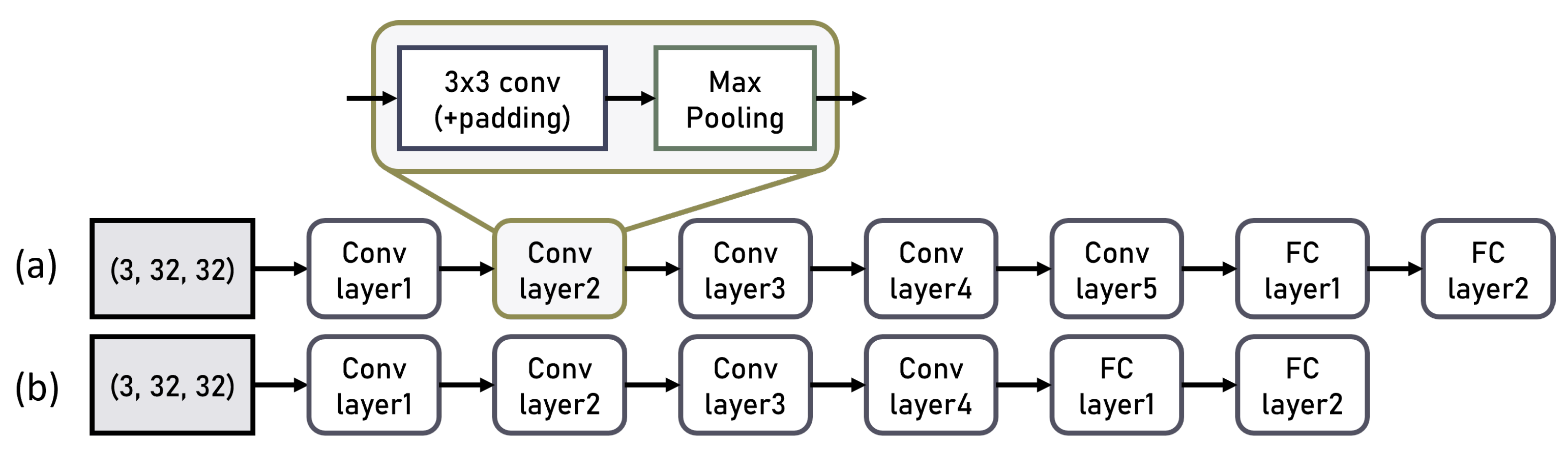Figure 10 shows the architecture of Model5 and Model4 and

Table 2. The input/output channel configurations in Model5 and Model4.

Channel: (Input, Output)		Layer1	Layer2	Layer3	Layer4	Layer5
Model5	Fat	(3, 16)	(16, 16)	(16, 16)	(16, 16)	(16, vector size)
	Normal	(3, 8)	(8, 16)	(16, 16)	(16, 8)	(8, vector size )
	Thin	(3, 8)	(8, 8)	(8, 8)	(8, 8)	(8, vector size)
Model4	Fat	(3, 16)	(16, 16)	(16, 16)	(16, vector size)	-
	Normal	(3, 8)	(8, 16)	(16, 16)	(8, vector size)	-
	Thin	(3, 8)	(8, 8)	(8, 8)	(8, vector size)	-

provides detailed information about the input and output channel configurations for each layer in Model5 and Model4, categorized by their thickness.

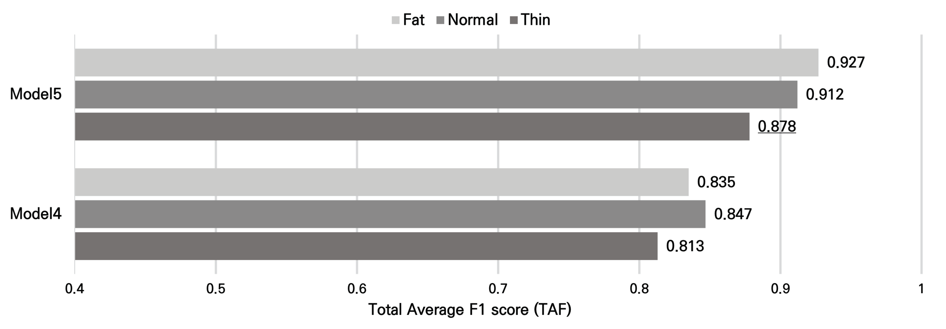
To assess the comparative performance of the models, we conducted an evaluation based on the total average F1-score (TAF) metric. The TAF represents the average F1 score for each model, ranging from 4 to 2048 cells and with vector sizes varying from 4 bytes to 64 bytes. Figure 11 shows the TAF values corresponding to the structures of each model. The relatively deep Models5 generally achieved TAF values of 0.9 or higher, while the comparatively shallow Model4 had a maximum TAF of around 0.85. Additionally, Model5 showed approximately 7% to 11% higher TAF compared to Model4 under similar conditions. Hence, we concluded that deeper models are more meaningful. Within Model5, a comparison of TAF values based on channel thickness, the Fat model with thicker channels exhibited a relatively higher TAF value of 0.927 compared to the Normal and Thin models with relatively thinner channels. In conclusion, we determined that the Model5-Fat is the most suitable model.

4.2.2. Comparison According to Model Memory Size

Table 3. Model5-Fat results.

Model5-Fat														Average F1 Score (Vector)
			Number of Cell										FC layer
			4	8	16	32	64	128	256	512	1024	2048	Parameter
Vector Size	4	Memory	16	32	64	128	256	512	1024	2048	4096	8192	1176	0.919
		Precision	84.5%	92.2%	92.3%	92.9%	93.1%	92.9%	93.1%	92.9%	92.9%	93.2%
		Recall	83.6%	91.6%	92.2%	92.8%	93.0%	92.7%	93.0%	92.9%	92.8%	93.1%
		F1 score	0.840	0.919	0.922	0.928	0.930	0.928	0.930	0.9229	0.928	0.931
	8	Memory	32	64	128	256	512	1024	2048	4096	8192	16,384	1512	0.929
		Precision	86.5%	91.5%	92.8%	93.2%	94.2%	94.2%	94.5%	94.5%	94.6%	94.6%
		Recall	85.5%	90.4%	92.4%	92.7%	94.1%	94.1%	94.4%	94.5%	94.4%	94.5%
		F1 score	0.860	0.909	0.926	0.929	0.941	0.941	0.944	0.945	0.945	0.945
	16	Memory	64	128	256	512	1024	2048	4096	8192	16,384	32,768	2184	0.933
		Precision	90.1%	93.4%	89.9%	91.4%	94.2%	95.0%	95.1%	95.3%	95.3%	95.1%
		Recall	88.8%	93.3%	88.7%	90.7%	94.2%	95.0%	95.1%	95.2%	95.2%	95.0%
		F1 score	0.894	0.933	0.893	0.910	0.942	0.950	0.951	0.952	0.952	0.950
	32	Memory	128	256	512	1024	2048	4096	8192	16,384	32,768	65,536	3528	0.920
		Precision	87.8%	89.4%	92.7%	92.3%	92.0%	93.3%	93.7%	93.9%	93.9%	93.7%
		Recall	86.9%	89.0%	92.2%	91.4%	91.4%	92.9%	93.4%	93.8%	93.8%	93.5%
		F1 score	0.873	0.892	0.924	0.918	0.917	0.931	0.935	0.938	0.938	0.936
	64	Memory	256	512	1024	2048	4096	8192	16,384	32,768	65,536	131,072	6216	0.933
		Precision	90.0%	91.9%	92.5%	92.6%	93.8%	94.5%	94.8%	94.7%	94.7%	94.5%
		Recall	89.5%	91.6%	92.0%	92.0%	93.7%	94.4%	94.7%	94.7%	94.6%	94.5%
		F1 score	0.897	0.917	0.922	0.923	0.937	0.944	0.947	0.947	0.946	0.945
Average F1 score (Cell)			0.873	0.914	0.918	0.922	0.934	0.939	0.942	0.942	0.942	0.942	TAF:0.927

for experimental results show Memory, Precision, Recall, and F1 score for various quantities of cells ranging from 4 to 2048 and vector sizes from 4 to 64 bytes. In this case, Memory refers to the memory required for the AI processor, specifically the product of the cell and vector sizes. Additionally, Precision, Recall, and F1 score refer to precision, recall, and F1 score under the specified conditions. The vector size is associated with the extracted feature map and later with the number of parameters in the FC layer constructed afterward. Therefore, we represented the number of parameters in FC layers as FC layer parameter. Additionally, we conducted experiments based on CNN models that were appropriately trained and achieved an F1 score of 0.9 or higher. In the endeavor to minimize the memory footprint essential for constructing the AI processor, our concentration was directed towards conditions exhibiting a superior F1 score compared to TAF, with particular emphasis on the smallest memory size. Considering the TAF of 0.927 for the selected Model5-Fat, we explored conditions that achieve a higher F1 score than TAF. Therefore, we considered the model with the highest F1 score among conditions with a 128 byte memory size, characterized by 8 cells and a 16 byte vector, as the optimal configuration. This memory optimization selection allows for maintaining high accuracy while utilizing fewer memory resources and performing fewer computations.

In the optimal model, we utilized a lightweight algorithm-based AI processor, specifically based on the k-NN algorithm, instead of performing multiplication operations for the extensive parameters in the FC layer. The lightweight k-NN algorithm utilized in the AI processor performs distance-based computations utilizing only addition and subtraction operations. We replaced the FC layer operations, containing 2184 parameters and performing over 2000 multiply–accumulates (MAC), with a k-NN operation that requires only 128 bytes of memory and performs just 128 subtraction operations. We efficiently utilized resources by performing fewer operations compared to the traditional FC layer, which involves a significant number of multiplication and addition operations. Through this approach, we achieved high performance with a relatively small memory resource of 128 bytes, showcasing a precision of 93.4%, recall of 93.3%, and an F1 score of 0.933.

4.2.3. Comparison to Similar Research and Algorithm

Table 4. Comparison to similar research.

	[31]	[32]	[33]	[34]	[35]	[Intel Core i7-12700 (2.10 GHz)]
						k-NN	MobileNet	Our
Parameters	6.2 M	16.1 M	-	-	2.01 M	128	3.22 M	0.01 M
Accuracy	95%	90.33%	85%	85.64%	88.57%	32.1%	97.92%	93.3%
Run Time	60 ms	-	-	-	23 ms	0.03 ms	39 ms	0.91 ms

presents the classification accuracy, parameter number for operations, and execution time for strawberry ripeness in several similar studies [31,32,33,34,35], as well as representative lightweight algorithms such as k-NN and MobileNet, and our system. The number of parameters used in operations is closely related to the computational capabilities of each system. As the number of parameters required for operations increases, more memory resources are needed, leading to increased external memory access and a decrease in computational performance. Moreover, the number of operations that need to be performed also increases proportionally to the parameters. From this perspective, our proposed system has a parameter count of 0.01 M, significantly fewer parameters compared to similar studies, providing an advantage in computational performance. Additionally, with a relatively high accuracy of 93.3%, our system demonstrates the ability to achieve sufficiently high accuracy while using fewer memory resources compared to other similar studies.

Moreover, we conducted comparative experiments in the same Intel Core i7-12700 (2.10 GHz) environment to compare the execution speed of our system with representative lightweight algorithms, k-NN, and MobileNet. The k-NN algorithm, with very few parameters, performed at a very fast speed. But the accuracy of the k-NN algorithm was relatively low, not sufficiently validating its utility. MobileNet exhibited a high accuracy of 97.92%. However, due to over 30,000 parameters, MobileNet required significantly more memory resources than our algorithm, resulting in a much slower execution speed. Therefore, through these comparisons, we confirmed that our system demonstrates sufficiently high accuracy despite using very little memory.

5. Conclusions

In this paper, we proposed a strawberry ripeness classification system utilizing the CoFEx and the lightweight algorithms based AI processor, Intellino. The proposed system consists of the CoFEx, which extracts suitable feature maps from RGB 3-channel strawberry images, the Intellino, an edge AI processor utilizing the extracted feature maps for strawberry ripeness classification, and the MCU, which controls and operates the entire system. We utilized the Python environment and the PyTorch library to train a CNN model suitable for the strawberry classification system. Subsequently, we applied the parameter information from the convolution layer of the appropriate CNN model to the CoFEx. The appropriately sized feature map outputted from the CoFEx was then input into the AI processor, Intellino, for training and inference. We implemented the CoFEx and the AI processor utilizing FPGAs named Cyclone IV and MAX 10, respectively. These two modules communicate through the MCU utilizing the SPI protocol, exchanging input and output, parameter information, and control information. Furthermore, we designed and validated both modules with Verilog HDL.

To evaluate the efficiency of our proposed system, we conducted experiments varying the layer depth and channel width of the CNN model, as well as the memory size of the AI processor. We utilized the F1 score, which represents the harmonic mean of precision and recall, as the metric for our analysis. To compare the performance based on the depth and channel thickness of the models, we evaluated the TAF. We selected the Model5-Fat, which exhibited the highest TAF, as the most suitable model. Within the context of the Model5-Fat, we conducted a performance analysis by varying the vectors and cells employed by the AI processor. In the scenario where the memory size consists of 8 cells and a 16-byte vector, totaling 128 bytes, we confirmed sufficiently high precision of 93.4%, recall of 93.3%, and F1 score of 0.933.

Under conditions where the system achieves high accuracy metrics, the CoFEx, performing complex and extensive convolution operations in an environment with a clock speed of 50 MHz, has demonstrated an operation time of 495 milliseconds, and the total system took 533 milliseconds. Furthermore, we replaced the extensive multiplication and addition operations in the FC layer with the lightweight algorithm k-NN. We reduced the computational burden by replacing the 2184 multiplication and addition operations in the FC layer with only 128 subtraction operations through the k-NN algorithm. We utilized the k-NN-based AI processor, Intellino, to alleviate the burden of external memory access. As a result, we demonstrated a strawberry ripeness classification system suitable for an embedded environment by accelerating convolution operations through the CoFEx and replacing operations in the FC layer with the lightweight algorithm k-NN implemented in the AI processor.

In future work, we will conduct model parameter quantization to reduce the memory size occupied by parameters and enhance the computational speed in performing convolution operations.