Abstract
The detection of vehicle targets in infrared aerial remote sensing images captured by drones presents challenges due to a significant imbalance in vehicle distribution, complex backgrounds, the large scale of vehicles, and the dense and arbitrarily oriented distribution of targets. The RYOLOv5_D model is proposed based on the YOLOv5-obb rotation model. Firstly, we reconstruct a new vehicle remote sensing dataset, BalancedVehicle, to achieve data balance. Secondly, given the challenges of complex backgrounds in infrared remote sensing images, the AAHE method is proposed to highlight infrared remote sensing vehicle targets while reducing background interference during the detection process. Moreover, in order to address the issue of detecting challenges under complex backgrounds, the CPSAB attention mechanism is proposed, which could be used together with DCNv2. GSConv is also used to reduce the model parameters while ensuring accuracy. This combination could improve the model’s generalization ability and, consequently, enhance the detection accuracy for various vehicle categories. The RYOLOv5s_D model, trained on the self-built dataset BalancedVehicle, demonstrates a notable improvement in its mean average precision (mAP), increasing from 73.6% to 78.5%. Specifically, the average precision (AP) for large aspect ratio vehicles such as trucks and freight cars increases by 11.4% and 8%, respectively. The RYOLOv5m_D and RYOLOv5l_D models achieve accuracies of 82.6% and 84.3%. The Param of RYOLOv5_D is similar to that of the YOLOv5-obb, while possessing a decrease in computational complexity of 0.6, 4.5, and 12.8GFLOPS. In conclusion, the RYOLOv5_D model’s superior accuracy and real-time capabilities in infrared remote sensing vehicle scenarios are validated by comparing various advanced models based on rotation boxes on the BalancedVehicle dataset.
1. Introduction
Infrared light refers to electromagnetic radiation with wavelengths between the red end of visible light and microwaves, typically in the range of micrometers [1]. Infrared imaging technology utilizes an object’s thermal radiation, penetrating through weather conditions such as fog, haze, rain, and dust. It enables imaging in low-light conditions and even during the night, detecting and acquiring target information based on the differences in distribution between the background and the target. Infrared imaging offers advantages such as high camouflage, 24 h day and night operation, and strong anti-interference capabilities, leading to widespread applications in military, medical, petrochemical, public safety, and various other fields. Vehicles, as crucial assets for combat and support on the battlefield, play irreplaceable roles in warfare, whether they are tanks, armored vehicles, or transport vehicles. The accurate and real-time detection of vehicles is essential for precise identification, targeting, and tactical planning in military operations [2]. Additionally, vehicle detection is pivotal for road traffic monitoring, management, and scheduling, making it an indispensable component in the construction of intelligent transportation systems, addressing traffic issues and reducing traffic accidents. The infrared remote sensing of vehicle targets often involves dense and arbitrarily oriented arrangements. Using horizontal bounding boxes for detection may result in selecting a significant amount of background areas and raise issues such as an excessive overlap between bounding boxes. The process of infrared remote sensing vehicle target detection encounters the following challenges:
- (1)
- Variability in Vehicle Aspect Ratios: Some vehicle types exhibit a wide range of aspect ratios, such as truck and freight cars, making it challenging for the model to extract universal features for these vehicle types. This difficulty in model training results in a lower accuracy in target detection.
- (2)
- Imbalanced Distribution of Single Vehicle Types: The data are heavily concentrated towards a single category of vehicles, causing the model training to be biased. This leads to the low detection accuracy of some vehicle categories and a higher likelihood of severe overfitting.
- (3)
- Complex Aerial Scene Conditions: Infrared remote sensing images of vehicles in aerial scenes feature complex backgrounds, including streets, buildings, trees, roads, crosswalks, pedestrians, and various other background areas. The relatively small size of vehicle targets, susceptibility to partial occlusion, and the potential confusion between background and targets pose significant challenges to vehicle detection.
- (4)
- Diverse Drone Shooting Angles: Drones capture ground areas from different heights and perspectives. Additionally, variations in shooting angles may occur due to wind conditions during drone flights, resulting in slight deviations in the shooting angles. These factors contribute to less-than-ideal shooting conditions, which impact the effectiveness of image capturing.
A common issue in unmanned aerial vehicle (UAV) images is the “long-tail” distribution problem within datasets. In the context of remote sensing vehicle detection, cars often dominate in absolute numbers, while other vehicle categories tend to be small samples. This irregular distribution can cause severe overfitting, jeopardizing the model’s generalization ability and resulting in significant accuracy differences between the test and validation sets. Mo et al. [3] proposed a method of combining upsampling and concatenation to enhance data structure, reducing the impact of imbalances between positive and negative samples. Wang et al. [4] introduced focal loss to mitigate the skewed loss function caused by sample imbalance, assigning higher weights to small samples in the loss function to improve their accuracy. Deng et al. [5] employed a cropping method to avoid overfitting due to a scarcity of small samples. Wang et al. [6] introduced a progressive and selective instance switching (PSIS) method, enhancing sample balance through selective resampling and combined class-balanced loss. Experimental results verified the improved detection accuracy of different models after data balancing.
In vehicle remote sensing images, vehicle targets are typically small, and the aspect ratios of some vehicle types vary widely. Additionally, due to the UAV capturing process, it is challenging to precisely control the angles and heights during shooting, further exacerbating the impact of these aspect ratios on the model. Trucks during turns may exhibit irregular shapes, presenting a challenge for object detection. Zhong et al. [7] designed two independent networks—the vehicle-regions proposal network (VPN) and the vehicle detection network (VDN)—aiming to ensure detection speed. The VPN generates candidate regions resembling vehicle shapes and the VDN, based on these candidates, obtains region features and predicts confidence to generate candidate boxes. This dual-network structure allows for the extraction of more vehicle features for improved vehicle detection. Deng et al. [5], to better extract vehicle features, proposed the accurate vehicle proposal network (AVPN), which combines hierarchical feature maps for accurate vehicle detection. Shen et al. [8] devised a dual-branch structure, which obtained shallow-level vehicle localization information and deep-level vehicle classification information. Additionally, based on vehicle size, anchor box sizes suitable for vehicle detection were designed.
Infrared remote sensing images present a complex background, particularly in urban environments where diverse elements such as streets, buildings, trees, and roads contribute to the intricate background information. Moreover, the imaging process is susceptible to noise interference from the external environment, imposing greater demands on object detection. Musunuri et al. [9] employed a super-resolution (SR) network without batch normalization (BN) layers to restore low-resolution (LR) images. The restored images were then used for detection, which reduced the computational complexity introduced by super-resolution and enhanced detection accuracy. Li et al. [10] combined saliency maps and feature maps to guide the SR network in generating finer features of target objects, reducing interference from background information. Mostofa et al. [11] used a multi-level network to reconstruct a series of multi-scale, different-resolution images. The MsRGAN network then learned from images of various scales, allowing complementary information from different scales, reducing image blurring, and restoring challenging objects. Wan et al. [12] utilized a local weighted scatterplot-smoothing algorithm and a local minimum value test to adaptively segment the grayscale histogram into multiple sub-histograms. By distinguishing the foreground and background based on histogram distribution, they increased the weight of local contrast and maintained proportional background information, addressing challenges introduced by complex backgrounds, amplified noise interference, and distorted images caused by infrared image enhancement.
Therefore, this paper proposes improvements based on the YOLOv5-obb model to addresses challenges like the overfitting issue caused by an excessive number of instances in a single category, the detection challenges in complex backgrounds, the detection problem of large vehicles with significant aspect ratios like trucks, and the challenges posed by varying heights and angles during unmanned aerial vehicle (UAV) capture. The specific improvements made to the original model in this paper include the following:
- Reconstructing the infrared remote sensing vehicle BalancedVehicle dataset by balancing the proportion of each type of different vehicle to tackle the problem of significant imbalances in different vehicle types.
- Introducing the automatic adaptive histogram equalization (AAHE) method during the model’s data loading phase, computing local maxima and minima as dynamic upper and lower boundaries in order to highlight the infrared vehicle target while inhibiting background interference.
- Incorporating the Deformable Convolutional Networkv2 (DCNv2) [13] module to let our model obtain stronger spatial transformation capabilities and enable adaptive adjustment of the convolutional kernel’s scale. This could address issues related to variability in vehicle aspect ratios and significantly reduce the impact of UAV capturing problem.
- Proposing a convolutional polarized self-attention block (CPSAB), which is different from the original polarized self-attention (PSA) [14] module, as the average and max pooling modules are further added to the PSA, making the information better integrated so that it can better enhance the model’s target detection capabilities in various complex backgrounds.
- Utilizing the lightweight convolutional GSConv [15], which combines standard convolution (SC) and depth-wise separable convolution (DWConv) together, so as to reduce model parameters while achieving noticeable accuracy, facilitating the practical deployment of the model in subsequent stages.
The following is the organization of this paper: related works regarding rotation-based object detection algorithms based on deep learning are introduced in Section 2. Section 3 describes the RYOLOv5_D model, data pre-processing, data augmentation, and added modules like DCNv2, CPSAB, and GSConv. In Section 4, we detail the vehicle object detection evaluation metrics. Section 5 includes the experimental configuration, related datasets, and some experimental results. Finally, Section 6 draws the conclusions.
2. Related Works
With the continuous development of deep learning, various challenges can be effectively addressed, as deep learning models possess powerful feature extraction capabilities which can capture deep-level features from images [16], leading to an improved accuracy in target detection. By summarizing and categorizing current domestic and international rotation-based object detection algorithms based on deep learning, it can be observed that these methods can be classified into two types: anchor-based and anchor-free methods. Anchor-based methods can be further divided into two-stage detection algorithms and one-stage detection algorithms.
2.1. Anchor-Free Rotation-Based Detection Methods
Anchor-free rotation-based object detection methods eliminate the need for anchor box generation, utilizing key points instead of anchor boxes to reduce computational complexity. These anchor-free methods have been widely applied to the detection of vehicle targets. O2-DNet [17] proposed an object detection approach based on key points, converting the coordinate system into a polar coordinate system. Lin et al. [18] introduced the IENet model by incorporating a new branch for angle prediction into the structure of the FCOS network. They utilized IOU to guide model learning and enhanced perception by adding an attention module (IE) to enable the model to predict angles based on object features. RTMDet [19] adopted the novel CSPNext as its backbone, employing large-kernel depth convolutions in both the backbone and neck to enhance global contextual understanding. An optimal balance in full-size range accuracy in various application scenarios was achieved in this design. Moreover, RTMDet excels in both rotation object detection and instance segmentation tasks, outperforming mainstream detectors in terms of performance.
2.2. One-Stage Rotation-Based Detection Methods
One-stage rotation-based object detection algorithms, also known as single-stage detectors, eliminate the need for generating candidate regions and directly predict the category and positional information of objects within the predicted boxes. These algorithms are known for their high detection speed. R3Det [20] addresses the drawback of feature misalignment in existing single-stage detectors by introducing a feature refinement module. The core idea involves pixel-wise feature interpolation, re-encoding the position information of the refined bounding boxes into corresponding feature points. This approach achieves feature reconstruction and alignment. S2Anet [21] employs a feature alignment module (FAM) to generate high-quality anchor points through an anchor refinement network (ARN). Aligning convolution (AlignConv) adaptively aligns features based on various object shapes and positions, ensuring a better fit to the shape of rotated objects.
2.3. Two-Stage Rotation-Based Detection Methods
Two-stage rotation-based object detection algorithms require the extraction of candidate boxes from images, followed by the generation of prediction boxes from these candidates. While these methods generally achieve high accuracy, the trade-off is a slower detection speed. RRCNN [22] addresses multiple-class scenarios by extracting features related to rotated targets. It employs different Non-Maximum Suppression (NMS) tasks for different classes and regresses the boundaries of rotated target boxes. R2CNN [23] utilizes a region proposal network (RPN) to generate horizontally oriented boxes in different directions. By cascading features, the model simultaneously predicts scores for text or non-text, horizontal boxes, and the smallest inclined bounding boxes. The final results are obtained using NMS, allowing for effective target detection while maximizing the utilization of text features. RRPN [24] introduces a rotation proposals network (RPN) to incorporate rotation information into the process of text detection. RoI Transformer [25] focuses on spatially transforming rotated regions of interest (RRoI) and learning transformation parameters under the supervision of oriented bounding box (OBB) annotations. Based on a horizontal box detection algorithm, YOLOv5 is widely used due to its fast speed, small model size, and high accuracy. The YOLOv5-obb [26] model is a variant that supports rotation-based object detection tasks, enabling real-time and efficient target detection. Zhao et al. [27] proposed a method called YOLO-ViT, which combines the lightweight model MobileViT [28], reducing a large number of parameters while maintaining high precision. Bao et al. [29] designed Dual-YOLO to extract the information on both infrared images and visible images.
3. Materials and Methods
3.1. RYOLOv5_D Model
3.1.1. Model Framework
This section includes the model framework, data pre-processing, data augmentation, and the added DCNv2 module, the CPSAB module, and the GSConv module. RYOLOv5_D is suitable for detection of rotated objects while retaining the strengths of the original model. RYOLOv5_D is shown in Figure 1. RYOLOv5_D and YOLOv5-obb have five versions categorized by model complexity: N, S, M, L, and X. The model parameters increase with the depth of the model, resulting in continuous improvements in accuracy. This paper focuses on introducing the S, M, and L versions of the RYOLOv5_D model.
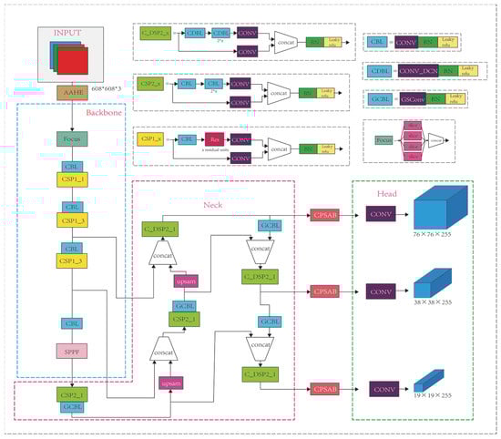
Figure 1.
Schematic diagram of RYOLOv5_D’s structure.
The RYOLOv5_D model consists of four main components: the input part, the backbone, the neck, and the head. The input part employs mosaic data augmentation and adaptive anchor boxes to adapt to the vehicle scene, enhancing the model’s robustness. Before entering the backbone, the AAHE algorithm is applied to enhance infrared images, followed by the focus module’s slice operation, which increases the channel numbers to obtain a feature map with twice the downsampling without losing information. The model’s backbone adopts the CSPDarknet53 structure, and the neck includes the FPN for transmitting high-level semantic features from the top to the bottom and the PAN for transmitting low-level localization features from the bottom to the top. The combination of FPN and PAN integrates semantic and localization features. The SPP module performs feature extraction and encoding on the image at four scales, and the C3 module incorporates the DCNv2 module, introducing learnable offset values in the receptive field to closely match the actual shape of the objects and cover the surrounding areas. This addresses the issue of excessively large aspect ratios for some vehicles in remote sensing effectively. The lightweight convolution GSconv module, constructed by mixing SC, DWC, and shuffle, replaces traditional CNN structures, reducing model parameters without additional operations and achieving noticeable accuracy gains. Three CPSAB attention modules are added between the neck and the output end, maintaining high resolution and computational efficiency while effectively connecting global information to obtain the detection results. The output end produces three different-scale M × M (19 × 19, 38 × 38, 76 × 76) outputs. Finally, the three feature layers of different scales are concatenated, resulting in a detection head capable of detecting objects of large, medium, and small scales.
RYOLOv5_D utilizes MetaAconC as an activation function. The backbone of RYOLOv5_D, CSPDarknet53, loads pre-trained weights trained on the standard COCO dataset. The model employs the circular smooth label (CLS) method [30] for circular smooth label encoding. This method utilizes labels with periodic circular encoding, transforming the continuous regression problem of angle prediction into a discrete classification problem.
3.1.2. Loss Function
The total loss is defined as the sum of four individual losses,
, , and , where each term corresponds to the angle loss, bounding box loss, confidence loss, and classification loss, respectively.
- Angle Loss:
Here, the input image is segmented into M×M cells, and each cell generates B-predicted bounding boxes. It is necessary to traverse through M×M×B candidate boxes of output cells. represents that the object in the i-th cell has the j-th candidate box as a positive sample. is the ground truth of the predicted angle. Binary cross-entropy is used to obtain the loss for the angle.
- Boundary Box Loss: Employ complete IoU (CIoU) to calculate the boundary box loss, incorporating the overlap area, center point distance, and aspect ratio simultaneously in the computation to enhance training stability and convergence speed.
Here, () represents the ground truth of (). c are the similarity of the diagonal length and aspect ratio of the minimum surround rectangle of boxes A and B, respectively. and are the areas of boxes A and B; is the influence factor; is the weight parameter. is the intersection of the two boxes, and the larger the IoU, the greater the effect on .
- Confidence Loss:
is the confidence degree of the prediction box, and is the ground truth of . represents the fact that the object is a positive sample in i cells.
- Classification Loss: Considering that a target may belong to multiple categories, a binary cross-entropy loss is used to treat each category.
represents the current predicted value for the category; represents the sigmoid-transformed probability for the category, and is the ground truth for the category .
3.2. Data Pre-Processing
First, select the images of four vehicle classes (car, truck, bus, and freight car) from the DroneVehicle dataset [31] and the VEDAI dataset [32]. Then, operations such as filtering, skewing, rotating, scaling, translating, mirroring, etc., are performed on the selected images (mixed transformations if necessary). Priority is given to images containing a higher proportion of small-sample vehicles to increase the proportion of small-sample vehicles while suppressing the proportion of large-sample vehicles, achieving data-balancing effects and reducing the severe overfitting caused by the “long-tail” distribution of the data. Since the transformations preserve straight lines on the images before and after the operation and maintain a balanced relationship, these operations can be equivalently considered to be affine transformations, which could expressed by the following formula:
A is the affine transformation matrix; (x, y, 1) represents the original pixel coordinates, and (, , 1) represents the pixel coordinates after the affine transformation. In the specific image processing procedure, the rotation angle is arbitrary; the skew angle is assumed to be (0°, 45°) by default, and the scaling factors are assumed to be (0.7, 1.3) by default. Figure 2 illustrates the sample image after having undergone the pre-processing steps.
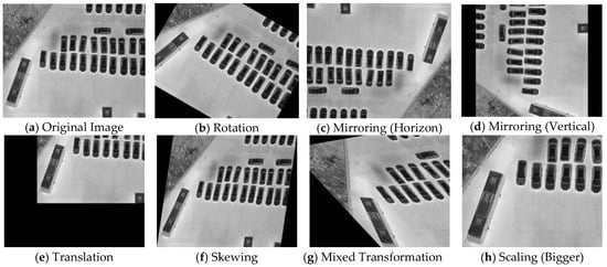
Figure 2.
Effect images after different affine transformations.
After undergoing skewing, flipping, cropping, scaling, and other affine transformations, the dataset was reannotated to create a new self-built dataset named BalancedVehicle. Due to the overwhelming quantity of cars, forcibly undersampling may lead to inefficient data utilization and the high cost of manual annotation. Therefore, the image pre-processing in the above figure is carried out to some extent to improve the composition of the images, without forcefully reducing the absolute balance of certain vehicle classes. Figure 3 illustrates the comparison of the vehicles’ distribution in different datasets.
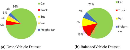
Figure 3.
Comparison of Infrared Vehicle Distribution.
3.3. Data Augmentation for Infrared Images
An infrared image can be considered as a superposition of target and background , as shown in the following equation:
This paper employs the automatic adaptive histogram equalization (AAHE) method during the image loading process to enhance infrared images. By computing the local maxima and minima adaptively as dynamic upper and lower bounds, the original image is equalized. This approach highlights vehicle targets while suppressing complex background information. Applying data augmentation AAHE methods during the model’s data loading stage in training helps one mitigate the issue of insufficient model training caused by various complex urban and road environments in infrared images. The AAHE algorithm is shown in Algorithm 1.
| Algorithm 1. Implementation steps of the AAHE algorithm. | |
| 1: | Input: Original image {(img1),(img2), ....., (imgN)}, Grayscale M, R=Q=([0.,0.,...])M*1 |
| 2: | Output: Enhanced image {(img1′), (img2′), (img3′), ....., (imgN’)} |
| 3: | Begin: |
| 4: | For img(x) in [1,N] do |
| 5: | Im_h,Im_w ← img(x).shape [0], img(x).shape[1] |
| 6: | For j in [1,Im_h] do |
| 7: | For k in [1,Im_w] do |
| 8: | R[img(i,j)] ← R[img(i,j)]+1, End For |
| 9: | N ← R[R>0], M ← N.shape, Max_sum = Min_sum = Max=Min ← 0, End for |
| 10: | For k in [0,N-2] do |
| 11: | Obtain local maxima and statistical maxima If (N[k+1] > N[k+2]) &(N[k+1] > N[i]) then |
| 12: | Max_sum ← Max_sum + N[k+1], Max ← Max + 1 |
| 13: | Obtain local minimum values and count the number of minimum values If (N[k+1] <N[k+2]) &(N[k+1] < N[k]) then |
| 14: | Min_sum ← Min_sum + N[k+1], Min ← Min + 1 |
| 15: | up_boundary ← Max_sum/Max, down_boundary ← Min_sum/Min, End for |
| 16: | For m in [1,M] do |
| 17: | If R[m] > up_boundary then Q[m] ← Q[m] + Up_boundary |
| 18: | else down_boundary < R[m] < Up_boundary then Q[m] ← Q[m] + R[m] |
| 19: | else R[m] <down_boundary then Q[m] ← Q[m] + down_boundary, End for |
| 20: | For i in [1,Im_h] do |
| 21: | For j in [1,Im_w] do |
| 22: | Obtain a new histogram of the gray-scale distribution Q[i, j] ← 255 * R[img(i,j)]/Q[m], End for, End for |
| 23: | End for |
To quantify the enhancement effect of AAHE on the infrared images, entropy (EN), standard deviation (SD) and spatial frequency (SF) are selected as objective evaluation indicators. One hundred images are randomly selected, and the arithmetic mean of each indicator is calculated before and after enhancement. The results of each indicator before and after enhancement are presented in Table 1. Larger values of information entropy, contrast, and spatial frequency indicate clearer edges and finer details of the image’s target. It is evident in Figure 4 that the contours of the vehicles are more distinct and that the overall image has a clearer sense of hierarchy. The formulas for EN, SD, and SF are defined as follows:

Table 1.
Comparison of index results after infrared image enhancement.
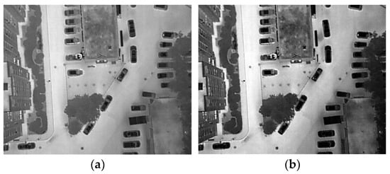
Figure 4.
Comparison of enhanced effects: (a) original image and (b) infrared augmented image.
represents 256 gray levels; represents the i-th gray level; represents the probability of the i-th gray level; W and H are the length and width of the image; represents the mean value of all the gray levels in the image, and represents the grayscale values below and to the left of the position (i, j).
3.4. Deformable Convolution Network (DCN)
The deformable convolution operation can flexibly extract information from different types of input images. This information can be understood as image features, which are manifested by each pixel in the image through a combination or an independent manner. Examples include texture features and color features in images. DCNv1 is shown in Figure 5. The formula for deformable convolution DCNv1 [33] is as follows:
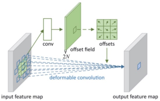
Figure 5.
Deformable convolution v1 diagram.
is the coordinate position of the center of the convolution core; is the relative position of the center of the convolution core; R = {(−1, −1), (−1, 0),..., (0, 1), (1, 1)}; w is the coordinate point weight, and is the learned floating-point data value.
The deformable convolution v1 (DCNv1) does not expand the convolutional kernel, actually; instead, it reorganizes the pixels in the input image before convolution. It obtains coordinate values with offset values after each convolution, effectively achieving the expansion of the convolutional kernel. This offset value is based on coordinate pixel points and needs to be obtained through bilinear interpolation to correspond to the image coordinates. This new feature map with a coordinate offset will be output as the input for the next layer. A convolution with offsets can better conform to the shape and size of complex objects, adapting to the demands of large aspect ratios and multi-scale object detection without requiring additional supervised learning. The formula for deformable convolution v2 (DCNv2) [13] is as follows:
In this article, we use DCNv2 to strengthen our model. DCNv2, built upon DCNv1, introduces weight coefficients in the range [0, 1]. These coefficients increase the weight information for each sampled point’s offset, assigning weights based on their relevance to the contextual semantic information of the sampled point. The modulated deformable convolution has a total of 3k offset channels, where 2k corresponds to learned biases and 1k corresponds to modulated biases, both of which are separated. This weight allocation mechanism allows for more accurate feature extraction. Additionally, DCNv2 can enhance the precision of offset correction by stacking multiple blocks, providing stronger spatial transformation capabilities. Figure 6 compares the addition of DCNv2 heatmaps in the neck part of the model. It is evident that the model’s perception of vehicle targets has been improved, with the region of interest closer to the area where vehicles are located. The model also pays more attention to vehicles with larger aspect ratios, resulting in improved accuracy compared to the baseline.
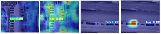
Figure 6.
Heatmap comparison after adding deformable module DCN v2.
3.5. Convolutional Polarized Self-Attention Block (CPSAB)
We propose a novel attention module in this paper called CPSAB based on the polarized self-attention block (PSA) [14]. PSA is a refined dual-attention mechanism that operates on the input tensor X to highlight or suppress features, similar to the filtering of light through an optical lens, hence the name “polarized filtering”. PSA excels in both channel and spatial dimensions without significant compression. It maintains dimensions of C/2 on the channel component and [H, W] on the spatial component, reducing the information loss caused by the dimension reduction. The convolutional polarized self-attention block (CPSAB) extends the PSA mechanism by adding average and max pooling modules to it. This makes the information better integrated. We then use a SC with a kernel of size 7 to connect them. The structure of the CPSAB module is illustrated in Figure 7. The spatial-wise self-attention in the CPSAB module employs a 1 × 1 convolution to transform the input features into two parts, denoted as and . For the features, the channel dimension is compressed to 1, while the channel dimension of the features is maintained at C/2. Subsequently, softmax information enhancement is applied to the features, and the matrix multiplication of and yields C. This result undergoes a 1 × 1 convolution operation, followed by layer normalization, increasing the channel number to C, and, finally, is normalized through a sigmoid for the ease of subsequent operations. Channel-wise attention is similar to the spatial-wise attention steps. The final obtained w features, due to the two independently operated steps in the channel and spatial dimensions, cannot truly achieve the fusion of the channel and spatial information. To address this, the obtained w features undergo an average pooling module and a max pooling module. Subsequently, SC operations are applied to enhance the correlation between the channel and spatial features, resulting in the generation of a final uniformly blended feature.
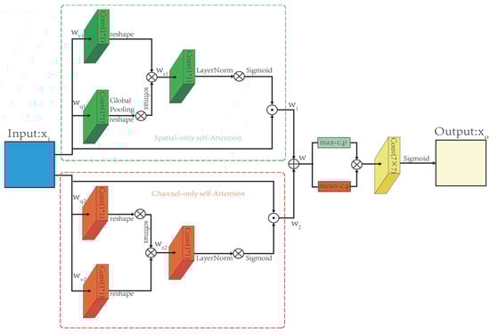
Figure 7.
Structure of the CPSAB module. Conv (7 × 7) represents a convolution with kernel size 7.
Among them, ; represents the sigmoid function; represents the softmax operation; represents the sigmoid operation; “” represents the convolution operation; represents the multiplication operator; represents the global average pooling; represents the average pooling, and represents the max pooling.
3.6. Lightweight Module (GSConv)
The GSConv [15] module, commonly utilized in the visual systems of autonomous driving vehicles, enhances model accuracy while reducing model complexity, achieving a balance between precision and speed. Figure 8 illustrates the overall structure of GSConv. In the transfer process of CNN within the backbone, spatial information gradually propagates through the channels. However, each spatial compression and channel expansion of the feature map results in semantic loss. GSConv maximally preserves channel connections, which may be lost with DWConv. GSConv is primarily used in the neck part of the network, as excessive usage can increase inference time. In the GSConv structure, the input image undergoes standard convolution (SC) for the number of channels, followed by depth-wise separable convolution (DWConv) for the number of channels and concatenation. Channel shuffling is applied to enable mutual communication between the two convolutional feature channels, allowing information from the shuffle module to be fully integrated into the output of the DWConv. This strategy ensures the even exchange of local feature information between different channels. Importantly, it avoids introducing additional model computational overhead, and the time complexity remains only .
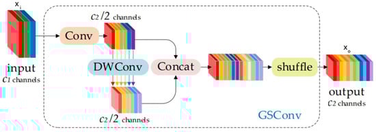
Figure 8.
Structure of the GSConv. Different colors is used to distinguish between different layers.
4. Vehicle Object Detection Evaluation
The commonly used evaluation metrics for vehicle object detection can be roughly divided into three categories: model size evaluation metrics, model accuracy evaluation metrics, and model real-time evaluation metrics.
4.1. Model Size Evaluation Metrics
Model size evaluation metrics primarily include parameters (Param).
Param refers to the total number of parameters that need to be trained during model training and is used to measure the model’s size (i.e., compute space complexity).
4.2. Model Size Evaluation Metrics
Model accuracy evaluation metrics include the following: precision, recall, average precision (AP), F1, and mean average precision (mAP).
Precision represents the proportion of correctly identified positive samples to the total number of predicted positive samples, while recall indicates the proportion of correctly identified positive samples in the total number of actual positive samples. Precision and recall often involve trade-offs; as precision increases, recall may decrease and vice versa. When evaluating model performance, both precision and recall need to be considered simultaneously. The calculation formulas are as follows:
True positives () are predicted as positive and are actually positive; false positives () are predicted as positive but are actually negative; false negatives () are predicted as negative but are actually positive. True negatives (TN) are predicted as negative but are actually positive.
The PR curve is plotted with precision on the y-axis and recall on the x-axis. The higher the precision and recall of the model, the better its performance, corresponding to a larger area under the PR curve. The area under the PR curve, denoted as AUC-PR, is defined as the integral of the PR curve. A larger AUC-PR indicates a higher average precision of the model. As shown in Figure 9 below, the PR test curves are presented.
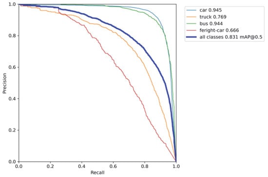
Figure 9.
PR curve.
F1 is the harmonic mean of precision and recall, with a range of (0, 1). When precision (P) and recall (R) approach 1, the F1 score also approaches 1, indicating better model performance. The formula for this calculation is as follows:
refers to the mean precision across different types of object detection accuracies. In the detection of multiple object classes, is calculated for each individual category and then is computed by averaging all the values. serves as a comprehensive measure of the average accuracy of the detected targets, where represents the number of categories of targets in the dataset. The calculation formula is as follows:
4.3. Model Real-Time Performance Metrics
The evaluation metrics for the model real-time performance include frames per second (FPS) and giga floating-point operations per second (GFLOPS):
FPS is the number of image frames processed per second. A higher frame rate results in smoother motion. Typically, a minimum of 30 frames per second is required to avoid choppy motion. FPS is used to measure the speed of the model.
GFLOPS is the number of floating-point operations per second, measured in billions giga. It can be understood as the computational complexity of the model, representing the algorithm’s complexity. GFLOPS is commonly used to assess the computational load of an algorithm.
5. Experiment
5.1. Experimental Configuration
Table 2 provides detailed information about the hardware, software platforms, and dataset used in our experimental environment, while Table 3 outlines the parameters configured during the experimental process.
Table 2.
Configurations.
Table 3.
Experimental parameter settings.
The input image size is based on the standard size of the dataset. For the BalancedVehicle dataset, the standard size is 820 × 712 pixels, and the output size is set to be the same as the input image size. The training is configured with a maximum of 300 epochs, although the model typically converges around 120 epochs, and the accuracy tends to exhibit minor fluctuations beyond that point.
5.2. Related Dataset
5.2.1. DroneVehicle Dataset
The DroneVehicle dataset is created by Tianjin University. As is shown in Figure 10, the DroneVehicle dataset is a large RGB-T remote sensing vehicle dataset captured by unmanned aerial vehicles (UAVs). The dataset comprises a total of 56,878 aerial images, with 452,570 visible light vehicle targets and 500,517 infrared vehicle targets, totaling 953,087 annotated vehicle targets. The higher count of infrared targets compared to visible light targets is due to the dataset covering various times of the day, including daytime, evening, and nighttime, capturing complex road information. The images were taken at different angles (15°, 30°, 45°) and heights (80 m, 100 m, 120 m), featuring diverse environments such as highways, streets, parking lots, and other scenarios.
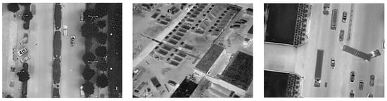
Figure 10.
DroneVehicle partial image display.
5.2.2. VEDAI Dataset
The VEDAI dataset is designed for multi-class vehicle detection in aerial images and was captured using the HRO 2012 6-inch kit. The VEDAI dataset is shown in Figure 11. It consists of 3708 objects across the following nine categories: boat, car, camping car, plane, van, tractor, truck, freight car, and others. The dataset’s images were collected during the spring of 2012, with each image having two color images, including an RGB color image and a near-infrared (NIR) image. The dataset contains a total of 2538 aerial remote sensing images at two different scales (1024 × 1024 and 512 × 512) from the Utah AGRC. There are 1210 images each for infrared and visible light remote sensing, with a spatial resolution of 12.5 cm. The dataset includes annotations for the center point and orientation of the objects, and it also indicates whether an object is occluded.
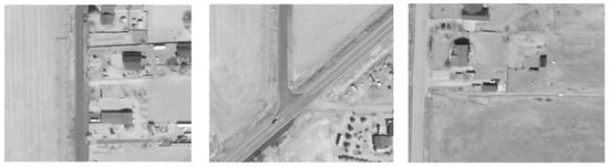
Figure 11.
VEDAI partial image display.
5.2.3. BalancedVehicle Self-Built Dataset
By selecting images from the DroneVehicle dataset and a small portion of the VEDAI dataset as the data samples, various affine transformations are applied to balance the dataset. The dataset comprises a total of 3000 aerial images, featuring the following four vehicle categories: cars, trucks, buses, and freight cars. The dataset was split into training (2132 images), validation (850 images), and testing (288 images) sets in a ratio of 7:2:1. Table 4 shows the distribution of various vehicles. It includes diverse road scenarios captured at different times of the day, including daytime, dusk, and nighttime, as well as complex road information captured at various shooting heights and angles.
Table 4.
Distribution of various vehicle categories in the BalancedVehicle dataset.
5.3. Ablation Experiments
From Table 5, it is clear that the accuracy of YOLOv5s-obb for cars and buses is already high.; the added modules mainly enhance the accuracy for trucks and freight cars.
Table 5.
Results of the ablation experiments for comparison.
It is vividly shown in Table 5, using the AAHE algorithm, which highlights infrared vehicle targets while suppressing background interference, that the AP for trucks increases by 3.4% and that for freight cars increases by 3.2%, with no additional Param increases. Next, with the addition of the CSPAB module, the model can focus on key vehicle target areas, resulting in a 4.9% increase in AP for freight cars and a 5.7% increase for trucks. Furthermore, by adding the DCNv2, which enlarges the receptive field and enhances the geometric transformation ability of the convolution, a better fitting of vehicle targets is achieved. The AP for trucks and freight cars, which have large aspect ratios, increases by 9.1% and 5.1%, respectively, demonstrating that deformable convolution can adapt to challenging vehicle targets and improve detection accuracy. Finally, to meet real-time detection requirements and achieve a superior accuracy, the GSConv module is added. This addition operation reduces Param by 1.29M. With an increase of only 0.23M in the Param compared to the original YOLOv5s-obb and increases of 11.4% and 8% in the AP for trucks and freight cars, respectively, the mAP and mAP0.5:0.95 increase by 4.9% and 5.5%. From Table 6, it is evident that, with increasing depth, the RYOLOv5_D models show improved accuracy, making them suitable for real-time detection needs. Figure 12 visually demonstrates that the modified RYOLOv5s_D model enhances detection performance in challenging scenarios. Figure 13 depicts four loss curves during the training process.
Table 6.
Scores for different depths of RYOLOv5s_D models on Param, GFLOPS, FPS, mAP, and F1. The FPS and GFLOPS are measured during inference with a fully loaded 3080Ti, using an input image size of (840, 712).
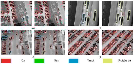
Figure 12.
Detection performance comparison between YOLOv5s-obb and RYOLOv5s_D. The subfigures (a) show scenes with complex backgrounds, (b) depict situations with large vehicle aspect ratios, (c) demonstrate scenarios with densely distributed and rotated vehicles, and (d) present drones captured from different angles.
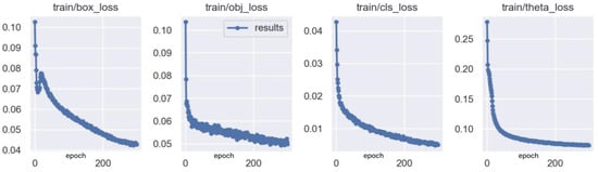
Figure 13.
Loss function curves during the training phase of the model.
5.4. Comparison of Detection Performance on the BalancedVehicle Dataset
Figure 14 shows the detection results of nine different advanced algorithms, including (c) CFA, (d) Faster R-CNN-O, (e) FCOS, (f) Gliding vertex, (g) Oriented RepPoints, (h) R3Det, (i) R-CNN-O, (j) Roi Transformer, and the proposed (k) RYOLOv5l_D, in the following four challenging scenarios: ① complex background, ② intensively distributed and rotated vehicles, ③ detection of vehicles with large aspect ratios, and ④ drones captured from different angles. In the detection results of scenario ①, it can be observed that most algorithms can detect vehicles even when they are partially obscured by trees on the left side. However, when four or five vehicles are closely arranged, it becomes easier to lose targets. Roi Transformer, Gliding vertex, and RYOLOv5l_D adapt better to this occluded environment than the other algorithms. In the detection results of scenario ②, all the algorithms perform well when vehicles are continuously clustered. However, if a single vehicle appears in the middle of the clustered vehicles, FCOS fails to detect the two vehicles in the middle and CFA, R3Det, and Roi Transformer mistakenly detect these two vehicles as trucks. RYOLOv5l_D exhibits some instances of duplicate bounding boxes. In the detection results of scenario ③, Oriented RepPoints and FCOS show poor detection performances, especially in missing truck detections. Gliding vertex’s bounding boxes do not tightly fit the vehicle bodies, resulting in suboptimal detection. Faster R-CNN-O, Roi Transformer, R-CNN-O, and R3Det exhibit false positives, misclassifying trucks as freight cars. RYOLOv5l_D achieves good detection results but may have instances of duplicate bounding boxes. In the detection results of scenario ④, RYOLOv5l_D can accurately frame closely arranged vehicles. Other algorithms encounter significant issues with both false negatives and false positives when dealing with such densely arranged vehicles captured from different angles.
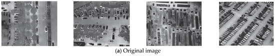
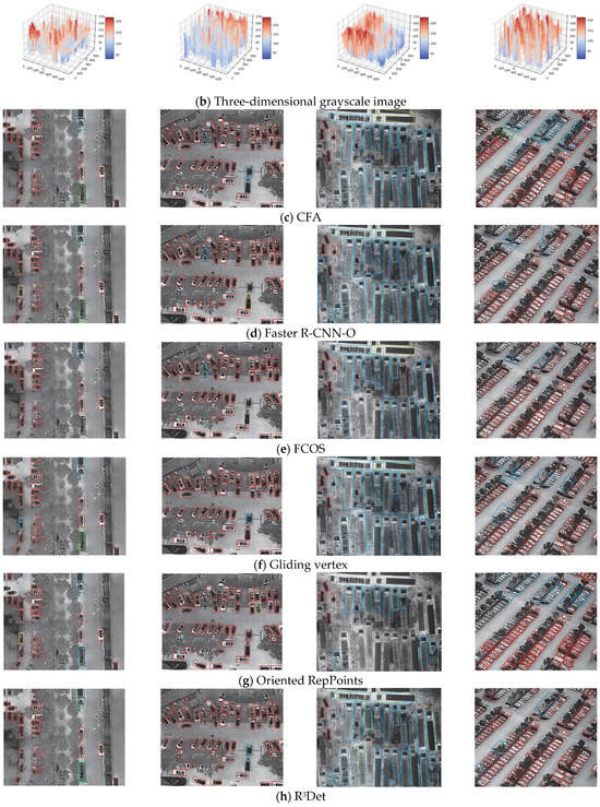
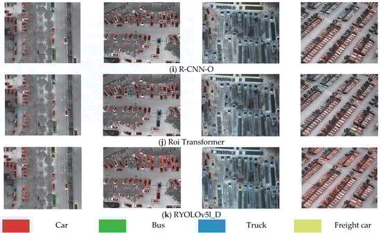
Figure 14.
Comparison of detection performance in four challenging scenarios for nine advanced object detection algorithms.
5.5. Experimental Comparison of Different Models on the BalancedVehicle Dataset
During training, the default input image size is set to 840 × 712 pixels. Multi-scale training and testing methods are not used in this experimental process. Table 7 displays the result of different network methods. GFLOPS and Param represent the model’s inference speed and the model’s scale, respectively. “+” indicates modifications to the model’s depth in order to distinguish it from the original model.
Table 7.
Result of different network methods on the BalancedVehicle dataset (rotated bounding boxes).
The experimental results reveal that RYOLOv5_D, RTMDet, and YOLOv5s-obb outperform the other algorithms in detecting infrared remote sensing vehicle targets. Among them, RYOLOv5l_D exhibits the best detection performance for the car and bus vehicle categories, achieving high levels of accuracy for the truck and freight car categories as well. The accuracy of the RYOLOv5_D series’ algorithms surpasses that of most algorithms, especially as the model depth increases. They have advantages in both accuracy and computational complexity, making them well-suited for various detection tasks involving infrared images in complex urban and road backgrounds with large vehicle aspect ratios and varying shooting angles. RYOLOv5s_D, with an input image size of 840 × 712, has a Param of only 7.87 M, second only to YOLOv5s-obb. Its Param corresponds to 10% of the RoI Transformer+’s Param and 13% of the Faster R-CNN-O’s Param. The model’s computational load is only 16.8 GFLOPS, which is 49.7% of the lightweight ReDet model’s load. Moreover, RYOLOv5l_D achieves an accuracy of 84.3%, with a Param of 4.56 M less than that of RTMDet-L. The model’s computational load is also 24.9 GFLOPS less than that of RTMDet-L, striking a balance between high accuracy and speed, making it highly practical for deployment. In the end, RYOLOv5m_D and RYOLOv5l_D only increase the Param count from that of the original model by 0.87 M and 1.6 M, respectively, with decreases in computational complexity of 4.5 GFLOPS and 12.8 GFLOPS.
6. Conclusions
This paper presents a novel infrared vehicle remote sensing target detection algorithm, RYOLOv5_D, designed to address various challenges encountered in the processing of infrared remote sensing images, such as complex backgrounds, large vehicle aspect ratios, disproportionate representation of single vehicle classes, and varying shooting angles. Initially, a self-built image dataset, BalancedVehicle, is introduced to mitigate the issue of overfitting caused by imbalanced class proportions. Subsequently, prior to model loading, the infrared image enhancement algorithm AAHE is employed for data pre-processing to reduce the interference of complex background information and enable thorough model training. Building upon this foundation, DCNv2 is utilized to enhance the detection accuracy of challenging vehicles with large aspect ratios, and the CPSAB module is incorporated to further improve the detection performance on difficult-to-detect vehicle targets. Finally, the GSConv module is introduced to reduce the model’s Param while enhancing accuracy. Compared to the YOLOv5-obb model, RYOLOv5s_D only increases the Param by 0.23M and improves mAP by 4.9%, specifically achieving notable improvements in the AP for trucks and freight cars of 11.4% and 8%, respectively. RYOLOv5m_D and RYOLOv5l_D exhibit impressive mAP accuracies of 82.6% and 84.3%, respectively, surpassing the accuracy of most detection algorithms. Regarding detection speeds, RYOLOv5s_D, RYOLOv5m_D, and RYOLOv5l_D achieve frame rates of 59.52, 44.64, and 29.58 FPS, respectively, meeting real-time vehicle detection requirements.
Despite the high accuracy and speed of RYOLOv5_D, there are limitations, including the occurrence of noticeable overlapping boxes, making visual observations challenging. Additionally, the model only utilizes infrared single-source images for object detection. We aim to explore the following in future works: ① We prepare to incorporate fusion with visible light images to complement information from both sources and achieve better practical detection results. ② We notice that zero-shot detection (ZSD) models can categorize new unseen instances of data. If ZSD models were used for vehicle detection, they could expand the fine granularity of vehicle detection. However, our RYOLOv5_D model may have a higher accuracy because it is based on a supervised method. ③This paper uses the pre-trained weights of the COCO dataset to train the model. However, if the BigDetection dataset with a larger data volume and more variety was used for pre-training, we believe that we could better initialize the weight of the dataset and speed-up its training efficiency. ④ Given the rapid development of large language models (LLMs), adding LLMs to the detector could strengthen the model’s real-time detection capability with appropriate parsing and post processing.
Author Contributions
Conceptualization, X.J. and F.W.; methodology, C.Y., F.W. and Y.F.; software, C.Y., Y.F. and X.L.; validation, C.Y., Y.Z., T.F. and J.P.; formal analysis, C.Y. and F.W.; resources, X.J.; data curation, C.Y. and X.L.; writing—original draft preparation, C.Y. and X.J.; writing—review and editing, C.Y. and F.W.; project administration, X.J., Y.F. and T.F.; funding acquisition, X.J. and F.W. All authors have read and agreed to the published version of the manuscript.
Funding
This research was funded by the National Key R&D Program of China, with grant number 2022YFB3902300, and was funded by the National Natural Science Foundation of China, with grant number 42001345.
Informed Consent Statement
Not applicable.
Data Availability Statement
The data and fundamental coding principles of this research are available at https://github.com/hukaixuan19970627/yolov5_obb (accessed on 7 January 2022) and https://github.com/VisDrone/DroneVehicle (accessed on 29 December 2021).
Conflicts of Interest
The authors declare no conflicts of interest.
References
- Vollmer, M. Infrared. Eur. J. Phys. 2013, 34, S49. [Google Scholar] [CrossRef][Green Version]
- Ajakwe, S.O.; Ihekoronye, V.U.; Akter, R.; Kim, D.-S.; Lee, J.M. Adaptive Drone Identification and Neutralization Scheme for Real-Time Military Tactical Operations. In Proceedings of the 2022 International Conference on Information Networking (ICOIN), Jeju-si, Republic of Korea, 12–15 January 2022; pp. 380–384. [Google Scholar]
- Mo, N.; Yan, L. Improved Faster RCNN Based on Feature Amplification and Oversampling Data Augmentation for Oriented Vehicle Detection in Aerial Images. Remote Sens. 2020, 12, 2558. [Google Scholar] [CrossRef]
- Wang, B.; Gu, Y. An Improved FBPN-Based Detection Network for Vehicles in Aerial Images. Sensors 2020, 20, 4709. [Google Scholar] [CrossRef]
- Deng, Z.; Sun, H.; Zhou, S.; Zhao, J.; Zou, H. Toward Fast and Accurate Vehicle Detection in Aerial Images Using Coupled Region-Based Convolutional Neural Networks. IEEE J. Sel. Topics Appl. Earth Observ. Remote Sens. 2017, 10, 3652–3664. [Google Scholar] [CrossRef]
- Wang, H.; Wang, Q.; Yang, F.; Zhang, W.; Zuo, W. Data Augmentation for Object Detection via Progressive and Selective Instance-Switching. arXiv 2019, arXiv:1906.00358. [Google Scholar]
- Zhong, J.; Lei, T.; Yao, G. Robust Vehicle Detection in Aerial Images Based on Cascaded Convolutional Neural Networks. Sensors 2017, 17, 2720. [Google Scholar] [CrossRef] [PubMed]
- Shen, J.; Liu, N.; Sun, H.; Tao, X.; Li, Q. Vehicle Detection in Aerial Images Based on Hyper Feature Map in Deep Convolutional Network. KSII Trans. Internet Inf. Syst. (TIIS) 2019, 13, 1989–2011. [Google Scholar]
- Musunuri, Y.R.; Kwon, O.-S.; Kung, S.-Y. SRODNet: Object Detection Network Based on Super Resolution for Autonomous Vehicles. Remote Sens. 2022, 14, 6270. [Google Scholar] [CrossRef]
- Li, J.; Zhang, Z.; Tian, Y.; Xu, Y.; Wen, Y.; Wang, S. Target-Guided Feature Super-Resolution for Vehicle Detection in Remote Sensing Images. IEEE Geosci. Remote Sens. Lett. 2021, 19, 1–5. [Google Scholar] [CrossRef]
- Mostofa, M.; Ferdous, S.N.; Riggan, B.S.; Nasrabadi, N.M. Joint-SRVDNet: Joint Super Resolution and Vehicle Detection Network. IEEE Access 2020, 8, 82306–82319. [Google Scholar] [CrossRef]
- Wan, M.; Gu, G.; Qian, W.; Ren, K.; Chen, Q.; Maldague, X. Infrared Image Enhancement Using Adaptive Histogram Partition and Brightness Correction. Remote Sens. 2018, 10, 682. [Google Scholar] [CrossRef]
- Zhu, X.; Hu, H.; Lin, S.; Dai, J. Deformable Convnets v2: More Deformable, Better Results. In Proceedings of the 2019 IEEE/CVF Conference on Computer Vision and Pattern Recognition (CVPR), Long Beach, CA, USA, 15–20 June 2019; pp. 9308–9316. [Google Scholar]
- Liu, H.; Liu, F.; Fan, X.; Huang, D. Polarized Self-Attention: Towards High-Quality Pixel-Wise Regression. arXiv 2021, arXiv:2107.00782. [Google Scholar]
- Li, H.; Li, J.; Wei, H.; Liu, Z.; Zhan, Z.; Ren, Q. Slim-Neck by GSConv: A Better Design Paradigm of Detector Architectures for Autonomous Vehicles. arXiv 2022, arXiv:2206.02424. [Google Scholar]
- Mateus, B.C.; Mendes, M.; Farinha, J.T.; Cardoso, A.J.M.; Assis, R.; da Costa, L.M. Forecasting Steel Production in the World—Assessments Based on Shallow and Deep Neural Networks. Appl. Sci. 2022, 13, 178. [Google Scholar] [CrossRef]
- Wei, H.; Zhang, Y.; Chang, Z.; Li, H.; Wang, H.; Sun, X. Oriented Objects as Pairs of Middle Lines. ISPRS J. Photogramm. Remote Sens. 2020, 169, 268–279. [Google Scholar] [CrossRef]
- Lin, Y.; Feng, P.; Guan, J.; Wang, W.; Chambers, J. IENet: Interacting Embranchment One Stage Anchor Free Detector for Orientation Aerial Object Detection. arXiv 2019, arXiv:1912.00969. [Google Scholar]
- Lyu, C.; Zhang, W.; Huang, H.; Zhou, Y.; Wang, Y.; Liu, Y.; Zhang, S.; Chen, K. Rtmdet: An Empirical Study of Designing Real-Time Object Detectors. arXiv 2022, arXiv:2212.07784. [Google Scholar]
- Yang, X.; Yan, J.; Feng, Z.; He, T. R3det: Refined Single-Stage Detector with Feature Refinement for Rotating Object. In Proceedings of the AAAI Conference on Artificial Intelligence, Virtually, 2–9 February 2021; Volume 35, pp. 3163–3171. [Google Scholar]
- Han, J.; Ding, J.; Li, J.; Xia, G.-S. Align Deep Features for Oriented Object Detection. IEEE Trans. Geosci. Remote Sens. 2021, 60, 1–11. [Google Scholar] [CrossRef]
- Liu, Z.; Hu, J.; Weng, L.; Yang, Y. Rotated Region Based CNN for Ship Detection. In Proceedings of the 2017 IEEE International Conference on Image Processing (ICIP), Beijing, China, 17–20 September 2017; pp. 900–904. [Google Scholar]
- Jiang, Y.; Zhu, X.; Wang, X.; Yang, S.; Li, W.; Wang, H.; Fu, P.; Luo, Z. R2CNN: Rotational Region CNN for Orientation Robust Scene Text Detection. arXiv 2017, arXiv:1706.09579. [Google Scholar]
- Nabati, R.; Qi, H. Rrpn: Radar Region Proposal Network for Object Detection in Autonomous Vehicles. In Proceedings of the 2019 IEEE International Conference on Image Processing (ICIP), Taipei, Taiwan, 22–25 September 2019; pp. 3093–3097. [Google Scholar]
- Ding, J.; Xue, N.; Long, Y.; Xia, G.-S.; Lu, Q. Learning RoI Transformer for Oriented Object Detection in Aerial Images. In Proceedings of the 2019 IEEE/CVF Conference on Computer Vision and Pattern Recognition (CVPR), Long Beach, CA, USA, 15–20 June 2019; pp. 2849–2858. [Google Scholar]
- Li, X.; Cai, Z.; Zhao, X. Oriented-YOLOv5: A Real-Time Oriented Detector Based on YOLOv5. In Proceedings of the 2022 7th International Conference on Computer and Communication Systems (ICCCS), Wuhan, China, 22–25 April 2022; pp. 216–222. [Google Scholar]
- Zhao, X.; Xia, Y.; Zhang, W.; Zheng, C.; Zhang, Z. YOLO-ViT-Based Method for Unmanned Aerial Vehicle Infrared Vehicle Target Detection. Remote Sens. 2023, 15, 3778. [Google Scholar] [CrossRef]
- Mehta, S.; Rastegari, M. Mobilevit: Light-Weight, General-Purpose and Mobile-Friendly Vision Transformer. arXiv 2021, arXiv:2110.02178. [Google Scholar]
- Bao, C.; Cao, J.; Hao, Q.; Cheng, Y.; Ning, Y.; Zhao, T. Dual-YOLO Architecture from Infrared and Visible Images for Object Detection. Sensors 2023, 23, 2934. [Google Scholar] [CrossRef]
- Yang, X.; Yan, J. Arbitrary-Oriented Object Detection with Circular Smooth Label; Springer: Berlin/Heidelberg, Germany, 2020; pp. 677–694. [Google Scholar]
- Sun, Y.; Cao, B.; Zhu, P.; Hu, Q. Drone-Based RGB-Infrared Cross-Modality Vehicle Detection via Uncertainty-Aware Learning. IEEE Trans. Circuits Syst. Video Technol. 2022, 32, 6700–6713. [Google Scholar] [CrossRef]
- Razakarivony, S.; Jurie, F. Vehicle Detection in Aerial Imagery: A Small Target Detection Benchmark. J. Visual Commun. Image Represent. 2016, 34, 187–203. [Google Scholar] [CrossRef]
- Dai, J.; Qi, H.; Xiong, Y.; Li, Y.; Zhang, G.; Hu, H.; Wei, Y. Deformable Convolutional Networks. In Proceedings of the 2017 IEEE International Conference on Computer Vision (ICCV), Venice, Italy, 22–29 October 2017; pp. 764–773. [Google Scholar]
- Lee, S.; Lee, S.; Song, B.C. Cfa: Coupled-Hypersphere-Based Feature Adaptation for Target-Oriented Anomaly Localization. IEEE Access 2022, 10, 78446–78454. [Google Scholar] [CrossRef]
- Li, Z.; Hou, B.; Wu, Z.; Ren, B.; Yang, C. FCOSR: A Simple Anchor-Free Rotated Detector for Aerial Object Detection. Remote Sens. 2023, 15, 5499. [Google Scholar] [CrossRef]
- Li, W.; Chen, Y.; Hu, K.; Zhu, J. Oriented Reppoints for Aerial Object Detection. In Proceedings of the 2022 IEEE/CVF Conference on Computer Vision and Pattern Recognition (CVPR), New Orleans, LA, USA, 18–24 June 2022; pp. 1829–1838. [Google Scholar]
- Han, J.; Ding, J.; Xue, N.; Xia, G.-S. Redet: A Rotation-Equivariant Detector for Aerial Object Detection. In Proceedings of the 2021 IEEE/CVF Conference on Computer Vision and Pattern Recognition (CVPR), Nashville, TN, USA, 20–25 June 2021; pp. 2786–2795. [Google Scholar]


Disclaimer/Publisher’s Note: The statements, opinions and data contained in all publications are solely those of the individual author(s) and contributor(s) and not of MDPI and/or the editor(s). MDPI and/or the editor(s) disclaim responsibility for any injury to people or property resulting from any ideas, methods, instructions or products referred to in the content. |
© 2024 by the authors. Licensee MDPI, Basel, Switzerland. This article is an open access article distributed under the terms and conditions of the Creative Commons Attribution (CC BY) license (https://creativecommons.org/licenses/by/4.0/).