VID-SLAM: Robust Pose Estimation with RGBD-Inertial Input for Indoor Robotic Localization

Abstract

This study proposes a tightly coupled multi-sensor Simultaneous Localization and Mapping (SLAM) framework that integrates RGB-D and inertial measurements to achieve highly accurate 6 degree of freedom (6DOF) metric localization in a variety of environments. Through the consideration of geometric consistency, inertial measurement unit constraints, and visual re-projection errors, we present visual-inertial-depth odometry (called VIDO), an efficient state estimation back-end, to minimise the cascading losses of all factors. Existing visual-inertial odometers rely on visual feature-based constraints to eliminate the translational displacement and angular drift produced by Inertial Measurement Unit (IMU) noise. To mitigate these constraints, we introduce the iterative closest point error of adjacent frames and update the state vectors of observed frames through the minimisation of the estimation errors of all sensors. Moreover, the closed-loop module allows for further optimization of the global attitude map to correct the long-term drift. For experiments, we collect an RGBD-inertial data set for a comprehensive evaluation of VID-SLAM. The data set contains RGB-D image pairs, IMU measurements, and two types of ground truth data. The experimental results show that VID-SLAM achieves state-of-the-art positioning accuracy and outperforms mainstream vSLAM solutions, including ElasticFusion, ORB-SLAM2, and VINS-Mono.

1. Introduction and Related Work

Visual localization and dense 3D reconstruction are high-demand research areas, forming the core technology of a broad range of indoor and outdoor applications. Compared to using a single sensor, multiple sensor-based Simultaneous Localization and Mapping (SLAM) approaches are more robust, as the sensors can be used in a complementary manner for motion estimation. The emerging RGB-D cameras with integrated internal sensors (e.g., Intel Realsense) significantly reduce the hardware cost and have the potential to be widely applied in various scenarios.

SLAM is important for a broad range of applications, such as mobile robotics and Augmented Reality/Virtual Reality (AR/VR). Pursuing an affordable yet robust solution as a trade-off between complexity and accuracy is challenging. In recent years, pioneering research [1,2] using a combination of multiple sensors has achieved promising performance in large-scale localization [3,4]. For example, the use of a monocular SLAM system [5] can significantly reduce the hardware cost. However, monocular SLAM is sensitive to initialization, and the scale-drifting problem is hard to mitigate due to the unobservability of depth. To obtain the metric scale, researchers have proposed using a low-cost Inertial Measurement Unit (IMU) as a complement to monocular odometry to improve the motion tracking performance [6].

There are a variety of sensors that can achieve the state estimation required in the SLAM process, such as the IMU, RGB-D camera, monocular camera, and LiDAR. How to use low-cost sensors to achieve high-precision state estimation is a challenging exploration process. An IMU can provide measurements of the acceleration and angular velocity of the current object, but cannot directly be used to estimate its state. Moreover, the measurements provided by a cheap IMU are not accurate enough for localization, and residuals after IMU pre-integration are inevitable. Visual and inertial fusion makes low-cost state estimation possible. Visual constraints depend on the features of scenarios, and the quality of feature extraction determines whether the estimated depth is reliable. The Vision-Inertial System (VINS), one of the current state-of-the-art models in Vision-aided Inertial Odometry (VIO), is still greatly restricted in featureless scenes. The use of a depth-based odometer has achieved impressive effects in state estimation. The Iterative Closest Point (ICP) algorithm is accurate and fast for point set registration on the same scale, and has been widely used for pose estimation and establishing point correspondences. Note that depth-based systems often suffer from cumulative error, and some of these errors cannot be corrected by loop closure detection.

The IMU is an essential component of navigation, positioning, and motion control. However, IMU-based state estimation cannot avoid the occurrence of drift, including linear horizontal angular drift and exponential positional drift, which limits the use of single sensors. It is widely accepted that monocular SLAM suffers from problematic metric scale estimation. The fusion of visual data with IMU measurements provides a direct solution to this problem. The Multi-State Constraint Kalman Filter (MSCKF) [7] is a widely used Extended Kalman Filter (EKF) based on the Visual-Inertial Odometry (VIO) method. In this method, six degrees-of-freedom (6DOF) poses, comprising positions and quaternions, are used as state vectors instead of 3D feature positions. The geometric consistency of visual features appearing in multiple frames is used to update the state vector with multiple forms of constraints. However, this approach is not suitable for long-term operation due to the exponential growth of the state vector dimensions in the system, leading to a consequent increase in computational complexity. VINS-Mono [8] is a state-of-the-art VIO system requiring only a monocular camera and an IMU. This system achieves positioning performance comparable to Open Keyframe-Based Visual-Inertial SLAM (OKVIS) [9], and is more robust as a full SLAM system. VINS-Mono achieves real-time performance on mobile devices and is, to the best of our knowledge, the first optimization-based VIO that can be deployed on embedded platforms as well. When the camera moves in a straight line in a planar environment, its trajectory is at a constant velocity, resulting in near-zero acceleration. In this case, mainstream VIOs often lead to inaccurate estimates as they are affected by additional unobservable directions. In addition to the effects of IMU noise, high illumination variations and few features can pose additional challenges to the visual tracking process as well.

Notably, the use of available depth information has made significant progress in state estimation. As a seminal work, Kinectfusion [10], presented by Richard et al., is the first SLAM algorithm for real-time localization and 3D reconstruction using a moving depth camera. The ICP algorithm of Kinectfusion, which is foundational to this approach, traces back to the earlier work by Zhang et al. [11]. As the system only operates in small scenes (tens of meters) and does not include closed-loop detection, its application is limited to indoor environments. Building on this, an extended Kinectfusion framework, Kintinuous [12], was proposed much later to enhance scalability. This system updates the 3D model by rolling a circular buffer for more efficient spatial utilization and fuses ICP iterations with photometric constraints for camera pose tracking. Additionally, they integrated the Bags of Binary Words (DBoW) location recognition system [13] for closed-loop detection, enabling correction for long-term drift (e.g., several hundred meters).

Inspired by surfel-based fusion systems, Thomas et al. have proposed ElasticFusion [14], a map-centric approach. This system optimizes trajectories using both geometric and photometric constraints. Its reliance on active and inactive models within the same camera frame, which helps to maintain the map distribution, could potentially limit its adaptability in dynamic environments when compared to other SLAM systems. Mur-Artal et al. have introduced ORB-SLAM [15], a monocular vision-based SLAM approach with high localization accuracy. In their further development, ORB-SLAM2 [16], they included additional sensor combinations (stereo and RGB-D), thereby increasing the system’s versatility. The use of a co-visibility graph and the DBoW2 [17] library in the closed-loop module of ORB-SLAM2 enhances its robustness in large environments. However, ORB-SLAM’s performance in environments with limited textures or features can be challenging, an area where depth-based systems like ElasticFusion can offer advantages.

Existing SLAM methods, such as VINS-Mono and depth- or RGB-D-based algorithms (e.g., ORBSLAM2 and ElasticFusion), have their inherent limitations in diverse scenes. VINS-Mono struggles to effectively track feature points in feature-sparse or repetitive environments, which affects bit-position estimation and map construction. Meanwhile, depth-based SLAM algorithms are sensitive to fast motion and may not be able to accurately compute the bit position, especially when RGB images and point cloud data appear blurred or inaccurate. In addition, these methods are limited when dealing with low-textured and repetitively textured scenes and, in environments with significant lighting variations, the instability of colour information may reduce the accuracy of bit-position estimation.

To overcome the limitations of conventional visual inertial odometry systems in dealing with texture-poor environments and illumination variations, as well as to reduce error accumulation due to IMU noise, we propose an approach that combines RGB-D and IMU data. This method utilizes the depth information provided by the RGB-D camera to enhance the accuracy of feature matching and environment reconstruction, especially when visual information is insufficient. The depth data can help the system to better understand the scene structure and reduce the reliance on environmental textures, while providing additional data dimensions to complement the IMU data, thus improving the robustness and accuracy of the overall system. With this fusion, we are able to create a more robust and accurate SLAM system that can adapt to diverse environments and conditions.

The main scientific problem to be addressed in this paper is how to effectively combine depth information from RGB-D cameras and IMU data, in order to improve the performance of SLAM systems in various environments. In particular, how can we ensure accurate feature matching and environment reconstruction in scenes that are texture-poor or have significant lighting variations, while reducing the accumulation of errors caused by IMU noise? Our goal is to develop a SLAM system that can utilize depth data to alleviate the dependence on environmental textures while effectively incorporating IMU data to improve the overall robustness and positioning accuracy of the system.

For the VID-SLAM system presented in this paper, a new state estimation method is proposed to enhance robustness under different environmental conditions by integrating data from RGB-D sensors and IMUs. This integration is part of our Visual-Inertial-Depth SLAM (VID-SLAM) approach, which brings several contributions:

• A new formulation that simultaneously estimates the system state by leveraging both registered RGB-D image pairs and inertial measurements.
• Robust performance across various challenging environments, utilizing visual-inertial-depth odometry for accurate pose estimation in consecutive frames.
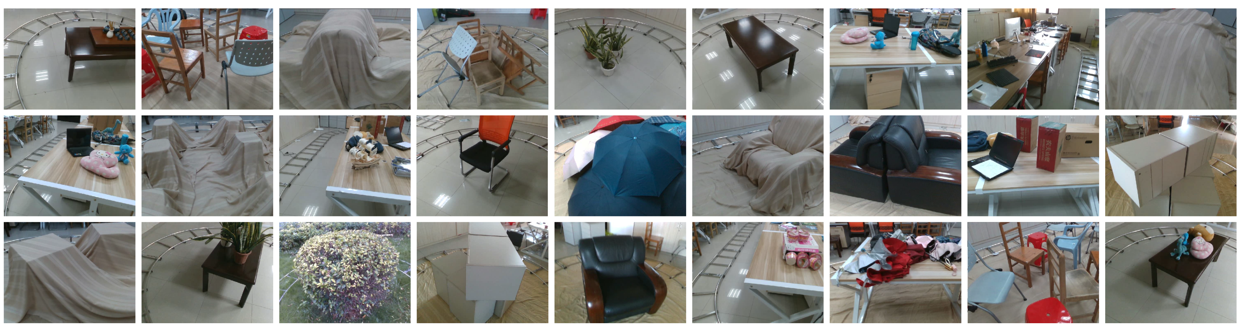
• Superior performance compared to advanced existing solutions, validated through extensive experiments on our open-source data sets captured using an Intel Realsense D435i. These data sets encompass RGB images (30 Hz), depth images (25 Hz), and IMU measurements (450 Hz) with fitted ground truth, covering multiple scenarios.
• A comprehensive evaluation of the VID-SLAM system using these diverse data sets, demonstrating its improved performance and reliability.

2. Methodology

The pipeline of VID-SLAM is illustrated in Figure 1. The system starts by receiving an RGB-D image paired with a corresponding sequence of IMU measurements, where the number of IMU measurements corresponds to the duration between consecutive RGB-D frames. These two types of data are processed separately. The IMU measurements undergo pre-integration to estimate the initial state, including position, velocity, and rotation changes, which are important for the initial alignment in the fusion process.

The features extracted from the RGB camera are tracked by the Kanade–Lucas–Tomasi (KLT) [18] sparse optical flow algorithm. IMU pre-integration [19] is performed over a certain number of IMU measurements. Then, the ICP algorithm is employed to estimate the rotation $\mathbf{R}\in \mathbb{S}{\mathbb{O}}_3$ and the translation $\mathbf{t}\in {\mathbb{R}}^3$ between consecutive depth maps.

In the following optimization procedure, the pose graph can be initialized using the pre-processed sensor states.

The optimization module tightly fuses geometric, IMU, and visual constraints to conduct non-linear optimization to search for the best solution. Last but not least, when a loop-closure is detected, the drift can be corrected by performing pose-graph optimization to ensure accurate localization in long-term running.

To be more specific, our approach encompasses four key components: (1) a Measurement Pre-processing Module, which processes raw inputs, converting them into structured data for subsequent processing; (2) the Robust Initialization Procedure, which aligns various measurements and establishes initial values essential for system calibration; (3) a Joint Estimation Module, a core component which integrates three types of constraints—namely visual, inertial, and geometric constraints—to accurately estimate the system’s state; and (4) a Loop Closure Module, which employs pose-graph optimization to correct cumulative errors and ensure the long-term stability of the system.

2.1. Measurement Pre-Processing

The measurement pre-processing used in this research is performed in real-time, and is similar to the pre-processing described in [8]. The RGB images and inertial measurements must be pre-processed before they can be converted into sensor states for subsequent modules. Specifically, we track visual features between consecutive colour frames and detect new features to improve the robustness of the system. The inertial measurements during the time interval between two consecutive frames will be pre-integrated using a real-time method to obtain a rough estimate of motion.

2.1.1. Visual Pre-Processing

We extract Shi–Tomasi features [20] from each RGB image and track these feature points using the KLT sparse optical flow algorithm [18]. As the tracking process contains noisy matches, outlier rejection is implemented using the RANSAC algorithm [21]. To ensure the accuracy and robustness of localization, new features are detected to maintain a minimum required number of tracked features.

Having visual features extracted and tracked, we need to decide whether the current frame is a new keyframe or not. For the insertion of keyframes, one of the following conditions must be satisfied:

• The average parallax from the previous keyframe is set to be higher than a threshold of 0.5 pixels, determined based on empirical testing to balance keyframe frequency and tracking stability.
• The system maintains tracking of at least 100 features in the current frame, a threshold chosen for optimal performance in varied environments as observed in preliminary tests.

2.1.2. Inertial Pre-Processing

In this step, we adopt the method from [8] for pre-integrating IMU measurements to propagate the states of position, velocity, and rotation. This process involves considering the time interval $[t_k,t_{k+1}]$ for IMU measurements and the corresponding image frames at instants $i_k$ and $i_{k+1}$. To accurately describe this state propagation, we refer to the following equation, which integrates various factors such as IMU measurements, biases, and gravitational effects over this interval.

$$\begin{array}{cc}\hfill & \begin{array}{cc}\hfill {\mathbf{p}}_{i_{k+1}}^w={\mathbf{p}}_{i_k}^w& +{\mathbf{v}}_{i_k}^w\Delta t_k\hfill \\ \hfill & +{\int \int }_{t\in \left[t_k,t_{k+1}\right]}\left({\mathbf{R}}_t^w\left({\widehat{\mathbf{a}}}_t-{\mathbf{b}}_{a_t}-{\mathbf{n}}_a\right)-{\mathbf{g}}^w\right)d{t}^2\hfill \end{array}\hfill \\ \hfill & {\mathbf{v}}_{i_{k+1}}^w={\mathbf{v}}_{i_k}^w+{\int }_{t\in \left[t_k,t_{k+1}\right]}\left({\mathbf{R}}_t^w\left({\widehat{\mathbf{a}}}_t-{\mathbf{b}}_{a_t}-{\mathbf{n}}_a\right)-{\mathbf{g}}^w\right)dt\hfill \\ \hfill & {\mathbf{q}}_{i_{k+1}}^w={\mathbf{q}}_{i_k}^w\otimes {\int }_{t\in \left[t_k,t_{k+1}\right]}\frac{1}{2}\Omega \left({\widehat{\omega }}_t-{\mathbf{b}}_{w_t}-{\mathbf{n}}_w\right){\mathbf{q}}_t^{i_k}dt,\hfill \end{array}$$

(1)

where ${\mathbf{R}}_t^w$ represents the rotation matrix transitioning from the IMU body coordinate frame to the world coordinate frame at any given time t. Specifically, $\mathbf{p}$, $\mathbf{v}$, and $\mathbf{q}$ denote position, velocity, and rotation, respectively. $\Delta t_k$ is the duration within the time interval $[t_k,t_{k+1}]$. $\omega$ and $\mathbf{a}$ are the gyroscope and accelerometer measurements from the IMU, respectively, while $\widehat{\omega }$ and $\widehat{\mathbf{a}}$ are their corrections which incorporate the force for countering gravity, bias, and additive noise. ${\mathbf{b}}_a$ and ${\mathbf{b}}_w$ are the acceleration and gyroscope biases, respectively. ${\mathbf{n}}_a\sim \mathcal{N}\left(\mathbf{0},{\sigma }_a^2\right)$ and ${\mathbf{n}}_w\sim \mathcal{N}\left(\mathbf{0},{\sigma }_w^2\right)$ are additive noises, assumed to be Gaussian distributions. ${\mathbf{g}}^w$ is the gravity vector. ${(·)}^w$ denotes the world frame. Moreover, the formulation incorporates $\Omega \left(\omega \right)$, a skew-symmetric matrix, which is defined as follows:

$$\Omega \left(\omega \right)=\left[\begin{array}{cc}-\lfloor \omega \rfloor \times & \omega \\ -{\omega }^T& 0\end{array}\right],{\lfloor \omega \rfloor }_{\times }=\left[\begin{array}{ccc}0& -{\omega }_z& {\omega }_y\\ {\omega }_z& 0& -{\omega }_x\\ -{\omega }_y& {\omega }_x& 0\end{array}\right].$$

(2)

2.2. Initialization

In the initialization phase of our Visual-Inertial-Depth Odometer (VIDO) system, accurate estimation of the initial state is important for precise state estimation. This phase involves combining the inertial data from the IMU with the visual data from the RGB-D camera to compute the initial gravity vector (${\mathbf{g}}^w$), the gyroscope bias (${\mathbf{b}}_g$), and the velocity of the system (${\mathbf{v}}^w$). First, we pre-integrate the IMU measurements between consecutive image frames to calculate the relative motion including rotation ($\Delta {\mathbf{q}}_{i_{k+1}}^{i_k}$) and translation ($\Delta {\mathbf{p}}_{i_{k+1}}^{i_k}$), a process that uses the gyroscope and accelerometer data over the time interval $[t_k,t_{k+1}]$. Meanwhile, a sliding-window-based structure-from-motion (SfM) technique is used to process a series of RGB-D images to estimate the initial camera pose and the geometry of the scene. The key step is to align the SfM results with the IMU pre-integrated data, which adjusts the scale of the trajectories obtained from the visual data and corrects them using the scale-aware properties of the IMU data. This alignment is accomplished by minimising the difference between the IMU pre-integrated results and the pose obtained by SfM, ensuring that our VIDO system has a stable and reliable initial state estimate.

2.3. Joint Estimation

For each new frame, we apply local non-linear optimization to refine the trajectory estimation. To improve the accuracy of localization with multiple sensory information, we proposed a sliding window-based Visual-Inertial-Depth Odometry (VIDO) that formulates a unique tightly coupled fusion of RGB-D and inertial estimates. The state vector of the sliding window is defined as

$$\begin{array}{cc}\hfill \mathcal{S}& =\left[{\mathbf{s}}_0,{\mathbf{s}}_1,\cdots {\mathbf{s}}_i,{\mathbf{T}}_c^b,{\lambda }_0,{\lambda }_1,\cdots {\lambda }_j\right]\hfill \\ \hfill {\mathbf{s}}_k& =\left[{\mathbf{p}}^w,{\mathbf{v}}^w,{\mathbf{q}}^w,{\mathbf{b}}_a,{\mathbf{b}}_g\right],k\in [0,i]\hfill \\ \hfill {\mathbf{T}}_c^b& =\left[{\mathbf{p}}_c^b,{\mathbf{q}}_c^b\right],\hfill \end{array}$$

(3)

where ${\mathbf{s}}_k$ is the IMU state of the $k\mathrm{th}$ keyframe. The first three items of ${\mathbf{s}}_k$ are the position, velocity, and rotation of the IMU, while the last two items of ${\mathbf{s}}_k$ are the acceleration bias and gyroscope bias in the IMU frame. i and j, respectively, denote the total numbers of keyframes and features. ${\mathbf{T}}_c^b\in \mathbb{S}{\mathbb{E}}_3$ denotes the transformation matrix from camera coordinates to IMU body coordinates. $\lambda$ refers to the inverse depth of features stored in the sliding window.

Our residual function consists of four terms: the sum of prior, the ICP errors, the IMU residual, and visual re-projection errors. We minimize the residuals to obtain the optimal estimation:

$$\begin{array}{cc}\hfill \underset{\mathcal{X}}{min}\left\{{∥{\mathbf{r}}_p-{\mathbf{H}}_p\mathcal{X}∥}^2+\sum _{(i,j)\in \mathcal{D}}{∥{\mathbf{r}}_{\mathcal{D}}\left({\widehat{\mathbf{z}}}_i^j,\mathcal{X}\right)∥}^2+\right.& \\ \hfill \sum _{k\in \mathcal{M}}{∥{\mathbf{r}}_{\mathcal{M}}\left({\widehat{\mathbf{z}}}_{m_{k+1}}^{m_k},\mathcal{X}\right)∥}_{{\mathbf{P}}_{m_{k+1}}^{m_k}}^2+\\ \hfill \left.\sum _{(k,j)\in \mathcal{V}}\rho \left({∥{\mathbf{r}}_{\mathcal{V}}\left({\widehat{\mathbf{z}}}_k^j,\mathcal{X}\right)∥}_{{\mathbf{P}}_k^j}^2\right)\right\},\end{array}$$

(4)

where

$$\rho \left(s\right)=log(1+s)$$

and ${\mathbf{r}}_p$ and ${\mathbf{H}}_p$ are the prior information from marginalization. $\mathcal{D}$ is the set of matched points between consecutive depth images, $\mathcal{M}$ is the set of all IMU measurements, and $\mathcal{V}$ is the set of features observed at least twice in the current sliding window. ${\mathbf{r}}_{\mathcal{D}}({\widehat{\mathbf{z}}}_i^j,\mathcal{X})$, ${\mathbf{r}}_{\mathcal{M}}({\widehat{\mathbf{z}}}_{m_{k+1}}^{m_k},\mathcal{X})$ and ${\mathbf{r}}_{\mathcal{V}}({\widehat{\mathbf{z}}}_i^{v_j},\mathcal{X})$ are the residuals of individual constraints. More details about these two residuals are provided in the subsequent sections. ${\mathbf{P}}_{m_{k+1}}^{m_k}$ and ${\mathbf{P}}_k^j$ are the corresponding covariance metrics. Ceres Solver [22] was used to solve this optimization task.

2.3.1. Geometric Constraint

Given two consecutive depth images, we estimate the relative transformation matrix between these images using the ICP algorithm. To improve the registration performance, we use a point-to-plane formulation [23], defined as

$${\mathbf{r}}_{\mathcal{D}}({\widehat{\mathbf{z}}}_i^j,\mathcal{X})=(\mathbf{T}·{\mathbf{P}}_j-{\mathbf{P}}_i)·{\mathbf{n}}_i,$$

(5)

where $\mathbf{T}\in \mathbb{S}{\mathbb{E}}_3$ is the transformation matrix, defined as

$$\mathbf{T}=\left[\begin{array}{cc}\mathbf{R}& \mathbf{t}\\ 0& 1\end{array}\right].$$

(6)

Here, ${\mathbf{P}}_i$ and ${\mathbf{P}}_j$ are matched 3D points from the respective depth images. $\mathbf{n}$ is the corresponding normal of the previous frame (${\mathbf{P}}_i$). The matrix $\mathbf{R}\in \mathbb{S}{\mathbb{O}}_3$ and vector $\mathbf{t}\in {\mathbb{R}}^3$ represent the rotation and translation from the coordinate system of the previous depth image (${\mathbf{P}}_i$) to the current depth image (${\mathbf{P}}_j$).

2.3.2. IMU Constraint

Given IMU measurements $m_k$ and $m_{k+1}$ within two consecutive frames, the residual of IMU pre-integration is defined as

$$\begin{array}{cc}\hfill & {\mathbf{r}}_{\mathcal{M}}({\widehat{\mathbf{z}}}_{m_{k+1}}^{m_k},\mathcal{X})=\left[\begin{array}{c}\delta {\alpha }_{m_{k+1}}^{m_k}\\ \delta {\beta }_{m_{k+1}}^{m_k}\\ \delta {\theta }_{m_{k+1}}^{m_k}\\ \delta {\mathbf{b}}_a\\ \delta {\mathbf{b}}_g\end{array}\right]=\hfill \\ \hfill & \left[\begin{array}{c}{\mathbf{R}}_w^{m_k}\left({\mathbf{p}}_{m_{k+1}}^w-{\mathbf{p}}_{m_k}^w+\frac{1}{2}{\mathbf{g}}^w\Delta t_k^2-{\mathbf{v}}_{m_k}^w\Delta t_k\right)-{\widehat{\alpha }}_{m_{k+1}}^{m_k}\\ {\mathbf{R}}_w^{m_k}\left({\mathbf{v}}_{m_{k+1}}^w+{\mathbf{g}}^w\Delta t_k-{\mathbf{v}}_{m_k}^w\right)-{\widehat{\beta }}_{m_{k+1}}^{m_k}\\ 2{\left[{\mathbf{q}}_{m_k}^{w^{-1}}\otimes {\mathbf{q}}_{m_{k+1}}^w\otimes {\left({\widehat{\gamma }}_{m_{k+1}}^{m_k}\right)}^{-1}\right]}_{\mathrm{m}}\\ {\mathbf{b}}_{a{m}_{k+1}}-{\mathbf{b}}_{a{m}_k}\\ {\mathbf{b}}_{w{m}_{k+1}}-{\mathbf{b}}_{w{m}_k}\end{array}\right],\hfill \end{array}$$

(7)

where ${\mathbf{R}}_w^{m_k}\in {\mathbb{SO}}_3$ is the rotation matrix from the world coordinate system to the IMU body coordinate system. $\Delta t$ is the time interval between two consecutive frames. ${\widehat{\alpha }}_{m_{k+1}}^{m_k}$, ${\widehat{\beta }}_{m_{k+1}}^{m_k}$, and ${\widehat{\gamma }}_{m_{k+1}}^{m_k}$ are the IMU pre-integration terms, which represent the integral prediction of the acceleration and angular velocity measured by the IMU from one frame to the next. These pre-integration terms are used to predict the changes in the IMU state (including position, velocity, and attitude) during this time period.

2.3.3. Visual Constraint

Similar to VINS, the re-projection error is defined on a unit sphere. Given a unit vector ${\mathcal{P}}_k^j$ that is back-projected from the pixel coordinates of the $k\mathrm{th}$ feature ${\mathbf{p}}_k$, and the corresponding 3D point that is predicted by transforming its first observation in the $i\mathrm{th}$ frame to the $j\mathrm{th}$ frame, we can define the visual residual r on the tangent plane of ${\mathcal{P}}_k^j$.

Bundle Adjustment (BA) is known to be a gold standard method which can produce jointly optimal 3D structures by refining a visual re-construction [24]. The re-projection errors of BA are defined on a generalized image plane for the most part. However, its traditional formulation may be less suitable for fisheye cameras, which require specialized calibration. Based on the main ideas of BA, we define the re-projection errors as our visual residual on a unit sphere, given as follows.

According to the pinhole camera model [25], the projection function $\pi :{\mathbb{R}}^3\to {\mathbb{R}}^2$ projects 3D points onto the 2D plane as follows:

$$\pi \left(\left[\begin{array}{c}X\hfill \\ Y\hfill \\ Z\hfill \end{array}\right]\right)=\left[\begin{array}{c}{f}_x\frac{X}{Z}+c_x\hfill \\ f_y\frac{Y}{Z}+c_y\hfill \end{array}\right],$$

(8)

where $(f_x,f_y)$ and $(c_x,c_y)$ are the camera’s intrinsic parameters, which are estimated through initial camera calibration and are assumed to be fixed throughout the keyframe sequence.

Given the $k\mathrm{th}$ feature ${\mathbf{p}}_k$ observed at least twice since its first appearance in the $i\mathrm{th}$ image, the corresponding 3D point in the unit sphere can be obtained as follows if this feature appears in the $j\mathrm{th}$ image:

$${\mathcal{P}}_k^j={\pi }_c^{-1}\left(\left[\begin{array}{c}{u}_k^j\\ v_k^j\end{array}\right]\right),$$

(9)

where $u_k^j$ and $v_k^j$ are pixel coordinates of feature ${\mathbf{p}}_k$ observed in the $j\mathrm{th}$ image. ${\pi }_c^{-1}$ turns pixel coordinates into a unit vector.

With the pixel coordinates of feature ${\mathbf{p}}_k$ observed in the $i\mathrm{th}$ image, we can obtain the corresponding 3D point in the world frame as follows:

$${\left({\mathcal{P}}_k^i\right)}^w={\mathbf{T}}_{w\leftarrow b_i}{\mathbf{T}}_{b\leftarrow c}\frac{1}{{\lambda }_k}{\pi }_c^{-1}\left(\left[\begin{array}{c}{u}_k^i\\ v_k^i\end{array}\right]\right)$$

(10)

$${\left({\mathcal{P}}_k^i\right)}^w={\mathbf{R}}_{b_i}^w\left({\mathbf{R}}_c^b\frac{1}{{\lambda }_k}{\pi }_c^{-1}\left(\left[\begin{array}{c}{u}_k^i\\ v_k^i\end{array}\right]\right)+{\mathbf{t}}_c^b\right)+{\mathbf{t}}_{b_i}^w,$$

(11)

where ${\mathbf{T}}_{w\leftarrow b_i}\in \mathbb{S}{\mathbb{E}}_3$ is the transformation matrix from the $i\mathrm{th}$ body frame to the world frame. ${\mathbf{T}}_{w\leftarrow b_i}$ consists of the rotation matrix ${\mathbf{R}}_{b_i}^w\in \mathbb{S}{\mathbb{O}}_3$ and translation matrix ${\mathbf{t}}_{b_i}^w\in {\mathbb{R}}^3$. ${\lambda }_k$, as used in (3), is the inverse depth of feature ${\mathbf{p}}_k$.

Similarly, we can predict the coordinates of the same 3D point in the $j\mathrm{th}$ body frame as follows:

$${\left({\mathcal{P}}_k^i\right)}^w={\mathbf{T}}_{w\leftarrow b_j}{\mathbf{T}}_{b\leftarrow c}\widehat{{\mathcal{P}}_k^j}$$

(12)

$${\left({\mathcal{P}}_k^i\right)}^w={\mathbf{R}}_{b_j}^w\left({\mathbf{R}}_c^b\widehat{{\mathcal{P}}_k^j}+{\mathbf{t}}_c^b\right)+{\mathbf{t}}_{b_j}^w.$$

(13)

We can summarize the expression of the prediction by referring to Equations (11)–(13):

$$\begin{array}{c}\hfill \widehat{{\mathcal{P}}_k^j}={\mathbf{R}}_b^c\left({\mathbf{R}}_w^{b_j}\right({\mathbf{R}}_{b_i}^w({\mathbf{R}}_c^b\frac{1}{{\lambda }_k}{\pi }_c^{-1}\left(\left[\begin{array}{c}{u}_k^i\\ v_k^i\end{array}\right]\right)+{\mathbf{t}}_c^b)\\ \hfill +{\mathbf{t}}_{b_i}^w-{\mathbf{t}}_{b_j}^w)-{\mathbf{t}}_c^b).\end{array}$$

(14)

In summary, we define our reprojection error as follows:

$${\mathbf{r}}_{\mathcal{V}}\left({\widehat{\mathbf{z}}}_k^j,\mathcal{X}\right)=\left[\begin{array}{c}{\overrightarrow{b}}_1\\ {\overrightarrow{b}}_2\end{array}\right]\left(\frac{\widehat{{\mathcal{P}}_k^j}}{∥\widehat{{\mathcal{P}}_k^j}∥}-{\mathcal{P}}_k^j\right),$$

(15)

where ${\overrightarrow{b}}_1$ and ${\overrightarrow{b}}_2$ are two orthogonal bases that can be found easily on the tangent plane of ${\mathcal{P}}_k^j$.

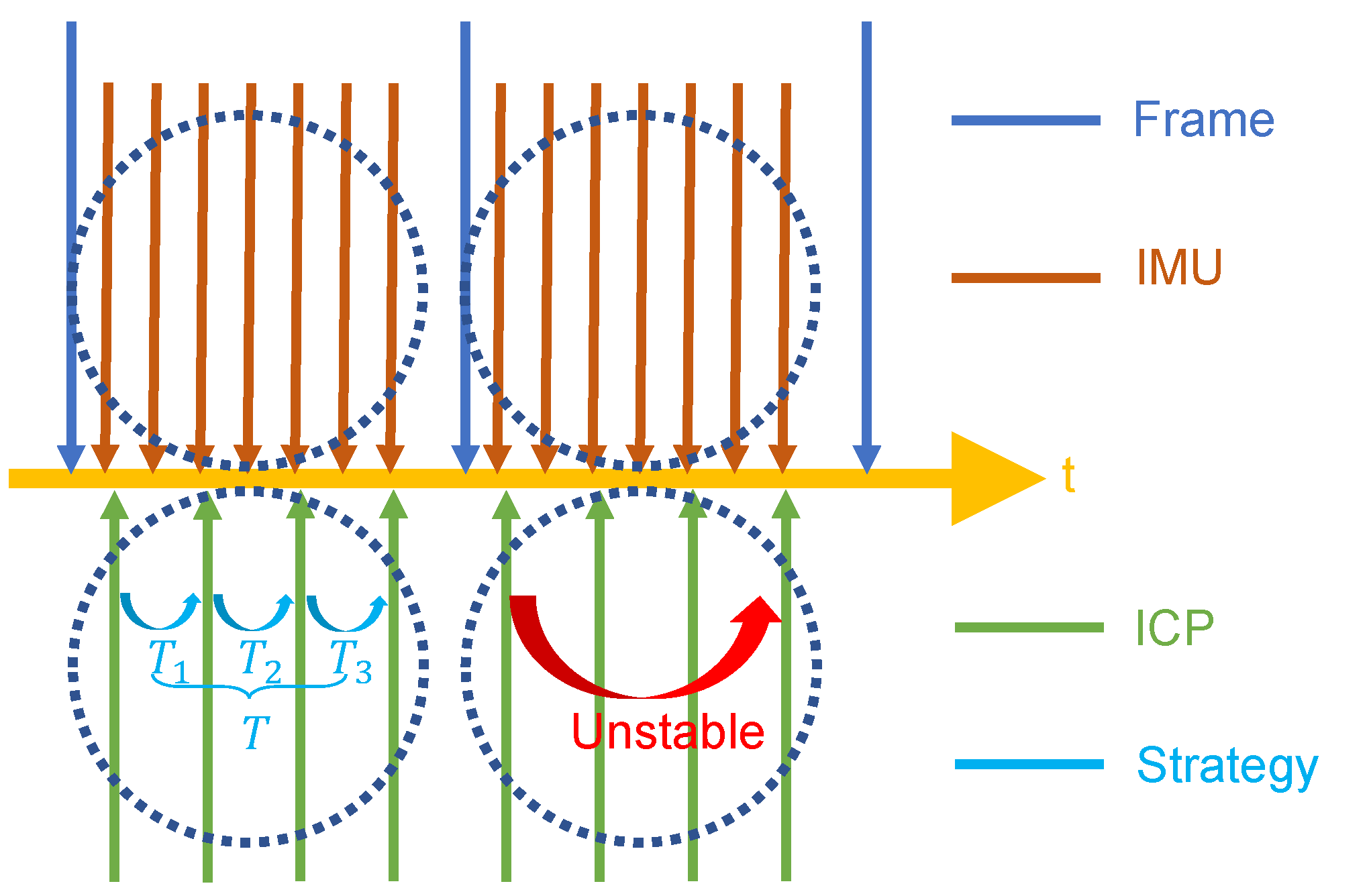
As shown in Figure 2, IMU pre-integration is performed over all measurements between every several RGB frames. ICP is applied to register every neighbouring frame.

To ensure real-time performance, we limit the number of iterations, as the system is designed for real-time deployment. As detailed in Section 3, this limitation allows us to perform fast estimation between two consecutive depth images. However, estimating motion between distant depth images with different 3D structures may affect the accuracy and computational cost.

2.4. Loop-Closure Detection

As accumulated drift is inevitable in the long-term running of SLAM systems, an approach based on Bag-of-Words (BoW) [26] is integrated to detect loop-closures. This approach queries the visual database with visual words (BRIEF descriptors [27] in our system) and returns loop candidates with the consistency verification.

If the current frame is selected as a keyframe, we extract BRIEF descriptors to validate loop closure. Pose-graph optimization is then performed to correct the accumulated drift after a validated loop closure.

It is worth noting that the loop-closure detection module is optional if the platform has limited computational resources. Thanks to the tightly coupled fusion strategy, our approach can achieve satisfactory localization performance in various environments even without loop-closure detection.

3. Experiments

3.1. Experimental Setup

3.1.1. Data Set

Synchronised sequences of RGB images, depth maps, and IMU measures are required to evaluate our system. As data of the required multi-sensors are not available in widely used public data sets such as the EuRoC MAV data set [28] and TUM data set [29], we collected an RGBD-inertial data set in various scenes using the Intel RealSense D435i device. The data set (https://jmueducn-my.sharepoint.com/:f:/g/personal/guikunchen_jmu_edu_cn/EmxU_0ZQMXVOvuKIdhxyOFgBJsM49OAH89j-JkOv-TH7RA (accessed on 16 June 2020)) and our source code (https://github.com/shawn87377/VID-SLAM (accessed on 16 June 2020)) have been released to the public.

In order to properly evaluate the performance of VID-SLAM, as shown in Figure 3, we built a playground-shaped rail and a circle-shaped rail as ground truth trajectories. During the process of creating the data sets, the device was fixed on the scaffold and recorded with a constant velocity.

The recorded data sets contained deformable and rigid body objects in various scenes, from flat to complex surfaces and from textured to textureless. Visually unsuitable conditions, such as textureless areas and fast-motion trajectories, make this data set a challenging benchmark for SLAM.

3.1.2. Platforms and Baselines

Our experiments were conducted on a computing platform equipped with an Intel Xeon E3-1225 CPU and an NVIDIA 1070 GPU. In order to implement state-of-the-art SLAM methods such as VINS-Mono (Qin2018vins), ElasticFusion (EF) (whelan2016elasticfusion), and ORB-SLAM2 (ORB2) (mur2017orb), we recommend that the system configuration include at least a quad-core processor and 4 GB of RAM in order to efficiently handle the computational demands.

Our experimental setup was carefully designed for rigorous testing, as shown in Figure 4. Figure 4a shows the Intel RealSense D435i camera used in the indoor experiment. The device was equipped with an integrated depth camera and a high-resolution RGB camera (640 × 480 pixels), as well as a built-in IMU capable of 6DoF motion detection, which is necessary for accurate pose estimation and motion tracking. Figure 4b depicts a customised track, which was used to ensure controlled and repeatable camera motion. The design of the track helps to achieve consistent movement speeds and trajectories, which is important for benchmarking the performance of the SLAM algorithm.

3.2. Results and Discussions

3.2.1. Overall Evaluation

On the basis of the degree of the complexity of the textures and surfaces, the data set consisted of four sub-data sets (see

Table 1. RMSE of experimental method without loop closure.

Classification	Sequence	RMSE (m)
		VINS-Mono	ORB2	EF	Ours
	c-boxes	0.583	0.02	0.01	0.012
Flat Surface and	p-boxes	0.038	0.046	0.031	0.022
Textured	p-desk1	0.057	0.035	0.049	0.023
	c-boxes*	0.319	0.016	0.017	0.018
Flat Surface and	p-boxes*	0.984	0.037	0.043	0.022
Textureless	p-desk1*	0.857	0.048	0.011	0.018
	p-umbrella	0.113	0.047	0.126	0.031
Complex Surface	p-chairs1	0.596	0.081	0.101	0.025
and Textured	p-chairs2	0.092	0.045	0.055	0.024
	p-umbrella*	0.061	x	0.268	0.027
Complex Surface	p-chairs1*	0.18	x	0.131	0.039
and Textureless	p-chairs2*	0.089	0.058	0.031	0.026

). With respect to the surface appearance, scenes with boxes and desks were grouped as a flat-surface data set, while scenes with umbrellas and chairs were considered as a complex-surface data set. In the table, ‘c’ denotes a circle-shaped rail data set, ‘p’ denotes a playground-shaped rail data set, ‘*’ denotes a data set using striped fabric for covering (to construct a textureless surface), and ‘x’ denotes tracking failure.

As the lab had no GPS-RTK to measured ground truth paths, we built the data sets following fixed trajectories and, by this means, we could visually inspect whether the trajectory was fitted but could also easily generate precise ground truth trajectories. Note that the ground truth is two-dimensional, while the experimental results are three-dimensional. For fair comparison, we evaluated the projection trajectories of each system. Having each experimental result aligned with its corresponding ground-truth trajectory, we used the root-mean-square error to measure the performance of different methods. A smaller RMSE value means that the trajectory aligned to the ground truth better. In order to highlight the comparisons, we compared the absolute translation in the odometry-only experiment.

From Table 1, we can observe that VID-SLAM achieved a better and more stable performance in most cases. It is worth noting that ORB-SLAM2 had estimation failure in the p-chairs1* and p-umbrella* data sets. This phenomenon indicates that texture has a greater impact on ORB-SLAM2 under complex circumstance. As relatively accurate feature points can be extracted in textured scenes, Oriented FAST- and Rotated BRIEF-based algorithms always performed well in terms of feature point matching. Conversely, tracking loss may occur in textureless areas, where the accuracy and number of feature points are insufficient.

In particular, the RMSE results show that it is a challenging task for VINS-Mono to estimate its state when it is under complex and textureless environments (even without loop closure). Comparing the results of textured scenes and textureless scenes, we can empirically observe that the RGBD-based odometry is less accurate in complex scenes, even they have rich textures. It is worth noting that ElasticFusion was more stable than ORB-SLAM2, due to the high weight of its ICP results. However, it still drifted a lot when we disabled its loop detection.

3.2.2. Typical Scenes Analysis

In Figure 5, the trajectories of different SLAM methods are compared, where the red dashed line represents the ground truth, the blue solid line represents the trajectory estimated by the VINS-Mono algorithm, the purple solid line is for the ElasticFusion algorithm, the green solid line denotes the ORB-SLAM2 algorithm and, importantly, VID-SLAM is represented by the orange solid line. As shown in Figure 5, our VID-SLAM approach outperformed the baselines in the sequence p-sofa*, especially in cases without loop closure. The intuitive comparison of trajectories in Figure 5a highlights that VID-SLAM’s trajectory closely aligned with the ground truth. Figure 5c,d depict the absolute scale drift variation over distance (time). While VINS-Mono exhibited considerable drift due to initial scale inaccuracy, our VID-SLAM achieved an RMSE of 0.017 without loop closure detection and 0.014 with loop closure detection.

The main purpose of this part was to evaluate the generality of the system. The common features of typical sequences are localization-friendly, such as textured areas, dissimilar features (descriptors), moderate motion velocity, clear illumination, and so on. These features meet the assumptions of SLAM systems and enable them to operate regularly. The front-end of the SLAM system could be comprehensively evaluated in such sequences as those mentioned above.

Except for VINS-Mono, the p-sofa* sequence could be estimated well by all of the evaluated systems. For SLAM systems, the p-sofa* sequence is a typical and simple scene, as environments with distinguishable features and clear illumination make feature tracking more achievable.

As the vision processing front-end is an important component of VINS-Mono, it will directly affect the estimation quality if specific scenarios cause SfM failure. Figure 5b shows flexible objects covered with striped fabric. These similar features can cause inaccurate initialization, leading to a loss of metric scale. This is why the trajectory of VINS-Mono had the right trend, but lost its scale.

The results of ElasticFusion and ORB-SLAM2 exhibited obvious drift when we disabled loop detection. The odometry of these RGB-D methods utilizes geometric and photometric information to estimate the most suitable motion parameters (i.e., rotation and translation) between two consecutive frames by minimizing the joint cost function.

It can be observed that the trajectories of each system are close to the expected shape from the tendency. However, only VID-SLAM could maintain accurate global estimation during long-term localization without the loop closure module.

To fully evaluate the performance of our system in various conditions, we also recorded challenging scenes. As Figure 6b shows, this scene had many different chairs that were arranged in a disorderly manner, and its textureless areas make camera tracking more difficult. This scene has very similar features and non-uniform depth information. Our experimental results are shown in Figure 6. Detailed discussions are given as follows.

We observed that VINS-Mono had a problem of scale inconsistency in Figure 6a. The Inertial Measurement Unit (IMU) is easily affected by noise, especially when using low-cost IMUs. Therefore, the results of the scale estimation of VINS-Mono were far from stable and precise. Furthermore, the loop closure of VINS-Mono depends on both vision and pose, and it also failed due to its previous misestimation.

Compared to VINS-Mono, ElasticFusion and ORB-SLAM2 had impressive performance in this scene when using loop closure. However, they both drifted significantly when we disabled the loop detection. Note that our approach combines RGB-D sensors with IMUs for visual SLAM, which estimates more reliable camera poses by optimizing residuals that consist of multiple constraints.

Our approach achieved promising results in both typical and challenging scenes. The experimental results indicated that our multi-sensor fusion strategy could make a trade-off of metric scale and accuracy, dramatically improving its state estimation performance. Besides this, VID-SLAM still worked well in challenging scenes and achieved accurate localization even without loop closure.

3.2.3. Challenging Scenes Analysis

This evaluation used a small-scale circular rail to circle the boxes. The box is considered a relatively simple structure with a flat and textureless surface. The additional use of striped fabric complicated the texture structure in the c-boxes* scene. From Figure 7 and Figure 8, it can be seen that the degree of trajectory drift of the Vins-Mono system improved (RMSE decreased from 0.583 to 0.319) when the scene switched from c-boxes to c-boxes*. This is because feature matching is easier and more accurate in the c-boxes* scene than in c-boxes. Inaccurate matching interferes with Visual-Inertial odometry. Therefore, in large scenes, the Vins-mono system will drift more significantly, and this error is difficult to eliminate even with loop closure. Compared with other systems, the RGBD-based approach and VID-SLAM achieved robust results, with RMSE close to 0.01 in both loop and non-loop experiments. This indicates that it is valuable to introduce depth information to constrain the estimation results of other sensors.

By comparing Figure 9a with Figure 10a, we can observe that, in the Figure 9b scene, which is richer in texture features, the RMSE obtained by the VIO-based Vins algorithm evaluation was significantly lower than that in the Figure 10b scene. This is mainly due to the fact that VIO-based algorithms are highly dependent on feature matching, and such algorithms have difficulty performing accurate bit-pose estimation in scenes with weak textures. In contrast, the overall RMSE estimation results of other computation methods that take depth information into account were not significantly affected by texture variations.

Figure 10 indicates that the added striped fabric hid the distinct colour attributes and changed the depth distribution of the original scene. This inevitably causes interference in the VIO-based algorithm if the extracted feature points of the scene become difficult to estimate and match. The RMSE of Vins-Mono increased significantly (from 0.074 to 0.354) when the loop closure was not used. As for ElasticFusion, which relies on the iterative closest point method and photometric error minimization, it was still affected in such scenarios. It is worth mentioning that bundle adjustment can optimize variables such as the camera poses and the observed structure relatively well, and the generated trajectory of ORBSLAM2 did not present any significant drift. VID-SLAM performed efficient Visual-Inertial-Depth odometry, and achieved a similar RMSE as ORBSLAM2 when there was no loop closure, but outperformed ORBSLAM2 with loop closure.

The playground-shaped rail is considered a long-distance test option in our experiment. As shown in Figure 11 and Figure 12, the chairs in both scenarios resulted in more depth noise, and they were not scenes with rich texture. RGBD-based SLAM systems will encounter more challenges under this circumstance. As can be seen from the experimental results, the trajectories of ElasticFusion and ORBSLAM2 drifted a short distance when the system did not detect loop closures. Furthermore, an obvious loss of scale appeared in the trajectory of Vins-mono. Note that a visually appealing trajectory was produced by VID-SLAM, as we effectively introduce IMU data to add constraints for the RGBD-based localization estimation.

3.2.4. Real-Time Performance Analysis

In fields such as robotics, SLAM systems require not only accurate localization but also focus on real-time performance. In this section, the runtime of each major part of our system is analysed in detail.

As shown in

Table 2. Main step times in p_umbrella sequence.

Steps	Median (ms)	Mean (ms)
Feature Tracker	4.86	7.87
Outlier Rejection	6.28	6.42
Keyframe Insertion	2.91	2.98
Iterative Closest Point	11.53	11.38
Joint Estimation	77.93	81.90
Pose-Graph Optimization	38.57	32.16

, our system consists of several different phases, each of which is characterised by a specific time consumption. The processing time of the feature tracker varies depending on the complexity of the scene and the speed of motion, with a median of 4.86 ms and a mean of 7.87 ms, reflecting its ability to maintain tracking accuracy in different environments. The Outlier rejection step had a median of 6.28 ms and a mean of 6.42 ms, and is a process that is important to exclude false feature matches in order to ensure the accuracy of subsequent calculations. Keyframe insertion had a shorter runtime, with median and mean values of 2.91 ms and 2.98 ms, respectively, which reflects the efficiency of our system in adding new keyframes. The ICP algorithm estimates the iterative direction, which had a median of 11.53 ms and a mean of 11.38 ms, which reflects the ICP algorithm’s ability to ensure bit-position estimation accuracy. Joint estimation, the central part of the SLAM system, is the step that took the longest, with a median of 77.93 ms and a mean of 81.90 ms. This process is performed by combining a variety of constraints to form the residual function, which is solved by the Ceres non-linear optimization solver, and its long runtime reflects the computationally demanding nature of the process required to sustain the the computational effort required for highly accurate state estimation. Pose-graph optimization is crucial in the global loop closure module, with a median of 38.57 ms and a mean of 32.16 ms, which is executed only after loop closure has been confirmed, giving a runtime that varies depending on the complexity of the scenario.

4. Conclusions and Future Work

4.1. Conclusions

In this paper, we proposed a reliable and robust approach called VID-SLAM that fuses multi-sensor information (RGB-D and IMU) to improve the camera pose estimation performance. We first designed RGB-depth-inertial data sets for comprehensive evaluation. Based on tightly coupled visual-inertial-depth odometry, we presented a cascaded cost function to fuse multiple sensor states and a stable system with loop detection and pose-graph optimization. The experimental results conducted on our data set indicated that the proposed VID-SLAM significantly outperforms the other methods, including VINS-Mono, ElasticFusion, and ORB-SLAM2.

Notably, while our approach presented improved accuracy and robustness in challenging environments, it still has some limitations. For example, the complexity of the cascaded cost function and the need for multiple sensors may increase the associated computational requirements, which may affect the efficiency of real-time applications. In addition, our current system is optimized for environments where reliable RGB-D and IMU data are available, and it may be limited in application scenarios with poor sensor accuracy.

4.2. Future Work

The localization performance of our system is robust and accurate, but there is still room to improve it, provided that more information about the environment can be perceived. Our sensor fusion method is generic, and the proposed multi-sensor formulation is a trade-off between accuracy and efficiency for our hardware settings. Therefore, we can upgrade the combination of sensors for more accurate localization. The robustness of our system could also be improved. Although our work mainly focuses on the accuracy of localization, a more advanced re-localization module may improve not only the robustness of the system but also the accuracy of localization. A further potential improvement is the integration of dense mapping with our system; that is, we can improve the map representation by exploiting the ability to construct detailed and dynamically updated 3D maps from RGB-D data. This process involves synchronising depth data from RGB-D sensors with attitude estimates from SLAM systems. By doing so, we can generate dense, textured 3D maps, enabling further applications.