Dynamic Partitioning of Graphs Based on Multivariate Blood Glucose Data—A Graph Neural Network Model for Diabetes Prediction

Abstract

Postprandial Hyperglycemia (PPHG) persistently threatens patients’ health. Therefore, accurate diabetes prediction is crucial for effective blood glucose management. Most current methods primarily focus on analyzing univariate blood glucose data using traditional neural networks, neglecting the importance of spatiotemporal modeling of multivariate data at the node and subgraph levels. This study aimed to evaluate the accuracy of using deep learning (DL) techniques to predict diabetes based on multivariable blood glucose data, aiming to improve resource allocation and decision-making in healthcare. We introduce a Nonlinear Aggregated Graph Neural Network (NLAGNN) that utilizes continuous multivariate historical blood glucose data from multiple patients to predict blood glucose levels over time, addressing the challenge of accurately extracting strong and weak correlation features. We preliminarily propose a Nonlinear Fourier Graph Neural Operator (NFGO) for nonlinear node representation, which effectively reduces meaningless noise. Additionally, a dynamic partitioning of graphs is introduced, which divides the a hypergraph into distinct subgraphs, enabling the further processing of strongly correlated features at the node and subgraph levels, ultimately obtaining the final prediction through layer aggregation. Extensive experiments on three datasets show that our proposed method achieves competitive results compared to existing advanced methods.

1. Introduction

The vast potential of artificial intelligence in healthcare presents promising prospects for diabetes diagnosis. The International Diabetes Federation (IDF) reported in the 10th edition of the “IDF Diabetes Atlas” that in 2021, 537 million people worldwide were living with diabetes, and this number is expected to reach 643 million by 2030 and 783 million by 2045 [1]. Diabetes mellitus (DM) is a chronic metabolic disorder characterized by a deficiency in insulin secretion (Type 1 Diabetes, T1D) or defects in insulin secretion and action (Type 2 Diabetes, T2D), which prevents patients from naturally regulating their blood glucose (BG) levels. Managing diabetes in daily life presents a fundamental challenge for patients, necessitating lifestyle changes and the development of self-care skills for effective blood glucose control. Without these measures, patients face an increased risk of long-term complications, including hypertension and cardiovascular issues. To maintain near-normal glucose levels, patients with Type 1 diabetes typically use an insulin pump or administer insulin via injections. Regular monitoring of blood glucose helps prevent acute complications of T1D, such as hypoglycemia and hyperglycemia. Hypoglycemia can increase the risk of both short-term and long-term mortality. Hyperglycemia can lead to cognitive decline, dysfunction, emotional disorders, and obstructive sleep apnea, as well as complications like liver disease, kidney disease, cardiovascular disease, and retinopathy [2,3,4]. Patients can perform self-monitoring of blood glucose (SMBG) using finger-stick glucometers for multiple daily measurements. However, blood glucose fluctuations caused by external factors cannot be detected accurately by this method. Technological advancements have spurred the development of the artificial pancreas (AP), a system that includes an automatic insulin control system, an insulin pump, and continuous glucose monitoring (CGM). In an artificial pancreas system, CGM continuously tracks a patient’s blood glucose levels and transmits the data to an automated insulin control system. This system calculates the necessary insulin dosage to regulate glucose balance using internal heuristic algorithms and prior knowledge. As a result, the artificial pancreas can automatically adjust insulin infusion doses while continuously monitoring glucose levels, thereby preventing hypoglycemia and hyperglycemia. This capability makes the AP a crucial solution for treating T1D. However, the AP is not a fully automated closed-loop system [5]. The delayed absorption effect of insulin in the body and other physiological factors make it difficult to precisely simulate blood glucose levels, leading to inaccurate insulin dosage [6]. Therefore, predicting future blood glucose values has become essential, which helps prevent T1D complications while improving the quality of life and health of patients [7].

A great number of studies have been dedicated to developing blood glucose prediction models, making data-driven methods the predominant approach. These techniques often rely on machine learning models, which have demonstrated excellent performance in predicting diabetes [8]. For example, S. Langarica et al. [9] estimated uncertainty in predictions using the Input and State Recurrent Kalman Network (ISRKN), which integrates input and state Kalman filters into the latent space of a deep neural network to address blood glucose prediction for Type 1 diabetes patients under meal uncertainty. K. Li et al. [10] proposed the Fast Adaptive and Confident Neural Network (FCNN) and applied model-agnostic meta-learning to rapidly adapt to new T1D subjects with limited training data. They successfully predicted blood glucose levels for 12 T1D patients within 30- and 60-min prediction windows. Bogdan-Petru Butunoi et al. [11] selected four models (ARIMA, RNN, LSTM, and GRU), determined the optimal order for the ARIMA model, and utilized the other three networks to capture time and data patterns for evaluating blood glucose prediction performance. To further improve model performance, researchers have discussed the optimal number of features for each patient. Martinsson et al. [12] applied Long Short-Term Memory (LSTM) networks to predict blood glucose levels for the next 30 to 60 min. Simon Y. Foo et al. [13] conducted a study using seven machine learning (ML) algorithms to analyze the Pima Indian Diabetes (PID) dataset from the UCI repository. The study showed that models based on Logistic Regression (LR) and Support Vector Machine (SVM) achieved an 88.6% accuracy in predicting diabetes. Usama Ahmed et al. [14] integrated the SVM and Artificial Neural Network (ANN) models and further combined them with a fuzzy model, employing fuzzy logic to classify positive and negative diabetes cases. Sihao Wang et al. [15] developed a LASSO (Least Absolute Shrinkage and Selection Operator) regression model that efficiently handles high-dimensional data and reduces the risk of overfitting, demonstrating strong predictive accuracy and interpretability. However, these methods overlook the continuity of attributes and the varying degrees of correlation among variables.

To address the aforementioned challenges, a novel deep learning network, Non-linear Aggregated Graph Neural Network (NLAGNN), is proposed in our study. The NLAGNN explicitly decomposes the input data into various subgraphs by applying generative component representations on a hypergraph, based on which analytical tasks are accomplished. In the NLAGNN, data are modeled as a hypergraph [16], with representations of different nodes nonlinearly transformed and values reassigned along the temporal dimension for multi-input sequences. On the foundation of prior work, hypergraphs are segmented into subgraphs of diverse scales, adeptly resolving the challenge of extracting information on variable interdependencies. To better capture the information in different subgraphs, a layer aggregation method is developed to consolidate both intra-variable and inter-variable information within sub-layers. Our main contributions are as follows:

• A novel deep learning network, NLAGNN, is introduced, which represents data as a hypergraph. This approach addresses the challenge of capturing temporal and spatial dynamics in blood glucose data, including patient-specific dependencies. In addition, a novel Non-linear Fourier Graph Neural Operator (NFGO) is introduced, which enhances variables strongly correlated with blood glucose and appropriately masks irrelevant features.
• Accordingly, a dynamic subgraph partitioning approach is devised, which further enhances the semantic information of nodes within regions of strongly correlated variables using different subgraphs in combination with multi-convolutional kernels for adaptive feature selection.
• In the realm of blood sugar forecasting, our model was rigorously assessed through extensive experiments on three authentic blood glucose datasets [17,18,19]. The experimental outcomes demonstrate that the NLAGNN outperforms other advanced methods, achieving competitive results.

2. Related Work

2.1. Methods of Blood Glucose Forecasting

Accurate blood glucose prediction is crucial for effective diabetes management, especially for patients in intensive care units (ICUs) where blood glucose is measured irregularly [20]. Continuous-time recurrent neural networks (CTRNNs) have shown promise in predicting irregularly measured blood glucose levels. These networks interpret irregular glucose observations through the continuous evolution of hidden states using ordinary differential equations (ODEs) or neural flow layers, ultimately predicting blood glucose using electronic medical records and data. Harleen Kaur et al. [21] developed and analyzed five supervised machine learning algorithms using R data manipulation tools: linear kernel support vector machine (SVM-linear), radial basis function (RBF) kernel support vector machine, k-nearest neighbor (k-NN), artificial neural network (ANN), and multifactor dimensionality reduction (MDR), to detect risk factor patterns in the Pima Indian diabetes dataset. Khadem et al. [22] proposed an interconnected lag fusion framework based on nested meta-learning, thus addressing the challenge of determining the optimal retrospective window length. This approach adapts to individual-specific predictive needs and optimizes the selection of the lag window, thereby improving the precision of personalized blood glucose predictions. De Bois et al. [23] introduced the GLYFE (GLYcemia Forecasting Evaluation) benchmark to address sensitivity issues associated with T1D data, difficulties in sharing data across studies, and variability in data processing procedures. This benchmark aims to evaluate various blood glucose prediction models and increase transparency by comparing their clinical applicability. Li et al. [24] conducted high-precision predictions of blood glucose levels in both simulated and real T1D patients at different time spans (30 and 60 min) using Convolutional Recurrent Neural Networks (CRNNs), with an accuracy measured by the Root Mean Square Error (RMSE). Jacopo Pavan et al. [25] selected two neural networks with similar prediction accuracies (p-LSTM and np-LSTM) and used the SHAP interpretability tool to analyze their outputs. The results revealed that only p-LSTM learned the physiological relationship between input data and glucose prediction. With accuracy confirmed, the study focused on evaluating the model’s stability and physiological validity through interpretability, aiming to integrate it into decision support systems (DSS) for corrective insulin bolus (CIB) recommendations. Saúl Langarica et al. [26] proposed an accurate personalized modeling technique based on meta-learning, requiring minimal data to adapt from its population version, with few training iterations and a low risk of overfitting. Results from the UVa/Padova Type 1 Diabetes Mellitus Metabolic Simulator (T1DMS) showed improved generalization in specific task metrics. However, previous methods have tended to overlook the potential value between multiple variables, and relatively little work has been done in this area.

2.2. Graph Neural Networks for Multivariate Time Series Forecasting

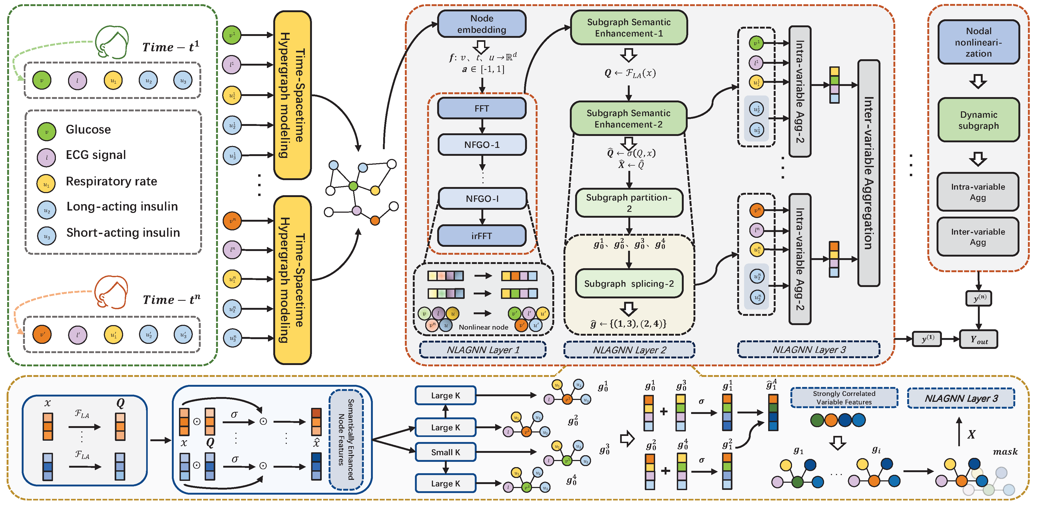
When dealing with multivariate time series (MTS) data, traditional methods focus primarily on the correlations between timestamps due to the fixed sequential structure of MTS data, which is usually implemented through temporal encoders such as Transformers, CNNs, and LSTMs. LSTMs [27], with three gating mechanisms, can capture long-term dependencies by maintaining states across different time steps, which makes them suitable for classification and prediction tasks in complex systems. Initially designed for image processing, CNNs are also used in finance, sensor analysis, and healthcare. They treat time series as one-dimensional spatial signals and capture local dependencies among multiple data through convolutional layers, effectively treating MTS data as two-dimensional images [28]. Transformers [29] learn long-distance temporal dynamics and interactions between variables through their self-attention mechanism, which is useful in tasks such as traffic flow prediction and energy consumption forecasting. Although traditional neural networks have made progress in capturing both short- and long-distance dependencies, they are constrained by the fixed size and structure of the data, and their ability to capture long-term dependencies remains limited. In more complex MTS data, the performance of traditional neural networks tends to decline.

In recent years, Graph Neural Networks (GNNs) have been successfully applied to various tasks based on graph structures [30], including node classification and link prediction of MTS data. Models like STGCN [31], DCRNN [32], and TAMP-S2GCNet [33] typically require predefined graph structures. However, the graph structure is often unknown. To address this limitation, some studies have learned the associations between sequences through self-attention mechanisms or node similarity to automatically represent the graph structure. Other methods use separate temporal and graph networks to deal with spatiotemporal correlations. For example, 1D-CNNs [34] leverage GNNs and CNNs to capture spatial and temporal dependencies, respectively. In 2021, Li et al. [35] employed LSTM networks as temporal feature extractors, integrating them with GNNs to construct graph structures. Renhe Jiang et al. [36] proposed a meta-graph learning mechanism based on spatiotemporal data to address the spatiotemporal heterogeneity and non-stationarity of traffic flow. A comprehensive evaluation on three traffic datasets, supported by qualitative assessments, demonstrated the model’s effectiveness in distinguishing different road connection patterns. While these methods strengthen the spatiotemporal correlation, they fail to fully unify the spatiotemporal aspects because dependencies are captured independently in two separate networks. Furthermore, these methods have not yet been used to analyze the strength of correlations among neighboring nodes in multiple variables from the perspectives of nodes and layers.

3. Methodology

Definition 1.

Problem formulation.

In multivariate blood glucose prediction, $x_{\mathrm{t},\mathrm{k}}\in {\mathbb{R}}^{N\times D}$ signifies the value of the nth variable in a k-variable set at time step t, originating from a sequence of N variables with a feature dimension D. A retrospective window, sized $X_{T,K}=\{x_{t-L,0},x_{t-L+1,1},\cdots ,x_{t,k}\}$, is defined, encompassing previous blood glucose observations. This window reflects the glucose trajectory for variable n at time node $\tau$, spanning from $t-L$ to $t-1$, where L represents the window extent, and t denotes the start of the prediction window. The goal of multivariate blood glucose prediction is to predict the forthcoming values of N variables across future T time steps. The comprehensive predictive function is articulated below, with ${\mathcal{F}}_{\mathcal{G}}$ denoting the operational mechanism of the graph network:

$${\widehat{Y}}_t={\mathcal{F}}_G(x_{t+1},x_{t+2},\dots ,x_{t+n})$$

(1)

Definition 2.

HyperGraph.

The intricacies of multivariate blood glucose sequence analysis are studied in-depth using graph theory. Variables are encapsulated as nodes within a graph, and inter-variable correlations are depicted through an adjacency matrix A, thus enhancing the efficacy of the analysis. An input retrospective window, denoted as $X_{T,K}\in {\mathbb{R}}^{N\times D}$, of the multivariate blood glucose observations is utilized. From this, a hypergraph $H_{\mathcal{G},T}=(X_T,E_T)$ with $N\times D$ nodes is meticulously constructed. Each element of $X_{T,K}$ is recognized as a node within the set $H_{\mathcal{G},T}$, where $X_T\in {\mathbb{R}}^{N\times D}$ denotes the node set across T time points, while $E_T\in {\mathbb{R}}^{ND\times ND}$ signifies the edge set in the same temporal scope. Owing to $E_T\in A_T$, the structure of the hypergraph is re-envisioned as ${\mathcal{G}}_T=(X_T,A_T)$. The initial adjacency matrix for T time points is represented by $A_T$, rendering ${\mathcal{G}}_T$ a fully connected graph. Here, the adjacency matrix describes the connections between nodes in a graph, with element values representing the weights of the edges between nodes.

3.1. Technical Roadmap

Currently, most methods focus on processing univariate data, using neural networks to model time-series data with seasonality and periodicity, while few studies have investigated feature learning for multivariate blood glucose data. We observed that previous research often modeled time and space separately before integrating them, which disrupts their original correlation, complicating reconciliation in subsequent analyses. To address these challenges, we outline our approach in the following steps:

1.

To emphasize the importance of spatiotemporal modeling, we represent the variable and time data as a hypergraph structure. In this structure, the central node (blood glucose) is connected to several other variable nodes via hyperedges, representing their relationships through multiple edges extending from the same node.

2.

Our proposed Nonlinear Fourier Graph Neural Operator (NFGO) represents the nodes in the hypergraph nonlinearly, aiming to capture the feature intensities of multiple variables while reducing meaningless noise.

3.

After applying semantic enhancement to the nodes in the hypergraph, we use fuse the convolution to adaptively reconstruct the adjacency matrix weights, dynamically partitioning the hypergraph into multiple subgraphs and extracting features at the subgraph level. Details of this section are found in the second layer of Figure 1.

4.

To effectively aggregate the features obtained from the previous steps, we use intra-variable and inter-variable aggregation methods to reconstruct the feature maps from different pieces of node information across the three branches, thereby predicting the final blood glucose values.

3.2. Nonlinear Node Representation of Hypergraph

In multivariate blood glucose datasets, there are certain variables that are weakly correlated with blood glucose, such as body posture. When these variable attributes are used as inputs, existing methods based on additive aggregation strategies may lead to the generation of meaningless features. For example, without considering the uneven distribution of variable attribute values across different consecutive timestamps, patients develop postprandial hyperglycemia, and directly calculating the average blood glucose of different patients may produce many features that are poorly correlated with actual blood glucose values, which will disrupt the probability distribution in blood glucose prediction, affect doctors’ judgment of results, and lead to incorrect treatment plans for patients. To solve this problem, the Graph Neural Operator (GNO) is proposed, which can locally activate nodes of strongly correlated variables nonlinearly. This process effectively represents the features of the corresponding strongly correlated variables, cleverly associates them locally with the features of blood glucose variables, and appropriately masks weakly correlated or uncorrelated features. Given a graph $G(X,A)$, an adjacency matrix $A\in {\mathbb{R}}^{n\times n}$, and a node feature $X\in {\mathbb{R}}^{n\times d}$, the form of GNO is as follows:

$$o_{GNO}=\mathrm{\Theta }(X,A_i,W_i,r_i)$$

(2)

In a single multi-attribute graph, the framework is segmented into several layers along the channel dimension, where r denotes the bias and W signifies the weight matrix. Each layer is initially scrutinized in isolation, endowing each node with a vectorial representation. Drawing inspiration from [30], it is proposed that the graph progressively captures representations of nodes associated with strongly correlated variables, such as insulin, during the learning process. Ideally, the features extracted from this graph should show a pronounced response at the insulin node positions, characterized by large vector magnitudes and aligned directions among insulin and blood glucose nodes. Conversely, other positions and irrelevant variables should exhibit minimal activation, essentially becoming null vectors.

In our methodology, the propagation mechanism of graph convolutional networks is integrated into a stratified graph architecture. A nonlinear function is introduced to serve as the non-linear node representation within the GNO. The formulation of the NFGO is delineated as follows:

$$o_{NFGO,*}=\bigcup _{k=0}^K\sigma ({\displaystyle \frac{e^{\alpha A_{i}X{W}_i}}{{\sum }_{i=1}^n{e}^{\alpha A_{i}X{W}_i}}}+r_i),\alpha >0$$

(3)

$$x^{\prime }=\{x_1{o}_{NFGO,1},x_2{o}_{NFGO,2},...,x_{i-1}{o}_{NFGO,i-1},x_i{o}_{NFGO,i}\}$$

(4)

In this method, $\alpha$ serves as a scaling factor, W represents the weight matrix, r denotes the bias term, $\sigma$ refers to the activation function, and $x^{\prime }$ signifies the nonlinear node representation.

To provide a clearer understanding of node characteristic changes, we present them as pseudocode in Algorithm 1. Fast Fourier Transform (FFT) converts complex time-domain signal nodes into simpler frequency-domain signal nodes, enabling the model to capture deeper node information and better represent nonlinear node characteristics. Inverse Fourier Transform (irFFT) converts frequency-domain signals back into time-domain signals for further analysis.

Algorithm 1 Node representation method based on NFGO

Input: Original Nodes and Adjacency Matrix $(X,A)$, Weight Matrix W, Bias r Output: Set of Non-linear Node Representations $x^{\prime }$  for i in $G(X,A)$ do      $o_{GNO}\leftarrow G(X,A)\leftarrow FFT$      $o_{NFGO}\leftarrow$ Introduction of Non-linear Functions $\leftarrow o_{GNO}$      $irFFT\leftarrow x^{\prime }\leftarrow x_i{o}_{NFGO,i}\leftarrow o_{NFGO}$  end for  return  $x^{\prime }$

3.3. Dynamic Segmentation of Graphs

Since the impact of the neural operator depends on the strength of correlation between variables, although weakly correlated or uncorrelated features are partially masked, the results still contain local cross-features of irrelevant variables, which disrupts the model’s judgment of positional information between variables, leading to incorrect matching of node features in the hypergraph, and thus affecting the blood glucose prediction results to some extent. To address this issue, a method for an adaptive selection of large and small kernel features is proposed, which utilizes subgraph information to further enhance the semantic information of nodes in the regions of strongly correlated variables and employs multiple convolutional kernels for adaptive selection of points and edges in different subgraphs.

3.3.1. Subgraph Semantic Enhancement

A layer-wise averaging function, denoted as ${\mathcal{F}}_{\mathrm{LA}}(·)$, is applied to approximate the semantic vectors derived from subgraph representations, leveraging pertinent graph statistical data:

$$Q={\mathcal{F}}_{LA}\left(x_i^{\prime }\right)$$

(5)

The semantic vectors from subgraph learning are employed to generate weights for each feature. The dot product measures the match between the graph’s semantic representation Q and the subgraph’s $x_i^{\prime }$. These match coefficients, once activated, are multiplied with the original node vectors. The enhancement process for each feature is delineated as follows:

$${\widehat{x}}_i=\prod _{i=0}^l(x_i^{\prime },\sigma (Q\odot x_i^{\prime }))$$

(6)

where $x_i^{\prime }$ represents the semantically enhanced nonlinear nodes. The purpose of semantic enhancement in nonlinear nodes is to amplify feature information, enabling the model to more easily identify variable features.

3.3.2. Large and Small Kernel Fusion Convolution

Research suggests that large convolutional kernels outperform stacked small convolutional kernels in capturing long-distance dependencies, and they better model the spatial contextual relationships within subgraphs. Accordingly, a deep convolutional module is integrated with assorted kernel sizes for adaptive selection of subgraph features. This approach broadens the receptive field, ensuring a rich and precise encoding of a spatial subgraph structure while also streamlining the parameter count to alleviate the typical training challenges of large kernels. Specifically, after the feature maps, which are constituted by the aforementioned vectors, are partitioned into groups, features derived from kernels with varying receptive fields are concatenated. Thus, we employ one small-kernel convolution and three large-kernel convolutions (including two separable convolutions) to segment the hypergraph. Small-kernel convolutions excel at extracting local information, while large-kernel convolutions capture broader global information. Combining both enables more comprehensive information capture from the data.

$$\bigcup _{i=0}^4{g}^{A_i}=conv(G^A//4)$$

(7)

$$g^{\prime }=\sigma \left(cat(g^{A_1},g^{A_3})\right)$$

(8)

$$g^{″}=\sigma \left(cat(g^{A_2},g^{A_4})\right)$$

(9)

$${\widehat{g}}^A=cat(g^{\prime },g^{″})$$

(10)

where $G^A$ represents the adjacency matrix of the hypergraph, $g^{A_i}$ denotes the subgraph g based on the i-th adjacency matrix A, $g^{\prime }$ represents the subgraph processed using both large and small kernel convolutions, $g^{″}$ is the subgraph processed by two large-kernel convolutions, $\sigma$ represents the activation function, and $g^{A_i}$ denotes the subgraph adjacency matrix.

The positional information of the nodes has been updated, but feature significance must also be considered, as it directly impacts the model’s predictive performance. Max-pooling retains highly significant variable features related to blood glucose while maintaining the positional information of most node features. For hyperglycemic or normoglycemic patients, average pooling accounts for window smoothness, preserving more intrinsic detailed features within the phase and offering greater stability. Subsequently, effective spatial relationship extraction is conducted through average and max pooling based on subgraph channels (denoted as ${\mathcal{P}}_{\mathrm{avg}}(·)$ and ${\mathcal{P}}_{max}(·)$):

$$B{S}_{avg}={\mathcal{P}}_{avg}\left({\widehat{g}}^A\right)$$

(11)

$$B{S}_{max}={\mathcal{P}}_{max}\left({\widehat{g}}^A\right)$$

(12)

where $B{S}_{avg}$ and $B{S}_{max}$ denote the average and max pooling operations for spatial feature extraction, respectively. To facilitate information exchange among various spatial features of subgraphs, the pooled spatial features are concatenated, and convolutions are applied to transform them into N distinct spatial subgraphs.

$$g_i={\mathcal{F}}_g^{4\to N}(B{S}_{avg},B{S}_{max})$$

(13)

where the ${\mathcal{F}}_g^{4\to N}$ function concatenates the adjacency matrices, producing an undirected weighted graph from the complete adjacency matrix. This graph includes strong/sub-strong and weak/sub-weak correlation feature graphs, with directionless edges that carry weights. To better distinguish between different relational feature graphs, the undirected weighted graph is divided into N spatial subgraphs. For each spatial subgraph $g_i$, individual selection masks are generated for blood glucose variables that exhibit a strong correlation, tailored to each kernel size through an activation function. After weight fusion, features are separated from these correlated variables in the subgraph. To preserve all weighted features of subgraph ${\widehat{g}}^A$ after large and small kernel fused convolutions, spatial subgraph $g_i$, and semantically enhanced node ${\widehat{x}}_i$, we apply convolution on ${\widehat{g}}^A$ and $g_i$, and then recombine them with ${\widehat{x}}_i$ using an element-wise dot product to create a new node with cohesive feature maps. Here, $\mathcal{F}(·)$ represents the convolutional layer responsible for this feature extraction process:

$$x={\widehat{x}}_i\odot \mathcal{F}(\sum _{i=1}^N(\sigma \left(g_i\right)·{\widehat{g}}^A))$$

(14)

3.4. Layer Aggregation

In multivariate relational graphs, a variable aggregation strategy that includes both intra-variable and inter-variable attention-based multi-scale aggregation is developed to mitigate the impact of redundant multi-scale features. For variables with strong or weak correlations, nodes with similar correlations possess analogous information, deserving identical additional weights. Conversely, nodes with similar correlations can exhibit significant informational disparities, with distinct central nodes showing variable weight distributions across different variables. Therefore, an aggregation strategy, denoted as $GAA$, is proposed to consolidate relationships with dynamic weightings and the aforementioned variable data.

In a multivariate relational meta-graph, the neighborhood set of each variable relational subgraph, with the central node representing blood glucose as its core, is designated as the t set and defined by the criterion ${\mathcal{G}}_t\left(u\right)$.

$${\mathcal{G}}_t\left(u\right)=\bigcup _t{G}_t\left(u\right),t,i\ge 0$$

(15)

The set ${\mathcal{G}}_t\left(u\right)$ represents the entire batch subgraph neighborhood of the central node u. The set $G_t(·)$ denotes the variable neighborhood associated with the central node u in the $t$-th subgraph. Three parallel pathways are utilized to extract the attention weights for different variables across various subgraphs.

3.4.1. Intra-Variable Aggregation

In each variable subgraph, intra-variable aggregation is performed. This process involves two parallel branches, each featuring 1 × 1 convolutional kernels, designed to capture spatial encoding across both axes. Two 1D average global pooling operations are further applied to these branches. The formulation of the first branch is detailed below:

$$x_{t,u}=AGG{\left(x_i\right)}_{a,c}$$

(16)

$$p_{t,u}^g=\sigma \left(W_{t,i}{x}_{t,u}\right)$$

(17)

where $x_{t,u}$ denotes the node x in the t-th subgraph associated with the central node u, and $p_{t,u}$ represents the weight of the t-th subgraph node for the central node u in the subgraph set g. In our methodology, $AGG{(·)}_{a,c}$ represents the average aggregation convolution operation, $W_{t,i}$ denotes the weight matrix corresponding to the intra-variable aggregation, and $\sigma$ signifies the activation function. The formulation of the second branch is detailed as follows:

$$x_{t,u}^{\prime }=AGG{\left(x_i^{\prime }\right)}_{a,c}$$

(18)

$$q_{t,u}^g=\sigma \left(W_{t,i}^{\prime }{x}_{t,u}^{\prime }\right)$$

(19)

Finally, the original input is aggregated with the variable information from the two parallel branches to obtain the output $x_1$:

$$x_1=GNorm\left(p_{t,u}^g{q}_{t,u}^{g}x\right)$$

(20)

The latent representation of the $x_1$ node set captures the variation trends of multiple variables over time, effectively simulating fluctuations in blood glucose and related variables at different periods throughout the day for the patient. Here, $GNorm(·)$ represents the normalization operation.

3.4.2. Inter-Variable Aggregation

To aggregate the information from each variable in the subgraph, a third branch that employs a 3 × 3 convolutional kernel is introduced. This kernel is specifically designed to capture multi-scale inter-variable features, allowing for a richer representation of the relationships between variables. The specific formulation of this branch is as follows:

$$Q_x^{″}=x_1@\sigma \left(Avg{P}_{2D}\left(x_i^{″}\right)\right)$$

(21)

$$P_p^{″}=\sigma \left(A\nu g{P}_{2D}\left(x_1\right)\right)@p_i^{″}$$

(22)

$$Y=\mathcal{R}(\sigma (P_p^{″}+Q_x^{″}),x)$$

(23)

where $x_i^{″}$ represents the variable information of the third branch, corresponding to nodes where different variables are interconnected, $Avg{P}_{2D}(·)$ denotes the 2D global average pooling operation, $\sigma$ signifies the activation function, @ refers to the matrix operation, and $\mathcal{R}$ indicates the aggregation function. The formulation of the third branch, incorporating these elements, can be described as a sequence of operations that process the feature maps to capture and integrate the relevant variable information effectively. Algorithm 2 illustrates the overall training process of the model.

Algorithm 2 The Training Algorithm of NLAGNN

Input: A hypergraph represented as $\mathcal{G}(X,A)$, maximum number of iterations E Output: Trained NLAGNN  $x^{\prime }\leftarrow o_{NFGO,*}\leftarrow$$\mathcal{G}(X,A)$  while  $e<E$  do      Dynamic Graph Partitioning ← hypergraph      for $i=0,1,...,I$ do           for $j=0,1,...,J$ do           Calculate $x_1$ by Equation (16)–(20)           Calculate Y by Equation (21)–(23)           end for           Update Y by Equation (23)           Use back-propagation to update model parameters      end for      Update the totle loss to MSE by Equation (26)  end while  return Trained NLAGNN

4. Experiments

Next, the experimental configuration, encompassing the datasets for comparative analysis and the established baselines, is delineated. Subsequently, the outcomes yielded by the proposed NLAGNN framework alongside the baseline models are presented and scrutinized.

4.1. Dataset

To evaluate the performance of NLAGNN in predicting blood glucose time series, we used age as a factor, and experiments were conducted on three datasets: DirecNet (Diabetes Technol Ther., 2003) [17], D1NAMO (Dubosson et al., 2018) [18], and T1DExchange (Rickels, Michael R. et al., 2018) [19]. The D1NAMO dataset is bifurcated into two subsets: one with data from 20 healthy individuals, and the other with data from 9 T1D patients aged 20 to 79 years, including glucose levels, insulin, ECG, respiratory rate, and accelerometer signals. For enhancing the model learning from patient data, the focus was put on the latter subset. The DirecNet dataset comprises numerous pediatric diabetes patients aged 3.5 to 17.7 years. The T1DExchange dataset contains data from 15 patients aged 18 to 64, all diagnosed with diabetes for more than two years. From these two datasets, we selected 9 patients each. In accordance with prevailing methodologies, the D1NAMO dataset was segmented into training, validation, and testing sets in a 7:2:1 ratio.

4.2. Experimental Setup

4.2.1. Baseline and Implementation

A total of 17 time series forecasting methods were selected for comparison, including Informer (Zhou, Haoyi et al., 2021) [37], Autoformer (Chen, Minghao, et al., 2021) [38], Pathformer (Chen, P. et al., 2024) [39], Crossformer (Zhang, Y. et al., 2023) [40], iTransformer (Liu, Y. et al., 2023) [41], FEDformer (Zhou, T. et al., 2022) [42], Fredformer (Piao, Xihao, et al., 2023) [43], and Reformer (Kitaev N et al., 2020) [44], all of which are based on the Transformer (Vaswani et al., 2017) [45] architecture. Moreover, GNN (Scarselli, Franco, et al., 2008) [46]-dependent methods such as MSGNet (Cai, Wanlin, et al., 2024) [47], MTGNN (Wu, Zonghan, et al. 2020) [48], TimeGNN (Xu, Nancy, et al., 2023) [49], and SOFTS (Han, Lu, et al., 2024) [50] were included. Finally, TimesNet (Wu et al., 2023) [51], Koopa (Liu, Yong, et al., 2024) [52], PatchTST (Nie, Yuqi, et al. 2022) [53], HDMixer (Huang, Qihe, et al., 2024) [54], and DLinear (Zeng, Ailing, et al., 2023) [55] were considered.

4.2.2. Metrics

For the forecasting task, two widely used metrics were employed to measure the performance of all compared methods: Mean Absolute Error (MAE) and Root Mean Square Error (RMSE).

$$MAE={\displaystyle \frac{1}{n}}\sum _{i=1}^n|y_i-{\widehat{y}}_i|$$

(24)

$$RMSE=\sqrt{{\displaystyle \frac{1}{n}}\sum _{i=1}^n{(y_i-{\widehat{y}}_i)}^2}$$

(25)

4.2.3. Hyperparameters

The selection of the optimizer and hyperparameters is crucial for model performance. Our results indicate that the RMSprop optimizer, an adaptive algorithm that adjusts the learning rate by tracking a moving average of squared gradients, accelerates convergence. This mitigates issues such as gradient vanishing or explosion encountered with other optimizers, enabling the model to better adapt to varying data distributions and optimization goals. Therefore, RMSprop is more appropriate for this study. The initial learning rate requires careful tuning; values that are too high lead to instability, while values that are too low result in slow convergence. Based on prior experience, we selected ${10}^{-5}$ as the initial learning rate.

In this network paradigm, Mean Squared Error (MSE) was used as the loss function. The model variant showing the minimum validation loss was retained for test set predictions. On the test set, the performance of each model was measured using MAE and RMSE metrics. Standard parameter recommendations were applied for initializing all baseline models. The experimental framework was supported by an NVIDIA GeForce RTX 3060 12 GB GPU and an Intel i5-12490F @3.00 GHz processor.

$$MSE={\displaystyle \frac{1}{n}}\sum _{i=1}^n{(y_i-{\widehat{y}}_i)}^2$$

(26)

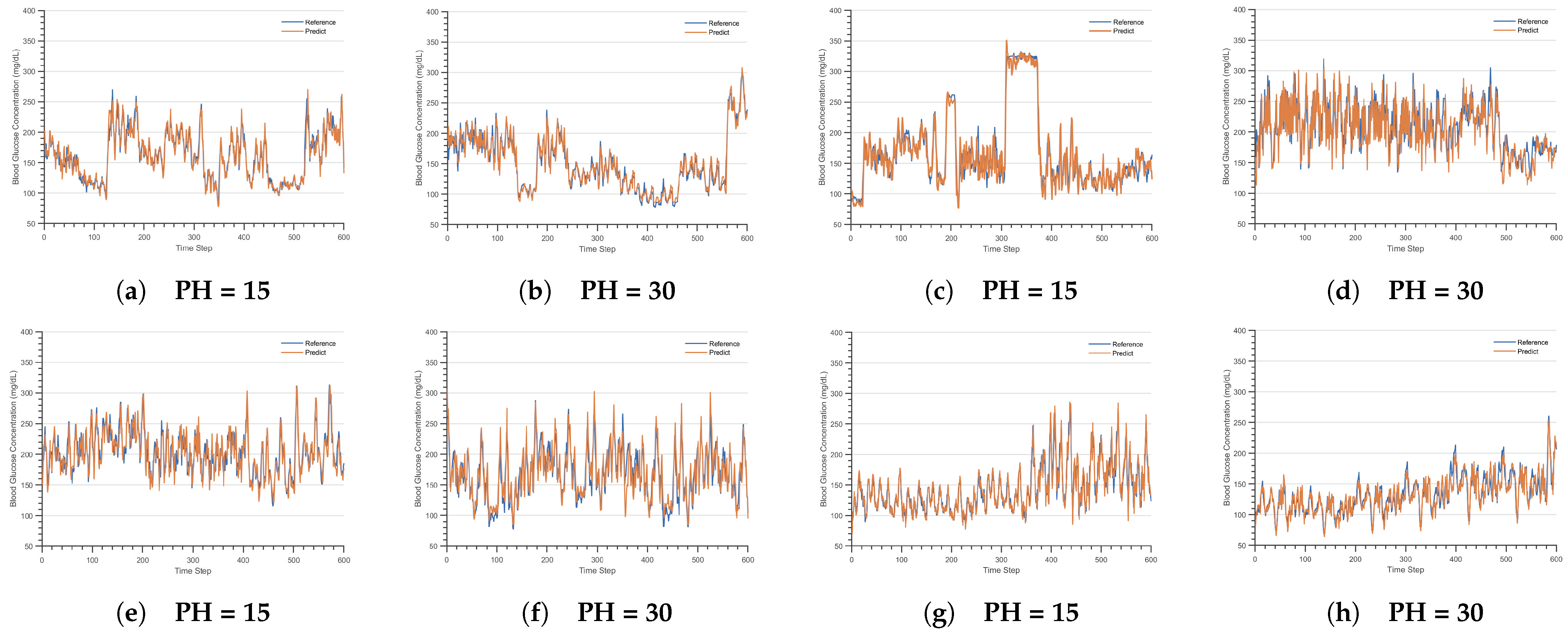
4.2.4. Results and Analysis

The MAE and RMSE outcomes from experiments conducted on a per-patient basis are detailed in

Table 1. The performance of multivariate blood glucose prediction on the D1NAMO dataset at various PH values, as measured by MAE and RMSE.

	15-min PH		30-min PH		60-min PH		120-min PH		180-min PH
Pt	MAE	RMSE	MAE	RMSE	MAE	RMSE	MAE	RMSE	MAE	RMSE
01	0.020	0.033	0.023	0.038	0.029	0.049	0.044	0.076	0.055	0.095
02	0.030	0.052	0.031	0.053	0.045	0.075	0.067	0.112	0.073	0.124
04	0.053	0.127	0.067	0.141	0.077	0.154	0.099	0.188	0.113	0.213
05	0.045	0.079	0.048	0.086	0.060	0.100	0.090	0.142	0.106	0.194
06	0.023	0.041	0.029	0.045	0.035	0.056	0.055	0.085	0.068	0.105
07	0.037	0.104	0.045	0.117	0.055	0.139	0.085	0.182	0.110	0.230
08	0.030	0.064	0.035	0.067	0.040	0.077	0.059	0.100	0.073	0.123

,

Table 2. The performance of univariate blood glucose prediction on the D1NAMO dataset at various PH values, as measured by MAE and RMSE.

	15-min PH		30-min PH		60-min PH		120-min PH		180-min PH
Pt	MAE	RMSE	MAE	RMSE	MAE	RMSE	MAE	RMSE	MAE	RMSE
01	0.027	0.036	0.036	0.050	0.060	0.089	0.113	0.148	0.128	0.183
02	0.021	0.036	0.031	0.050	0.073	0.115	0.133	0.203	0.170	0.248
04	0.033	0.046	0.038	0.054	0.092	0.129	0.137	0.175	0.161	0.194
05	0.051	0.068	0.068	0.088	0.113	0.153	0.248	0.292	0.264	0.327
06	0.013	0.018	0.034	0.048	0.039	0.056	0.075	0.100	0.111	0.134
07	0.031	0.035	0.026	0.037	0.044	0.062	0.076	0.101	0.109	0.132
08	0.030	0.041	0.031	0.041	0.081	0.101	0.121	0.145	0.161	0.184

,

Table 3. The performance of univariate blood glucose prediction on the DirecNet dataset at various PH values, as measured by MAE and RMSE.

	15-min PH		30-min PH		60-min PH		120-min PH		180-min PH
Pt	MAE	RMSE	MAE	RMSE	MAE	RMSE	MAE	RMSE	MAE	RMSE
01	0.072	0.106	0.093	0.140	0.119	0.169	0.172	0.223	0.222	0.272
02	0.101	0.152	0.126	0.176	0.185	0.236	0.273	0.337	0.277	0.334
03	0.052	0.075	0.064	0.091	0.072	0.108	0.086	0.118	0.105	0.129
04	0.071	0.086	0.070	0.092	0.105	0.144	0.165	0.214	0.284	0.328
05	0.028	0.039	0.030	0.042	0.037	0.052	0.063	0.078	0.077	0.093
06	0.050	0.069	0.050	0.071	0.081	0.109	0.124	0.156	0.117	0.145
07	0.065	0.120	0.104	0.177	0.171	0.280	0.196	0.279	0.187	0.268
08	0.040	0.052	0.054	0.068	0.079	0.101	0.118	0.149	0.147	0.186
09	0.057	0.082	0.066	0.097	0.127	0.168	0.151	0.204	0.159	0.215

and

Table 4. The performance of univariate blood glucose prediction on the T1DExchange dataset at various PH values, as measured by MAE and RMSE.

	15-min PH		30-min PH		60-min PH		120-min PH		180-min PH
Pt	MAE	RMSE	MAE	RMSE	MAE	RMSE	MAE	RMSE	MAE	RMSE
01	0.024	0.038	0.032	0.053	0.048	0.091	0.076	0.125	0.087	0.150
02	0.021	0.028	0.036	0.050	0.062	0.085	0.072	0.100	0.068	0.083
03	0.034	0.055	0.038	0.056	0.050	0.067	0.078	0.098	0.089	0.110
04	0.078	0.094	0.096	0.122	0.174	0.223	0.303	0.365	0.243	0.302
05	0.045	0.063	0.060	0.084	0.094	0.123	0.178	0.222	0.190	0.232
06	0.018	0.024	0.024	0.033	0.050	0.061	0.124	0.156	0.185	0.231
07	0.036	0.048	0.051	0.069	0.092	0.124	0.148	0.191	0.189	0.234
08	0.022	0.028	0.041	0.049	0.055	0.071	0.091	0.112	0.080	0.101
09	0.037	0.054	0.058	0.084	0.092	0.126	0.134	0.175	0.115	0.149

, with the Prediction Horizon (PH) categorized into intervals of 15, 30, 60, 120, and 180 min. For Table 1 and Table 2, Pt 03 and Pt 09 were excluded from the analysis due to their limited blood glucose data in the D1NAMO dataset, and the model was trained on data from the remaining seven patients. For Table 3 and Table 4, the model was trained using data from 9 patients in the DireNet dataset and the T1DExchange dataset, respectively.

Our model demonstrated robust performance in most patients, particularly at the 15 min PH, which outperformed other forecasting intervals. In Table 1, compared to other patients, Pt 01 achieves the best performance across all five prediction horizons; in Table 2, Pt 06 and Pt 07 exhibit similar efficacy. In Table 3, Pt 05 shows notable efficacy; in Table 4, Pt 06 shows remarkable performance in short-term predictions within 1 h, while for long-term predictions beyond 2 h, Pt 01, Pt 02, and Pt 03 also perform well. Our model achieved good results in personalized blood glucose predictions across all three datasets. The variability in predictive accuracy among patients may be attributed to several factors: in D1NAMO, Pt 05 had incomplete blood glucose data; in DirecNet, Pt 02 underwent frequent, abrupt fluctuations in blood glucose levels, particularly during periods of elevation, leading to multiple trend reversals that diminished the predictive accuracy. In T1DExchange, Pt 04 had unusually large differences between peak and trough blood glucose levels, a situation not common in other patients, which caused the model’s performance to decline as it learned new data.

Table 5. D1NAMO multivariate blood glucose prediction results.

Methods	Ours		HDMixer		Pathformer		Informer		Crossformer		Koopa
Metric	MAE	RMSE	MAE	RMSE	MAE	RMSE	MAE	RMSE	MAE	RMSE	MAE	RMSE
15	0.020	0.033	0.134	0.196	0.206	0.274	0.715	1.160	0.216	0.564	0.075	0.146
30	0.023	0.038	0.173	0.257	0.278	0.395	0.786	1.259	0.277	0.603	0.129	0.235
60	0.029	0.049	0.262	0.391	0.363	0.505	0.792	1.341	0.378	0.749	0.230	0.384
120	0.044	0.076	0.403	0.561	0.498	0.661	0.897	1.439	0.437	0.844	0.367	0.526
180	0.055	0.095	0.472	0.578	0.530	0.695	0.924	1.461	0.577	1.059	0.467	0.649
Methods	TimesNet		iTransformer		MSGNet		SOFTS		Reformer		PatchTST
Metric	MAE	RMSE	MAE	RMSE	MAE	RMSE	MAE	RMSE	MAE	RMSE	MAE	RMSE
15	0.117	0.277	0.058	0.111	0.120	0.273	0.082	0.125	0.664	1.102	0.053	0.101
30	0.130	0.291	0.103	0.171	0.127	0.283	0.130	0.201	0.706	1.190	0.097	0.161
60	0.147	0.319	0.196	0.318	0.150	0.318	0.214	0.331	0.799	1.363	0.190	0.297
120	0.177	0.374	0.355	0.512	0.180	0.359	0.357	0.499	0.865	1.422	0.329	0.468
180	0.202	0.419	0.460	0.617	0.196	0.387	0.436	0.573	0.884	1.449	0.419	0.556
Methods	FEDformer		Autoformer		DLinear		Fredformer		MTGNN		TimeGNN
Metric	MAE	RMSE	MAE	RMSE	MAE	RMSE	MAE	RMSE	MAE	RMSE	MAE	RMSE
15	0.162	0.339	0.263	0.396	0.144	0.264	0.117	0.176	2.355	3.814	3.497	4.776
30	0.180	0.356	0.270	0.421	0.191	0.332	0.160	0.242	2.733	4.161	3.662	4.935
60	0.177	0.377	0.251	0.428	0.244	0.421	0.265	0.390	3.315	4.684	3.872	5.220
120	0.174	0.388	0.244	0.435	0.348	0.595	0.405	0.554	3.778	5.138	3.879	5.262
180	0.200	0.423	0.276	0.486	0.433	0.739	0.352	0.445	3.833	4.893	3.858	4.921

illustrates the outcomes of multivariate blood glucose forecasting, where the NLAGNN excels in all 17 instances. The NLAGNN consistently outperforms the StemGNN model, underscoring the promise of the GNN architecture in time series prediction. The NLAGNN achieves notable improvements over the Transformer models; compared to iTransformer, MAE decreases by 0.200 and RMSE by 0.287.

Table 6. D1NAMO univariate blood glucose prediction results.

Methods	Ours		HDMixer		Pathformer		Informer		Crossformer		Koopa
Metric	MAE	RMSE	MAE	RMSE	MAE	RMSE	MAE	RMSE	MAE	RMSE	MAE	RMSE
15	0.027	0.036	0.132	0.197	0.187	0.268	0.570	0.715	0.158	0.234	0.087	0.176
30	0.036	0.050	0.182	0.274	0.289	0.401	0.73	0.895	0.199	0.298	0.158	0.330
60	0.060	0.089	0.259	0.384	0.348	0.487	0.907	1.127	0.331	0.462	0.255	0.436
120	0.113	0.148	0.443	0.542	0.483	0.641	1.332	1.685	0.555	0.726	0.429	0.638
180	0.128	0.183	0.470	0.565	0.525	0.685	1.376	1.668	0.813	1.005	0.515	0.696
Methods	TimesNet		iTransformer		MSGNet		SOFTS		Reformer		PatchTST
Metric	MAE	RMSE	MAE	RMSE	MAE	RMSE	MAE	RMSE	MAE	RMSE	MAE	RMSE
15	0.057	0.118	0.058	0.111	0.060	0.106	0.082	0.125	0.573	0.713	0.053	0.101
30	0.102	0.189	0.103	0.171	0.103	0.171	0.130	0.201	0.627	0.797	0.097	0.161
60	0.193	0.316	0.196	0.318	0.194	0.309	0.213	0.331	0.823	1.048	0.190	0.297
120	0.349	0.534	0.355	0.512	0.339	0.493	0.356	0.499	0.956	1.172	0.329	0.468
180	0.436	0.633	0.460	0.617	0.427	0.591	0.436	0.573	1.176	1.438	0.419	0.556
Methods	FEDformer		Autoformer		DLinear		Fredformer		MTGNN		TimeGNN
Metric	MAE	RMSE	MAE	RMSE	MAE	RMSE	MAE	RMSE	MAE	RMSE	MAE	RMSE
15	0.242	0.388	0.320	0.470	0.217	0.278	0.109	0.162	0.522	0.781	2.475	3.249
30	0.272	0.414	0.394	0.567	0.267	0.345	0.165	0.247	1.157	1.578	3.524	4.572
60	0.316	0.494	0.376	0.554	0.382	0.485	0.284	0.418	2.212	2.790	4.675	5.968
120	0.410	0.618	0.419	0.605	0.602	0.760	0.403	0.561	3.793	4.712	5.435	6.867
180	0.318	0.596	0.403	0.613	0.772	0.967	0.370	0.454	4.108	5.003	5.249	6.688

,

Table 7. DirecNet univariate blood glucose prediction results.

Methods	Ours		HDMixer		Pathformer		Informer		Crossformer		Koopa
Metric	MAE	RMSE	MAE	RMSE	MAE	RMSE	MAE	RMSE	MAE	RMSE	MAE	RMSE
15	0.072	0.106	0.412	0.583	0.468	0.678	0.485	0.660	0.206	0.325	0.347	0.604
30	0.093	0.140	0.550	0.732	0.606	0.829	0.675	0.933	0.335	0.487	0.492	0.763
60	0.119	0.169	0.664	0.876	0.781	1.018	0.972	1.254	0.578	0.801	0.729	0.943
120	0.172	0.223	0.815	1.079	0.942	1.214	1.204	1.540	0.745	0.995	0.830	1.138
180	0.222	0.272	0.950	1.244	1.121	1.420	1.307	1.669	0.939	1.228	0.954	1.261
Methods	TimesNet		iTransformer		MSGNet		SOFTS		Reformer		PatchTST
Metric	MAE	RMSE	MAE	RMSE	MAE	RMSE	MAE	RMSE	MAE	RMSE	MAE	RMSE
15	0.310	0.486	0.318	0.479	0.297	0.480	0.315	0.503	0.518	0.698	0.273	0.462
30	0.420	0.657	0.393	0.611	0.428	0.618	0.426	0.645	0.657	0.864	0.399	0.594
60	0.597	0.807	0.598	0.804	0.591	0.795	0.621	0.858	0.901	1.154	0.546	0.767
120	0.740	1.031	0.724	0.998	0.739	1.020	0.796	1.055	1.140	1.451	0.725	0.997
180	0.888	1.207	0.879	1.183	0.905	1.208	0.956	1.240	1.098	1.400	0.868	1.182
Methods	FEDformer		Autoformer		DLinear		Fredformer		MTGNN		TimeGNN
Metric	MAE	RMSE	MAE	RMSE	MAE	RMSE	MAE	RMSE	MAE	RMSE	MAE	RMSE
15	0.577	0.755	0.498	0.676	0.364	0.494	0.208	0.287	1.068	1.514	2.892	3.737
30	0.731	0.913	0.657	0.876	0.448	0.613	0.313	0.434	1.994	2.638	3.914	5.028
60	0.848	1.061	0.904	1.143	0.579	0.790	0.519	0.675	3.166	4.035	4.689	6.028
120	0.977	1.241	1.011	1.295	0.743	1.002	0.663	0.882	4.288	5.457	5.122	6.505
180	1.029	1.303	1.074	1.361	0.837	1.112	0.837	1.074	4.666	5.954	5.143	6.582

and

Table 8. T1DExchange univariate blood glucose prediction results.

Methods	Ours		HDMixer		Pathformer		Informer		Crossformer		Koopa
Metric	MAE	RMSE	MAE	RMSE	MAE	RMSE	MAE	RMSE	MAE	RMSE	MAE	RMSE
15	0.037	0.054	0.205	0.304	0.489	0.687	0.834	1.150	0.166	0.320	0.158	0.246
30	0.058	0.084	0.288	0.431	0.555	0.782	0.852	1.159	0.274	0.453	0.252	0.385
60	0.092	0.126	0.422	0.623	0.620	0.862	0.851	1.187	0.470	0.726	0.460	0.669
120	0.134	0.175	0.605	0.883	0.727	0.999	0.886	1.212	0.645	0.973	0.653	0.930
180	0.115	0.149	0.711	1.031	0.816	1.126	0.866	1.222	0.744	1.068	0.744	1.072
Methods	TimesNet		iTransformer		MSGNet		SOFTS		Reformer		PatchTST
Metric	MAE	RMSE	MAE	RMSE	MAE	RMSE	MAE	RMSE	MAE	RMSE	MAE	RMSE
15	0.614	0.858	0.119	0.194	0.179	0.264	0.118	0.191	0.827	1.156	0.126	0.200
30	0.644	0.902	0.203	0.325	0.264	0.393	0.215	0.337	0.858	1.161	0.204	0.321
60	0.712	0.987	0.354	0.549	0.420	0.620	0.365	0.560	0.837	1.196	0.349	0.539
120	0.793	1.100	0.560	0.830	0.617	0.902	0.569	0.845	0.868	1.189	0.550	0.818
180	0.851	1.188	0.681	0.998	0.745	1.079	0.689	1.007	0.889	1.213	0.668	0.980
Methods	FEDformer		Autoformer		DLinear		Fredformer		MTGNN		TimeGNN
Metric	MAE	RMSE	MAE	RMSE	MAE	RMSE	MAE	RMSE	MAE	RMSE	MAE	RMSE
15	0.630	0.844	0.392	0.533	0.277	0.365	0.161	0.240	0.630	0.957	1.591	2.170
30	0.680	0.909	0.468	0.635	0.363	0.480	0.248	0.369	1.234	1.719	2.249	3.388
60	0.716	0.981	0.567	0.784	0.487	0.660	0.377	0.562	2.202	2.912	3.173	4.294
120	0.808	1.125	0.760	1.061	0.634	0.875	0.566	0.820	3.064	4.109	3.370	4.496
180	0.857	1.208	0.884	1.217	0.708	0.987	0.660	0.941	3.198	4.308	3.323	4.359

present the results of univariate blood sugar predictions across various datasets, where our model again secures top performance. Compared with the PatchTST model within the Patch baseline, the NLAGNN shows significant advancement, with MAE reduced by 0.183 and RMSE by 0.258. In contrast to the Koopa model based on Koopman theory, at a 15 min PH, the MAE decreases by 0.055 and the RMSE by 0.113; at a 180 min PH, the MAE decreases by 0.412 and the RMSE by 0.554. Compared to the SOFTS model, which is similarly designed for multivariate sequence tasks, the Mean Absolute Error (MAE) decreases by 0.081, and the Root Mean Squared Error (RMSE) decreases by 0.173.

In prediction tasks, the accepted error range is in the range of (0, 1]. Using the multivariate blood glucose dataset D1NAMO as an example, we compared several Transformer-based models, as shown in Table 5. The results show that the RMSE of both Informer and Reformer exceeds 1 across all prediction horizons, which is unacceptable for this task. Additionally, their MAE results also demonstrate poor performance in short-term prediction horizons. This may be because these models are designed for ultra-long time series analysis, such as annual weather or large-scale traffic data. However, blood glucose data from diabetes patients are collected through external devices, such as wearable devices or continuous glucose monitoring systems (CGMs). These devices are typically not worn for extended periods, and patients may stop testing during daily activities, leading to discontinuous data collection. Furthermore, Reformer is better suited for text or audio tasks, while Informer is designed for other specialized tasks.

Autoformer employs an automated search strategy to identify the optimal Transformer architecture, reducing the need for manual adjustments. However, since Autoformer is primarily designed for visual recognition tasks, its performance is inadequate for time-series prediction. FEDformer integrates a seasonal-trend decomposition method, enabling detailed analysis of time-series structures. However, blood glucose data are assessed in real time, not seasonally. As a result, FEDformer’s seasonal-trend decomposition method shows no advantages in the D1NAMO dataset, leading to diminished performance. Crossformer employs a two-stage attention mechanism to manage temporal and dimensional dependencies separately, utilizing multi-scale information to improve performance. Notably, this approach does not account for data sparsity. Due to the highly sparse distribution of insulin data, the two-stage attention mechanism mishandles data sparsity, increasing long-term prediction errors. iTransformer, with its simple structure, efficiently handles time-series data. However, it is overly sensitive to clear trends and struggles to detect sudden data fluctuations, reducing its effectiveness on the blood glucose dataset. Similarly, Pathformer enhances predictive capabilities through adaptive paths, but this comes at the cost of increased computational complexity. It also suffers from typical spatio-temporal separation issues. Specifically, TimesNet transforms one-dimensional time series into a two-dimensional structure, enabling the model to capture both intra-period and inter-period variations. Fredformer models in the frequency domain, reducing the model’s bias toward low-frequency features and enabling balanced learning across all frequency bands. Among these models, Fredformer’s performance at PH = 180 was second only to the NLAGNN’s, outperforming all other models.

HDMixer is specifically designed for insulin variables, carefully addressing the sparsity of insulin data and capturing features closely linked to blood glucose. However, its focus on other variables is insufficient to significantly improve performance. DLinear is primarily designed for simple linear patterns, whereas Koopa is overly sensitive to noise and outliers. The STAR module in SOFTS is tailored to specific datasets. PatchTST divides the time series into small patches and improves the model’s generalization through an independent channel design, achieving the second-best performance in most cases within this dataset. Finally, an examination of the prediction results of GNN-based models, including MSGNet, MTGNN, and TimeGNN, revealed that MTGNN is specifically designed for multivariate traffic flow prediction. TimeGNN captures sequence pattern evolution by learning dynamic time-graph representations; however, it struggles with nonlinear features and complex dynamics. MSGNet, inspired by PatchTST’s design, efficiently extracts significant cyclical patterns in the data via frequency-domain analysis. For blood glucose data, MSGNet’s dependence on strong periodicity resulted in average performance on our dataset.

Although our model demonstrates competitive results in blood glucose prediction, TimeGNN offers greater advantages in feature extraction for data from dynamic environments. For ultra-long multivariate sequence prediction, Transformers, leveraging self-attention, positional encoding, and parallel computing, can achieve superior predictive performance. It is crucial to recognize that different models excel in specific environments.

Additionally, the performance of various models is presented in

Table 9. Performance comparison of the D1NAMO dataset.

Method	Ours	Fredformer	SOFTS	Autoformer	FEDformer	DLinear	Crossformer	iTransformer	Informer
Params (M)	0.66	8.73	1.71	1.46	1.46	7.80 × ${10}^{-5}$	6.61	0.80	1.66
AvgIT (ms)	9.20	0.02	0.05	4.74	24.00	1.16	4.78	1.02	5.50
FLOPs (M)	59.50	1442.07	17.13	8.76	8.77	1.76 × ${10}^{-4}$	30.49	8.07	9.40
Method	Koopa	PatchTST	Reformer	TimesNet	TimeGNN	MTGNN	HDMixer	Pathformer	MSGNet
Params (M)	0.19	0.80	0.67	286.05	0.02	0.33	0.02	0.54	0.98
AvgIT (ms)	5.41	0.99	0.84	25.20	8.97	9.21	8.82 × ${10}^{-4}$	1.85	9.47
FLOPs (M)	0.91	3.99	11.00	6223.16	3.21	45.84	1.67	7.20	55.45

. By comparing three metrics—Params, Average Inference Time (AvgIT), and floating-point operations (FLOPs)—we found that the NLAGNN’s superior predictive performance is attributed to its three components: NFGO, Dynamic Subgraph Partitioning (DSG), and GAA. However, this performance comes at the cost of a larger model size and longer inference time, allowing for it to capture branch feature information at different scales. Although we considered the complexity of the graph data structure and introduced Fourier operators to reduce time complexity, the model size did not decrease. The FLOPs reached 59.50 M, and the AvgIT was 9.2 ms, both higher than in most other models.

Since the model will eventually be deployed on devices with performance constraints, we can compress it in the following ways: shallow feature maps, such as those derived from ablation studies, can serve as supervision signals for smaller models to approximate more complex ones. In population-level blood glucose trend prediction, post-training quantization is applied, eliminating the need for model retraining. Additionally, kernel importance is assessed by analyzing weight activation and gradient information. The least impactful kernels are pruned, and the model is then retrained.

To further improve the model’s performance in real-time clinical scenarios, we consider parallelization strategies and edge computing. Data can be partitioned into smaller batches near the source and assigned to different units for processing, effectively reducing latency. Based on the earlier ablation studies, different parts of the model and training tasks can be offloaded to edge servers and executed by distinct processing units. This hybrid architecture optimizes medical resource use and enables efficient task allocation between mobile devices and edge servers based on real-time needs, maximizing resource utilization in healthcare.

4.3. Ablation Study

To assess the efficacy of the components of the NLAGNN, an ablation study was performed on representative patients from each dataset, concentrating on the dynamic segmentation mechanism and the layer aggregation strategy. The findings from the ablation study indicate that the superior predictive accuracy of our approach stems not from any isolated element, but from the synergistic integration of all its components. For clarity, the multivariate and univariate data from the D1NAMO dataset are referenced as 1 and 2, respectively.

Table 10. Model ablation study of different components at PH = 15 in various datasets.

Dataset	D1NAMO-1		D1NAMO-2		DirecNet		T1DExchange
Metric	MAE	RMSE	MAE	RMSE	MAE	RMSE	MAE	RMSE
Baseline	0.083	0.149	0.070	0.093	0.199	0.230	0.040	0.060
W/O SSE	0.019	0.030	0.031	0.043	0.079	0.117	0.021	0.033
W/O FCK	0.019	0.032	0.032	0.045	0.080	0.119	0.037	0.043
W/O GAA	0.019	0.030	0.027	0.036	0.077	0.119	0.026	0.039
NLAGNN	0.018	0.029	0.025	0.034	0.072	0.106	0.018	0.024

presents the findings of our ablation study, detailing the impacts of W/O SSE, W/O FCK, and W/O GAA—scenarios in the absence of subgraph semantic enhancement, feature combination kernels, and graph aggregation strategies, respectively. The exclusion of any component results in diminished model accuracy. The ablation experiment results show that across all three datasets, the baseline model, which utilized only the nonlinear Fourier graph neural operator, exhibited the poorest performance. In contrast, the model incorporating subgraph semantic enhancement (SSE), multi-scale fusion convolution (FCK), and layer aggregation (AGG) exhibited substantial performance improvements. Specifically, in the DINAMO-1 multivariate dataset, our NLAGNN model reduced MAE by 0.065 and RMSE by 0.120 compared to the baseline. These improvements were primarily driven by the combined effects of SSE, FCK, and AGG. When the SSE component was blocked, MAE decreased by 0.064, and RMSE decreased by 0.119. Additionally, the combination of SSE and GAA reduced MAE by 0.064 and RMSE by 0.117. Blocking the GAA component alone resulted in a reduction in MAE by 0.064 and RMSE by 0.119. Similar performance improvements were observed across the remaining univariate datasets, with the T1DExchange dataset showing the greatest gains—MAE decreased by 0.022, and RMSE decreased by 0.036. In the DINAMO-2 and DirecNet datasets, the combination of SSE and FCK contributed to notable performance gains, reducing MAE by 0.122 and RMSE by 0.111.

Experimental data confirm that the SSE component effectively addresses the issue of unclear strong and weak variable correlations persisting after node nonlinearization. It reduces irrelevant noise, highlights strongly correlated features, and sharpens the model’s focus on key variables such as insulin. Additionally, the FCK component activates both strong and weak correlations, amplifying inter-variable relationships while minimizing the impact of weak correlations and noise on model performance. Furthermore, the GAA component’s multi-dimensional graph layer aggregation allows the model to distinguish between variables like body posture, breathing rate, and ECG in relation to blood glucose while identifying intra-variable similarities. This enhances the model’s ability to detect and capture comprehensive similarity features across variables.

To visually assess the accuracy of blood glucose predictions, Clarke Error Grid Analysis (EGA) was employed, which evaluates the clinical significance of discrepancies between actual and projected blood glucose levels. The horizontal axis represents the reference values of blood glucose, while the vertical axis denotes the predicted values. The EGA is divided into five distinct zones, each with unique medical implications:

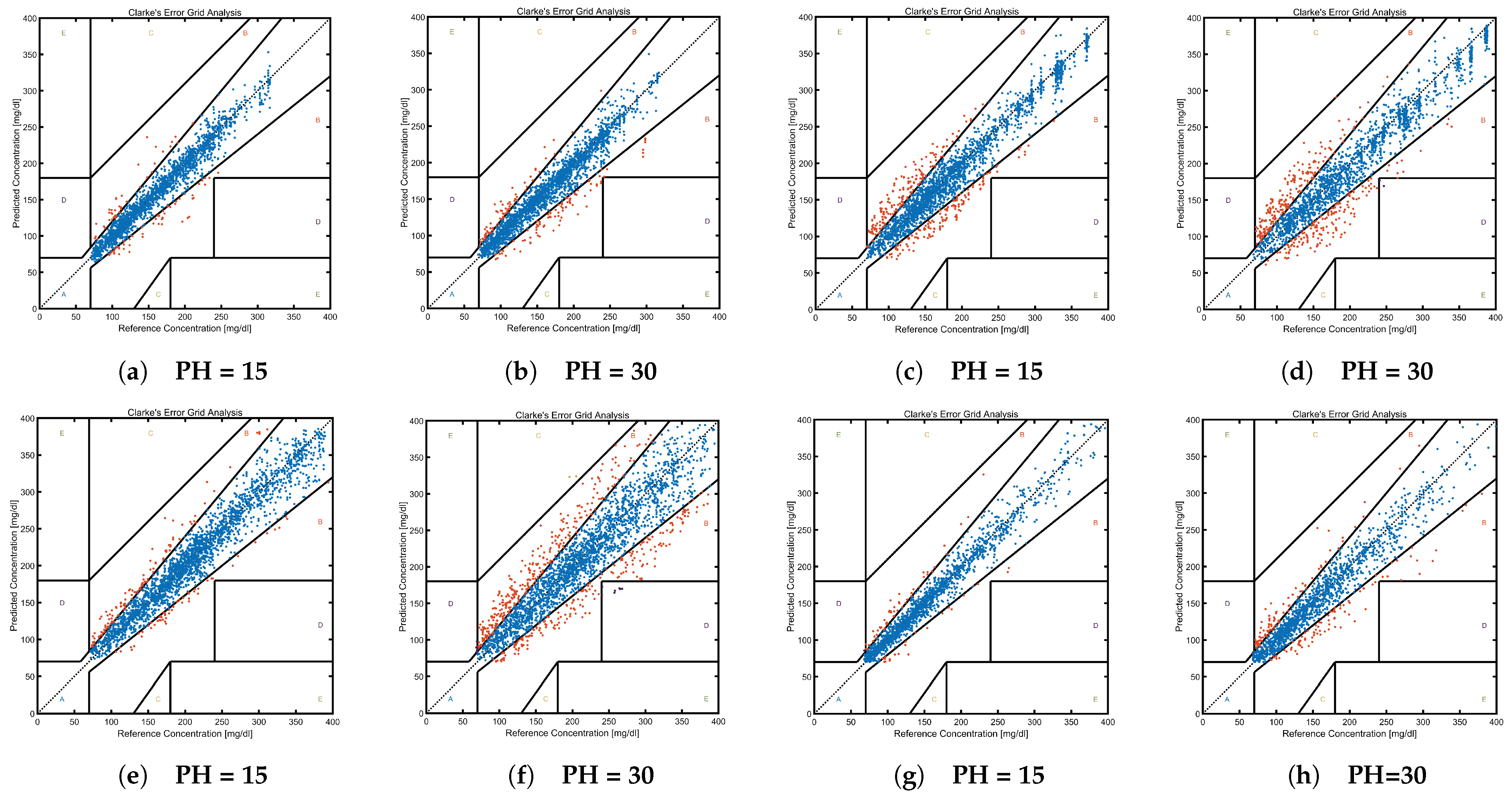
• Zone A (Acceptable Zone): Predicted values are within ±20% of the reference values or within ±15 mg/dL during hypoglycemia (<70 mg/dL).
• Zone B (Benign Error Zone): Predicted values, though deviating from the reference values, do not significantly influence patient management.
• Zones C, D, and E: These zones indicate critical errors between predicted and reference values, warranting immediate clinical attention.

Clarke EGA provides a graphical depiction, aiding healthcare professionals and researchers in gauging the potential clinical ramifications of predictive inaccuracies, thereby ensuring that predictions are both precise and clinically meaningful.

Figure 2 presents the Clarke EGA for different datasets at varying prediction horizons. Pairs (a) and (b), (c) and (d), and (e) and (f) correspond to the blood glucose prediction distributions in the D1NAMO-1, D1NAMO-2, DirecNet, and T1DExchange datasets, respectively. Synthesizing these results with

Table 11. Distribution of Clarke Error grid analysis zones.

Dataset	PH	A + B	C + D + E
D1NAMO-1	15	87.48 + 12.52%	0
	30	83.62 + 16.29%	00.09%
D1NAMO-2	15	96.01 + 03.99%	0
	30	93.27 + 06.73%	0
DirecNet	15	93.43 + 06.57%	0
	30	80.35 + 19.09%	00.56%
T1DExchange	15	95.80 + 04.14%	00.06%
	30	88.97 + 10.90%	00.13%

reveals that the combined proportion of Zones A and B exceeds 99% across datasets, whereas Zones C, D, and E constitute less than 1%. An incremental PH value induces a minor transition of predictions from the acceptable zone to the benign error zone, with the majority of predictions residing within clinically safe zones and minimal in others. This outcome is predominantly attributed to the Graph Aggregation Attention (GAA) component, which integrates the features of highly correlated variables at the graph level. This aggregation empowers our method to maintain a 99% safe prediction rate within the initial 30 min of the PH.

Figure 3 illustrates the actual and predicted blood glucose trajectories for D1NAMO-1, D1NAMO-2, DirecNet, and T1DExchange datasets at different prediction horizons. Specifically, subgraphs (a) and (b) correspond to the D1NAMO-1 dataset, (c) and (d) to D1NAMO-2, (e) and (f) to DirecNet, and (g) and (h) to T1DExchange. The graphical analysis reveals that the predicted trajectories closely match the actual trajectories, with a particularly strong alignment observed at a prediction horizon of 15 min, exceeding the accuracy at a 30 min prediction horizon. Overall, the short-term predictions exhibit a notably higher accuracy.

5. Discussion

The technical process of the NLAGNN model in a personalized treatment plan integration involves a series of complex data processing and deep learning operations. First, data on the patient’s lifestyle, dietary habits, and activity frequency are collected, and preprocessing techniques are applied to clean the raw data, ensuring data quality. Next, feature extraction algorithms are employed to identify key variables closely related to blood glucose, providing the model with high-quality training data. During training, the NLAGNN model relies on several key components to effectively utilize multivariate blood glucose data. By training on extensive historical blood glucose data, the model learns complex glucose variations and inter-variable relationships, allowing it to predict future trends.

In the diabetes early warning system, the model analyzes patients’ physiological data patterns and behavioral tendencies using deep learning algorithms, enabling it to predict impending hyperglycemic or hypoglycemic events. The model leverages its advanced time-series analysis capabilities to effectively detect abnormal blood glucose fluctuations, promptly issuing warning signals to patients and healthcare professionals. Integrated with medical emergency response systems, the model automatically notifies in-hospital emergency services during severe hyperglycemic or hypoglycemic events, ensuring patients receive timely medical care. This warning mechanism not only provides the medical team with a valuable time window but also enhances patients’ ability to manage blood glucose, enabling both to take swift action. The model’s real-time monitoring and predictive capabilities, seamlessly integrated with existing healthcare information systems, create a comprehensive early warning and response network, significantly improving the quality of life and safety for diabetic patients.

The surge of clinical data has driven the development of Clinical Decision Support Systems (CDSS), gradually transforming the operational environment, work practices, and thought processes in healthcare. Medical knowledge bases, which form the foundation of CDSS, store expert diagnostic knowledge, medical facts, and diagnostic rules. When embedded in the system, the model can utilize initial data from diabetic patients in the global database to select corresponding variable rules from the medical knowledge base. It then executes these rules to optimize the database and, through continuous reasoning, reaches final conclusions. The model provides physicians with detailed explanations of the relationships between multivariate data, aiding healthcare professionals in making more informed decisions. Similarly, the model can be integrated into wearable devices and telemedicine platforms. Wearable devices are designed to collect patients’ physiological data continuously. Using non-invasive sensors, these devices effectively monitor vital signs such as respiration rate, heart rate, and blood glucose, and they upload the data to a cloud platform. The model then analyzes and processes the data, generating accurate blood glucose predictions. Telemedicine platforms can access the analyzed data through wearable devices, enabling real-time monitoring of patients’ health and providing consultations or interventions as needed. This approach creates a complementary relationship between wearable devices and telemedicine platforms, integrating both monitoring and early warning functions, offering patients comprehensive diabetes management.

The experimental results show that our model has a strong ability to predict blood glucose levels in patients across different age groups, clearly demonstrating the importance of integrating deep learning models into rehabilitation engineering. During rehabilitation, the model monitors blood glucose responses to internal and external stimuli, such as physical activity and dietary changes. This real-time monitoring allows healthcare providers to adjust the rehabilitation plan as needed, ensuring optimal blood glucose management throughout the process. By tracking post-intervention changes, the model provides feedback to patients, guiding them toward sustainable lifestyle changes. This approach improves patient compliance, contributing to the overall success of the rehabilitation plan. In population health management, the model’s application shifts from personalized care to population-level health predictions. Continuous Glucose Monitoring (CGM) systems collect blood glucose data from large patient cohorts, supplying the model with extensive real-world data. After processing and analysis, the deep learning algorithm identifies patterns and predicts population-level blood glucose levels. By analyzing trends in regional blood glucose levels to forecast resource needs and inform preventive healthcare planning, the significance of these predictions for the healthcare system becomes clear.

Finally, when integrating the model into healthcare, strict regulations must be enforced, and the model’s safety in clinical applications must be ensured. To maintain the model’s safety and stability in practical use, collaboration with regulatory bodies like the NMPA, EMA, and FDA is necessary to validate the model and ensure it meets medical device efficacy and safety standards. This collaboration is key to mitigating risks associated with the model. Ensuring global regulatory consistency is another crucial step, requiring a comprehensive evaluation of the model and its application scenarios to comply with varying regulatory systems across countries and regions. This includes adherence to medical device regulations, patient data protection laws, and AI ethical guidelines, with full transparency to ensure the model’s decision-making is interpretable, addressing any arising issues.

6. Conclusions

This study leveraged deep learning techniques to predict blood glucose levels in diabetes patients across various time periods. We propose a novel GNN-based predictor (NLAGNN) as an effective multivariate method for blood glucose prediction in time series forecasting. The model consists of three key components to enhance prediction accuracy for diabetes patients. First, we model the raw data as a hypergraph, preserving the original temporal and spatial correlations, which improves early blood glucose prediction and better aligns with clinical diagnosis. Second, the Nonlinear Fourier Graph Neural Operator (NFGO) enables a nonlinear representation of all variable nodes, activating strongly or weakly correlated variable features while reducing meaningless noise and lowering computational complexity. The Dynamic Subgraph Division (DSG) component processes the reassembled feature graph following node enhancement and subgraph concatenation, extracting strongly correlated variable features to improve feature distinguishability. This enhances the model’s ability to recognize diverse features and learn comprehensive information from correlated variables. Finally, features extracted at both the node and subgraph levels are aggregated through multi-branch aggregation, including intra-variable and inter-variable aggregation. This module effectively uses multi-scale channels to integrate information from different branches, allowing for accurate predictions based on varying feature strengths. Furthermore, Clarke Error Grid Analysis (CEGA) was used to visualize prediction results during decision-making, validating the model’s credibility and accuracy in diabetes diagnosis and confirming the effectiveness of the proposed components. Compared to various existing methods, extensive experimental results demonstrate the effectiveness of the NLAGNN on three public datasets, exhibiting competitive performance. The results show that DL models hold substantial promise for predicting blood glucose levels. From this, we can infer that in the medical field, our model can analyze patient data, such as daily activities and dietary habits, to offer personalized blood glucose management. This helps healthcare professionals adjust treatment plans promptly and reduce hyperglycemic and hypoglycemic events. Additionally, it can be integrated into mobile health apps and clinical decision support systems, providing real-time decision support to both doctors and patients, enhancing self-management, and easing the strain on healthcare resources.

References

1. International Diabetes Federation, 10th ed.; IDF Diabetes Atlas: Brussels, Belgium, 2021; Available online: https://www.diabetesatlas.org (accessed on 12 March 2023).
2. Dunya, T.; Shaw, J.E.; Magliano, D.J. The burden and risks of emerging complications of diabetes mellitus. Nat. Rev. Endocrinol. 2022, 18, 525–539. [Google Scholar]
3. Rodriguez Leon, C.; Banos, O.; Fernandez Mora, O.; Martinez Bedmar, A.; Rufo Jimenez, F.; Villalonga, C. Advances in Computational Intelligence. In Proceedings of the 17th International Work-Conference on Artificial Neural Networks, Ponta Delgada, Portugal, 19–21 June 2023; Springer: Cham, Switzerland, 2023; pp. 563–573. [Google Scholar]
4. Rubin-Falcone, H.; Lee, J.; Wiens, J. Forecasting with sparse but informative variables: A case study in predicting blood glucose. In Proceedings of the AAAI Conference on Artificial Intelligence, Washington, DC, USA, 7–14 February 2023; pp. 9650–9657. [Google Scholar]
5. Annuzzi, G.; Apicella, A.; Arpaia, P.; Bozzetto, L.; Criscuolo, S.; De Benedetto, E.; Pesola, M.; Prevete, R. Exploring Nutritional Influence on Blood Glucose Forecasting for Type 1 Diabetes Using Explainable AI. IEEE J. Biomed. Health Inform. 2024, 28, 3123–3133. [Google Scholar] [CrossRef]
6. Della Cioppa, A.; De Falco, I.; Koutny, T.; Scafuri, U.; Ubl, M.; Tarantino, E. Reducing high-risk glucose forecasting errors by evolving interpretable models for Type 1 diabetes. ASC 2023, 134, 110012. [Google Scholar] [CrossRef]
7. Shuvo, M.M.H.; Islam, S.K. Deep Multitask Learning by Stacked Long Short-Term Memory for Predicting Personalized Blood Glucose Concentration. IEEE J. Biomed. Health 2023, 27, 1612–1623. [Google Scholar] [CrossRef] [PubMed]
8. Aliberti, A.; Pupillo, I.; Terna, S.; Macii, E.; Di Cataldo, S.; Patti, E.; Acquaviva, A. A Multi-Patient Data-Driven Approach to Blood Glucose Prediction. IEEE Access 2019, 7, 69311–69325. [Google Scholar] [CrossRef]
9. Langarica, S.; Rodriguez-Fernandez, M.; Doyle, F.J., III; Núñez, F. A probabilistic approach to blood glucose prediction in type 1 diabetes under meal uncertainties. IEEE J. Biomed. Health Inform. 2023, 27, 5054–5065. [Google Scholar] [CrossRef]
10. Zhu, T.; Li, K.; Herrero, P.; Georgiou, P. Personalized blood glucose prediction for type 1 diabetes using evidential deep learning and meta-learning. IEEE Trans. Biomed. Eng. 2022, 70, 193–204. [Google Scholar] [CrossRef] [PubMed]
11. Butunoi, B.-P.; Stolojescu-Crisan, C.; Negru, V. Short-term glucose prediction in Type 1 Diabetes. Procedia Comput. Sci. 2024, 238, 41–48. [Google Scholar] [CrossRef]
12. Martinsson, J.; Schliep, A.; Eliasson, B.; Mogren, O. Blood glucose prediction with variance estimation using recurrent neural networks. J. Healthc. Inform. Res. 2020, 4, 1–18. [Google Scholar] [CrossRef]
13. Khanam, J.J.; Foo, S. A comparison of machine learning algorithms for diabetes prediction. ICT Express 2021, 7, 432–439. [Google Scholar] [CrossRef]
14. Ahmed, U.; Issa, G.F.; Khan, M.A.; Aftab, S.; Khan, M.F.; Said, R.A.; Ghazal, T.M.; Ahmad, M. Prediction of diabetes empowered with fused machine learning. IEEE Access 2022, 10, 8529–8538. [Google Scholar] [CrossRef]
15. Wang, S.; Chen, Y.; Cui, Z.; Lin, L.; Zong, Y. Diabetes Risk Analysis Based on Machine Learning LASSO Regression Model. J. Theory Pract. Eng. Sci. 2024, 4, 58–64. [Google Scholar]
16. Feng, Y.; You, H.; Zhang, Z.; Ji, R.; Gao, Y. Hypergraph neural networks. Proc. AAAI Conf. Artif. Intell. 2019, 33, 3558–3565. [Google Scholar] [CrossRef]
17. Diabetes Research in Children Network Study Group. The accuracy of the CGMS™ in children with type 1 diabetes: Results of the Diabetes Research in Children Network (DirecNet) accuracy study. Diabetes Technol. Ther. 2003, 5, 781–789. [Google Scholar] [CrossRef]
18. Dubosson, F.; Ranvier, J.-E.; Bromuri, S.; Calbimonte, J.-P.; Ruiz, J.; Schumacher, M. The open D1NAMO dataset: A multi-modal dataset for research on non-invasive type 1 diabetes management. Inform. Med. Unlocked 2018, 13, 92–100. [Google Scholar] [CrossRef]
19. Rickels, M.R.; DuBose, S.N.; Toschi, E.; Beck, R.W.; Verdejo, A.S.; Wolpert, H.; Cummins, M.J.; Newswanger, B.; Riddell, M.C.; T1D Exchange Mini-Dose Glucagon Exercise Study Group. Mini-Dose Glucagon as a Novel Approach to Prevent Exercise-Induced Hypoglycemia in Type 1 Diabetes. Diabetes Care 2018, 41, 1909–1916. [Google Scholar] [CrossRef] [PubMed]
20. Sirlanci, M.; Levine, M.E.; Low Wang, C.C.; Albers, D.J.; Stuart, A.M. A simple modeling framework for prediction in the human glucose–insulin system. Chaos 2023, 33, 7. [Google Scholar] [CrossRef] [PubMed]
21. Harleen, K.; Kumari, V. Predictive modelling and analytics for diabetes using a machine learning approach. Appl. Comput. Inform. 2022, 18, 90–100. [Google Scholar]
22. Khadem, H.; Nemat, H.; Elliott, J.; Benaissa, M. Blood Glucose Level Time Series Forecasting: Nested Deep Ensemble Learning Lag Fusion. Bioengineering 2023, 10, 487. [Google Scholar] [CrossRef]
23. De Bois, M.; Yacoubi, M.A.E.; Ammi, M. GLYFE: Review and benchmark of personalized glucose predictive models in type 1 diabetes. Med. Biol. Eng. Comput. 2022, 60, 1–17. [Google Scholar] [CrossRef]
24. Li, K.; Daniels, J.; Liu, C.; Herrero, P.; Georgiou, P. Convolutional Recurrent Neural Networks for Glucose Prediction. IEEE J. Biomed. Health Inform. 2020, 24, 603–613. [Google Scholar] [CrossRef] [PubMed]
25. Prendin, F.; Pavan, J.; Cappon, G.; Del Favero, S.; Sparacino, G.; Facchinetti, A. The importance of interpreting machine learning models for blood glucose prediction in diabetes: An analysis using SHAP. Sci. Rep. 2023, 13, 16865. [Google Scholar] [CrossRef] [PubMed]
26. Langarica, S.; Rodriguez-Fernandez, M.; Núñez, F.; Doyle, F., III. Meta-learning approach to personalized blood glucose prediction in type 1 diabetes. Control Eng. Pract. 2023, 135, 105498. [Google Scholar] [CrossRef]
27. Alhirmizy, S.; Qader, B. Multivariate time series forecasting with LSTM for Madrid, Spain pollution. In Proceedings of the 2019 International Conference on Computing and Information Science and Technology and Their Applications (ICCISTA), Kirkuk, Iraq, 3–5 March 2019; pp. 1–5. [Google Scholar]
28. Widiputra, H.; Mailangkay, A.; Gautama, E.J.C. Multivariate CNN-LSTM Model for Multiple Parallel Financial Time-Series Prediction. Complexity 2021, 2021, 9903518. [Google Scholar] [CrossRef]
29. Zerveas, G.; Jayaraman, S.; Patel, D.; Bhamidipaty, A.; Eickhoff, C. A transformer-based framework for multivariate time series representation learning. In Proceedings of the 27th ACM SIGKDD Conference on Knowledge Discovery and Data Mining, Singapore, 14–18 August 2021; pp. 2114–2124. [Google Scholar]
30. Yi, K.; Zhang, Q.; Fan, W.; He, H.; Hu, L.; Wang, P.; An, N.; Cao, L.; Niu, Z. FourierGNN: Rethinking multivariate time series forecasting from a pure graph perspective. arXiv 2024, arXiv:2311.06190. [Google Scholar]
31. Han, H.; Zhang, M.; Hou, M.; Zhang, F.; Wang, Z.; Chen, E.; Wang, H.; Ma, J.; Liu, Q. STGCN: A spatial-temporal aware graph learning method for POI recommendation. In Proceedings of the 2020 IEEE International Conference on Data Mining (ICDM), Sorrento, Italy, 17–20 November 2020; pp. 1052–1057. [Google Scholar]
32. Cirstea, R.-G.; Guo, C.; Yang, B. Graph Attention Recurrent Neural Networks for Correlated Time Series Forecasting–Full version. arXiv 2021, arXiv:2103.10760. [Google Scholar]
33. Zhou, Z.; Huang, Q.; Lin, G.; Yang, K.; Bai, L.; Wang, Y. Greto: Remedying dynamic graph topology-task discordance via target homophily. In Proceedings of the Eleventh International Conference on Learning Representations, Kigali, Rwanda, 1–5 May 2023. [Google Scholar]
34. Zheng, G. A novel attention-based convolution neural network for human activity recognition. IEEE Sens. J. 2021, 21, 27015–27025. [Google Scholar] [CrossRef]
35. Li, C.; Yang, H.; Cheng, L.; Huang, F.; Zhao, S.; Li, D.; Yan, R. Quantitative assessment of hand motor function for post-stroke rehabilitation based on HAGCN and multimodality fusion. IEEE Trans. Neural Syst. Rehabil. 2022, 30, 2032–2041. [Google Scholar] [CrossRef]
36. Jiang, R.; Wang, Z.; Yong, J.; Jeph, P.; Chen, Q.; Kobayashi, Y.; Song, X.; Fukushima, S.; Suzumura, T. Spatio-temporal meta-graph learning for traffic forecasting. Proc. AAAI Conf. Artif. Intell. 2023, 37, 8078–8086. [Google Scholar] [CrossRef]
37. Zhou, H.; Zhang, S.; Peng, J.; Zhang, S.; Li, J.; Xiong, H.; Zhang, W. Informer: Beyond efficient transformer for long sequence time-series forecasting. In Proceedings of the AAAI Conference on Artificial Intelligence, Virtual, 2–9 February 2021; pp. 11106–11115. [Google Scholar]
38. Chen, M.; Peng, H.; Fu, J.; Ling, H. Autoformer: Searching transformers for visual recognition. In Proceedings of the IEEE/CVF International Conference on Computer Vision, Montreal, BC, Canada, 11–17 October 2021; pp. 12270–12280. [Google Scholar]
39. Chen, P.; Zhang, Y.; Cheng, Y.; Shu, Y.; Wang, Y.; Wen, Q.; Yang, B.; Guo, C. Pathformer: Multi-scale transformers with adaptive pathways for time series forecasting. arXiv 2024, arXiv:2402.05956. [Google Scholar]
40. Zhang, Y.; Yan, J. Crossformer: Transformer utilizing cross-dimension dependency for multivariate time series forecasting. In Proceedings of the Eleventh International Conference on Learning Representations, Kigali, Rwanda, 1–5 May 2023. [Google Scholar]
41. Liu, Y.; Hu, T.; Zhang, H.; Wu, H.; Wang, S.; Ma, L.; Long, M. itransformer: Inverted transformers are effective for time series forecasting. arXiv 2023, arXiv:2310.06625. [Google Scholar]
42. Zhou, T.; Ma, Z.; Wen, Q.; Wang, X.; Sun, L.; Jin, R. Fedformer: Frequency enhanced decomposed transformer for long-term series forecasting. In Proceedings of the International Conference on Machine Learning, Baltimore, MD, USA, 17–23 July 2022; pp. 27268–27286. [Google Scholar]
43. Piao, X.; Chen, Z.; Murayama, T.; Matsubara, Y.; Sakurai, Y. Fredformer: Frequency Debiased Transformer for Time Series Forecasting. In Proceedings of the 30th ACM SIGKDD Conference on Knowledge Discovery and Data Mining, Barcelona, Spain, 25–29 August 2024; pp. 2400–2410. [Google Scholar]
44. Kitaev, N.; Kaiser, Ł.; Levskaya, A. Reformer: The efficient transformer. arXiv 2020, arXiv:2001.04451. [Google Scholar]
45. Vaswani, A.; Shazeer, N.; Parmar, N.; Uszkoreit, J.; Jones, L.; Gomez, A.N.; Kaiser, Ł.; Polosukhin, I. Attention is all you need. arXiv 2017, arXiv:1706.03762. [Google Scholar]
46. Scarselli, F.; Gori, M.; Tsoi, A.C.; Hagenbuchner, M.; Monfardini, G. The graph neural network model. IEEE Trans. Neural Netw. 2008, 20, 61–80. [Google Scholar] [CrossRef] [PubMed]
47. Cai, W.; Liang, Y.; Liu, X.; Feng, J.; Wu, Y. Msgnet: Learning multi-scale inter-series correlations for multivariate time series forecasting. In Proceedings of the AAAI Conference on Artificial Intelligence, Philadelphia, PA, USA, 25 February–4 March 2024; pp. 11141–11149. [Google Scholar]
48. Wu, Z.; Pan, S.; Long, G.; Jiang, J.; Chang, X.; Zhang, C. Connecting the dots: Multivariate time series forecasting with graph neural networks. In Proceedings of the 26th ACM SIGKDD International Conference on Knowledge Discovery and Data Mining, Virtual Event, CA, USA, 6–10 July 2020; pp. 753–763. [Google Scholar]
49. Xu, N.; Kosma, C.; Vazirgiannis, M. TimeGNN: Temporal Dynamic Graph Learning for Time Series Forecasting. In Proceedings of the International Conference on Complex Networks and Their Applications, Menton Riviera, France, 28–30 November 2023; pp. 87–99. [Google Scholar]
50. Han, L.; Chen, X.-Y.; Ye, H.-J.; Zhan, D.-C. SOFTS: Efficient Multivariate Time Series Forecasting with Series-Core Fusion. arXiv 2024, arXiv:2404.14197. [Google Scholar]
51. Wu, H.; Hu, T.; Liu, Y.; Zhou, H.; Wang, J.; Long, M. Timesnet: Temporal 2D-variation modeling for general time series analysis. arXiv 2022, arXiv:2210.02186. [Google Scholar]
52. Liu, Y.; Li, C.; Wang, J.; Long, M. Koopa: Learning non-stationary time series dynamics with koopman predictors. arXiv 2024, arXiv:2305.18803. [Google Scholar]
53. Nie, Y.; Nguyen, N.H.; Sinthong, P.; Kalagnanam, J. A time series is worth 64 words: Long-term forecasting with transformers. arXiv 2022, arXiv:2211.14730. [Google Scholar]
54. Huang, Q.; Shen, L.; Zhang, R.; Cheng, J.; Ding, S.; Zhou, Z.; Wang, Y. HDMixer: Hierarchical Dependency with Extendable Patch for Multivariate Time Series Forecasting. Proc. AAAI Conf. Artif. Intell. 2024, 38, 12608–12616. [Google Scholar] [CrossRef]
55. Zeng, A.; Chen, M.; Zhang, L.; Xu, Q. Are transformers effective for time series forecasting? Proc. AAAI Conf. Artif. Intell. 2023, 37, 11121–11128. [Google Scholar] [CrossRef]
Figure 1. The overall framework of the NLAGNN.
Electronics 13 03727 g001
Figure 2. Clarke Error grid analysis results graph. (a) D1NAMO-1 univariate glucose prediction error. (b) D1NAMO-1 univariate glucose prediction error. (c) D1NAMO-2 multivariate glucose prediction error. (d) D1NAMO-2 multivariate glucose prediction error. (e) DirecNet univariate glucose prediction error. (f) DirecNet univariate glucose prediction error. (g) T1DExchange univariate glucose prediction error. (h) T1DExchange univariate glucose prediction error.
Electronics 13 03727 g002
Figure 3. Forecast Curves at different prediction horizons in various datasets. (a) D1NAMO-1 univariate glucose prediction curve. (b) D1NAMO-1 univariate glucose prediction curve. (c) D1NAMO-2 multivariate glucose prediction curve. (d) D1NAMO-2 multivariate glucose prediction curve. (e) DirecNet univariate glucose prediction curve. (f) DirecNet univariate glucose prediction curve. (g) T1DExchange univariate glucose prediction curve. (h) T1DExchange univariate glucose prediction curve.
Electronics 13 03727 g003