Development of a Seafloor Litter Database and Application of Image Preprocessing Techniques for UAV-Based Detection of Seafloor Objects

Abstract

Marine litter poses a significant global threat to marine ecosystems, primarily driven by poor waste management, inadequate infrastructure, and irresponsible human activities. This research investigates the application of image preprocessing techniques and deep learning algorithms for the detection of seafloor objects, specifically marine debris, using unmanned aerial vehicles (UAVs). The primary objective is to develop non-invasive methods for detecting marine litter to mitigate environmental impacts and support the health of marine ecosystems. Data was collected remotely via UAVs, resulting in a novel database of over 5000 images and 12,000 objects categorized into 31 classes, with metadata such as GPS location, wind speed, and solar parameters. Various image preprocessing methods were employed to enhance underwater object detection, with the Removal of Water Scattering (RoWS) method demonstrating superior performance. The proposed deep neural network architecture significantly improved detection precision compared to existing models. The findings indicate that appropriate databases and preprocessing methods substantially enhance the accuracy and precision of underwater object detection algorithms.

1. Introduction

Marine litter is a pervasive global issue that affects all the world’s oceans. Poor solid waste management practices, insufficient infrastructure, and irresponsible human behaviors and activities have resulted in significant environmental, economic, health, and aesthetic challenges. Most marine debris is characterized by its slow decomposition rate, leading to extensive and gradual accumulation in both marine and coastal environments [1].

To alleviate pressure on marine environments, reducing waste production is crucial. However, attention must also be paid to existing waste in these environments and developing methods to remove it before it accumulates and fragments further. The initial step towards addressing this issue is the detection of marine litter.

This paper focuses on exploring algorithms for detecting objects in marine and coastal areas utilizing computer vision and convolutional neural network technologies. Developing such algorithms necessitates accessing a substantial data set, achieved with minimal disruption to the marine ecosystem. The preferred non-invasive method has been identified as remote data collection, specifically via an unmanned aerial vehicle or UAV. This technology is envisioned for various applications, including the detection of marine debris, monitoring marine flora and fauna, assessing pollution or environmental changes in coastal microsystems, and exploring ecologically sensitive areas that are inaccessible to divers. The overarching objective is to cleanse the seas, lessen the impact on marine environments, and bolster underwater life. A notable challenge is the relatively unexplored nature of the underwater domain compared to terrestrial environments. Computer vision-guided methods face limitations due to the sea’s physical and chemical properties, which hinder the acquisition of clear data and images for analysis, influencing how photos are collected and the methods applied for further data processing [2,3].

There are various databases that are used to detect objects under the sea or on the surface of the sea, but there is no available database containing images of the objects in the sea that were photographed by an unmanned aerial vehicle. Specialized algorithms and networks adapted to solve the problem of undersea object detection in UAV photographs have not been explored as object detection on the sea surface using UAVs or under the sea using remotely controlled underwater vehicles. Furthermore, the detection of objects on the surface of the sea achieves satisfactory results due to less influence of external factors. The detection of objects under the sea encounters difficulties due to the physical properties of the sea surface, weather conditions, the impurity of the optical medium, the biological properties of the sea, and the influence of nature on the environment, so the area has not yet been sufficiently explored.

Our contributions are detailed as follows: (a) An extensive database containing UAV photos of marine debris on and below the sea surface and (b) Proposed procedure for pre-processing UAV images of underwater objects that improves detection and classification results of the seafloor objects.

The rest of this paper is organized as follows. In Section 2, related work is shown, and in Section 3, the database, preprocessing methods, and the proposed approach are introduced. In Section 4, the dataset and experiments conducted are presented. Finally, Section 5 concludes this paper.

2. Related Work

2.1. Underwater Objects Images Databases

Kislik et al. photographed the river area using RGB UAVs at altitudes ranging from 19 to 104 m, capturing a total of 60 photographs, of which 32 were selected for processing. The objects of observation were filamentous algae and macrophytes [4].

Politikos et al. used the database Integrated Information and Awareness Campaigns for Reducing Plastic Bags in the Marine Environment. The database contains a total of 635 photographs, which were obtained using a towed underwater camera (TUC) mounted on a small vessel [5].

Marin et al. conducted data processing using the JAMSTEC (Japan Agency for Marine-Earth Science and Technology) database, which was supplemented with photographs from the Google Images database. Google Images contributed to the final dataset, which contains images from six different classes: glass, metal, plastic, rubber, other trash, and no trash. The database contained 2395 photographs. Image preprocessing included converting images from RGB to BGR format (for VGG19 and ResNet50 models) and scaling pixel values between −1 and 1 (for InceptionV3, Inception-ResNetV2, and MobileNetV2 architectures). For DenseNet121, pixel values were scaled between 0 and 1 and normalized with respect to the ImageNet data [6].

Yabin et al. used photographs from Google Earth and the competitive platform Kaggle [7]. They processed photographs where the observed objects were ships on the sea surface, identified from a distance using satellites. The K-Means algorithm was used to cluster the bounding box sizes of objects in the images, and the traditional Non-Maximum Suppression (NMS) algorithm was replaced with the Soft-NMS algorithm to improve the accuracy of object detection. The database consists of 150,000 photographs, of which 42,556 contain the target object [8].

The University of Rijeka and collaborators processed photographs of ships on the sea surface taken from the Google image search and Google satellites, where their database consisted of 5608 photographs [9].

Lin et al. used the URPC 2018 database, which consists of 2901 training and 800 test underwater photographs collected by autonomous underwater vehicles (AUV). The observed objects are sea cucumbers, sea urchins, shells, and starfish [10].

Li et al. generated their database using WaterGAN, which consisted of aerial photographs taken at appropriate depths in color that were realistic and contained flora and fauna. WaterGAN provides a solution for underwater image restoration by leveraging the power of GANs to generate realistic training data. This approach enables the development of a color correction network that can operate in real time, significantly enhancing the quality of underwater imagery for various applications. WaterGAN works by estimating depth and restoring color using depth information [11].

Hong et al. presented their database TrashCan [12], which was created by collecting data from various sources, primarily from the JAMSTEC [13], which possesses a database with a large number of underwater videos collected by AUVs. The TrashCan dataset currently consists of 7212 annotated photographs containing labeled objects of underwater debris, fauna, flora, and remotely operated vehicles (ROV). The authors presented two versions of this dataset: TrashCan–Material and TrashCan–Instance [14].

In the next study, Hong et al. use a database containing photographs collected by AUVs that depict labeled underwater debris. The photographs include objects made of various materials, from plastic to metal, and were taken under different underwater conditions [15].

Fabbri et al. used the ImageNet [16] database and diver videos taken from the YouTube channel [17]. ImageNet is a database of images organized according to the WordNet hierarchy. Each term, or synset (a set of synonyms), of which there are over 100,000 in this database, is illustrated with an average of 1000 photographs. All photographs are quality-controlled and annotated. The authors currently offer users 3.2 million photographs, with the aim of offering tens of millions of photographs that will be sorted and annotated for most concepts in WordNet [18].

The database used by Martin et al. [19] consisted of about a thousand photographs taken by a commercial UAV at 10 m altitude, which were taken along the coastline of sandy beaches along the Saudi Arabian Red Sea. The object of observation was beach anthropogenic litter and, specifically, macroplastics from sandy, terrestrial parts [20].

Garcia-Garin et al. collected aerial footage using UAVs and manned aircraft, photographing floating debris on the sea surface. The database consisted of 3723 photographs [21].

The Enhancing Underwater Visual Perception (EUVP) [22] database is a collection of unpaired and paired photographs of poor and good quality. The authors created this database to facilitate the training of models for object detection in underwater photographs. The paired dataset was prepared using the process proposed by Fabbri et al. [17] and has been improved and updated. The paired dataset contains 24,840 photographs, while the unpaired dataset contains 6665 photographs, of which 3195 are of poor quality, and 3140 are of good quality. The objects in the photographs include flora, fauna, and divers.

Naseer et al. used the Gulf of Cadiz database owned by the Spanish Oceanographic Institute, which contained underwater video footage. From over 100,000 frames, they selected those containing underwater habitats and burrows of the species Nephrops Norvegicus, totaling 200 frames [23].

It can be seen that the mentioned databases are as diverse as possible in terms of the method of photography, the observed object of photography, and the area of photography. However, there is no database with images acquired by a UAV (or it is not publicly available) that includes underwater litter as objects of observation.

2.2. Underwater Images Restoration and Their Cases

There is a growing demand for high-quality images that can be used for the detection and analysis of underwater objects, prompting numerous studies into underwater photo-processing techniques. These techniques are generally categorized into restoration and enhancement. The primary distinction lies in the approach; restoration involves using the physical properties of environmental conditions (e.g., water turbidity, diffusion, sun angle, light scattering, and absorption) and building mathematical models that can reverse those effects, while enhancement techniques do not consider the physical properties, focusing instead on improving image quality through various computer vision and image processing adjustments [24].

Underwater photo restoration employs methodologies that leverage physical models, constructing a framework based on an understanding of how the physical degradation of photographs happens alongside the principles of light propagation. This approach hinges on accurately determining key parameters from established knowledge of these physical models, followed by reversing the degradation process to restore the image. Among these, the simplified image blur model is recognized as both a standard and an effective framework for underwater photo restoration. Restoration methods fall into two broad categories: hardware and software approaches. Hardware-based restoration encompasses polarization methods, stereo photography, and techniques utilizing a limited depth of field. Conversely, software-based restoration encompasses methods that utilize the optical characteristics of the image, approaches that rely on prior knowledge, and techniques employing deep learning algorithms for photo restoration [24].

Investigations into enhancing the quality of underwater photographs typically employ methods that act directly on the already existing images. These approaches focus on enhancing color and contrast by adjusting the distribution of pixel intensities without delving deeply into the principles of underwater imaging. Moreover, specific enhancement techniques have been tailored to address common issues. Moreover, advanced techniques such as convolutional neural networks and other deep learning approaches have been utilized to refine underwater photos. These methods leverage the capability of models to identify and learn from hidden features to bring about improvements in the photographs. Underwater photo enhancement can be broadly categorized into four groups, each based on a distinct approach: enhancements based in the spatial domain, those using the frequency domain, techniques that maintain color constancy, and methods that incorporate deep learning strategies [24].

Restoration methods typically involve simulating the photodegradation process and then reversing this process to reconstruct the original image. Consequently, research in the restoration of underwater photographs is primarily focused on creating a physical model that captures the underlying principles of how underwater images are formed. While more complex models may account for a broader range of factors influencing image capture, simpler models often prove effective across a wider array of scenarios. The restoration of underwater photographs draws on existing knowledge regarding the principles of image degradation or is guided by statistical data analysis.

There are three principal categories of underwater photo restoration methods. The first category is centered on developing a physical model that accurately reflects the process of underwater photography. The second category utilizes prior knowledge, such as established principles of degradation or statistical data, to enhance the precision in estimating unknown variables within the imaging model. The third category creates a synthesis of the physical imaging model with deep learning techniques, aiming to significantly improve the restoration of underwater photographs [25].

Research studies exploring regions from shallow to deep seas encounter several obstacles in imaging and observation, specifically struggling with the scarcity of natural light in deeper marine environments. This often necessitates the use of artificial lighting for underwater photography, which can compromise photo quality due to issues like weak and patchy light distribution. The exploration of effective lighting strategies for underwater filming is still in the foundational stage. Photograph restoration techniques for deep-sea images fall into two primary categories. The first encompasses generic methods applicable to addressing certain common issues in deep-sea imaging. The second category comprises specialized methods explicitly crafted and optimized for processing images captured in deep-water settings [25].

The majority of current methods rely on underwater unmanned vehicles to capture images of underwater litter, which is a slower and resource-intensive process requiring skilled operators. Using UAVs to detect underwater objects presents unique challenges, such as image distortion due to wave movement, varying water transparency, and changes in color spectrum with depth. The techniques discussed in this paper are already reported in the literature and are used to restore and enhance underwater images. This research contributes by exploring those preprocessing techniques that mitigate image distortions, thereby enhancing the accuracy and reliability of underwater litter detection using UAVs. The obtained results show the potential to streamline the monitoring process and fill a gap in the current methodologies.

3. Materials and Methods

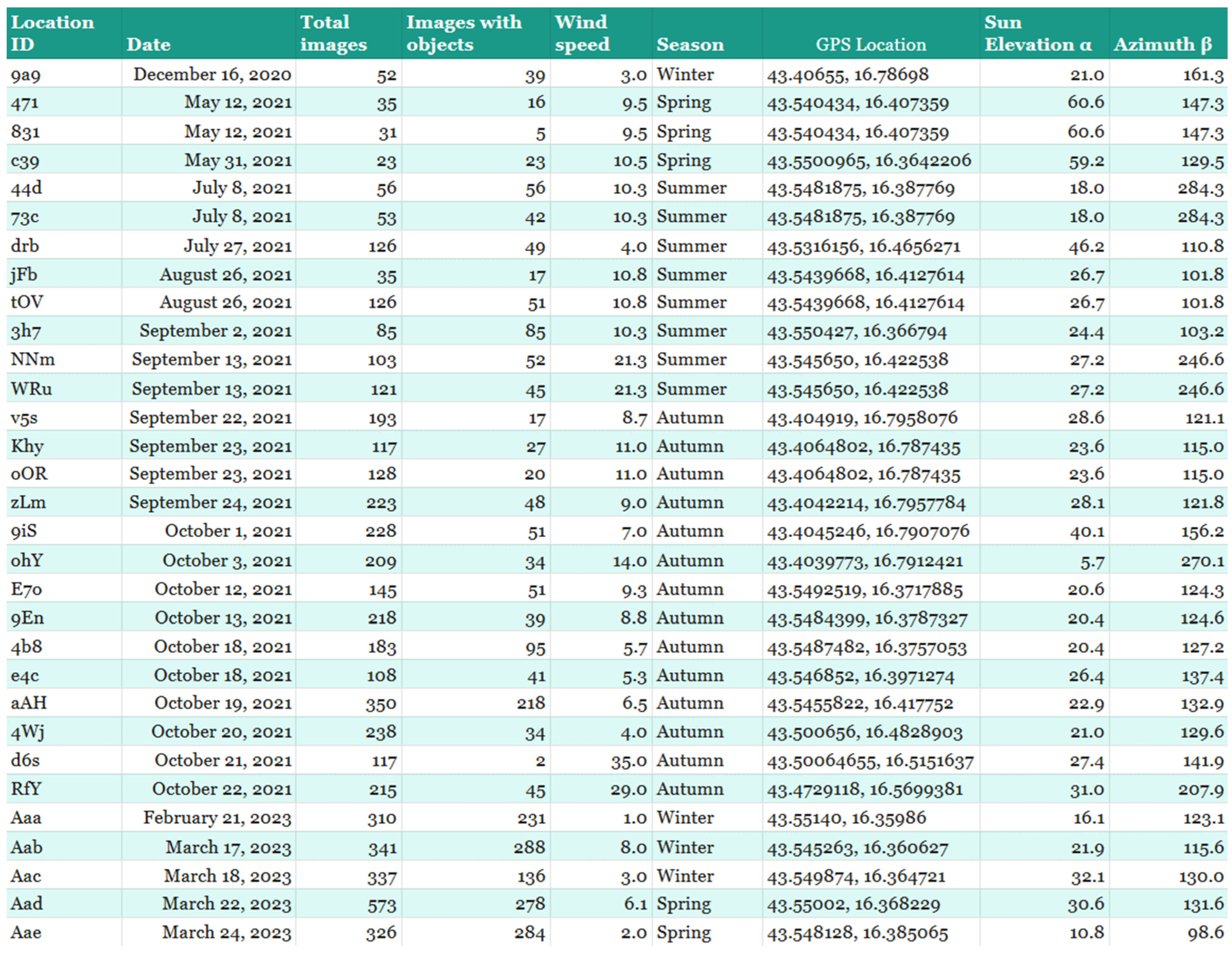
3.1. Database

Before collecting photographs for the database, the following guidelines were set:

• method of data collection has to be remote sensing using UAV
• images should be taken in multiple altitudes—5 m, 10 m, 15 m
• subject of photography—marine debris (litter)
• classes—various non-degradable objects
• photography area—shallow benthic zone (photic zone) with visible litter
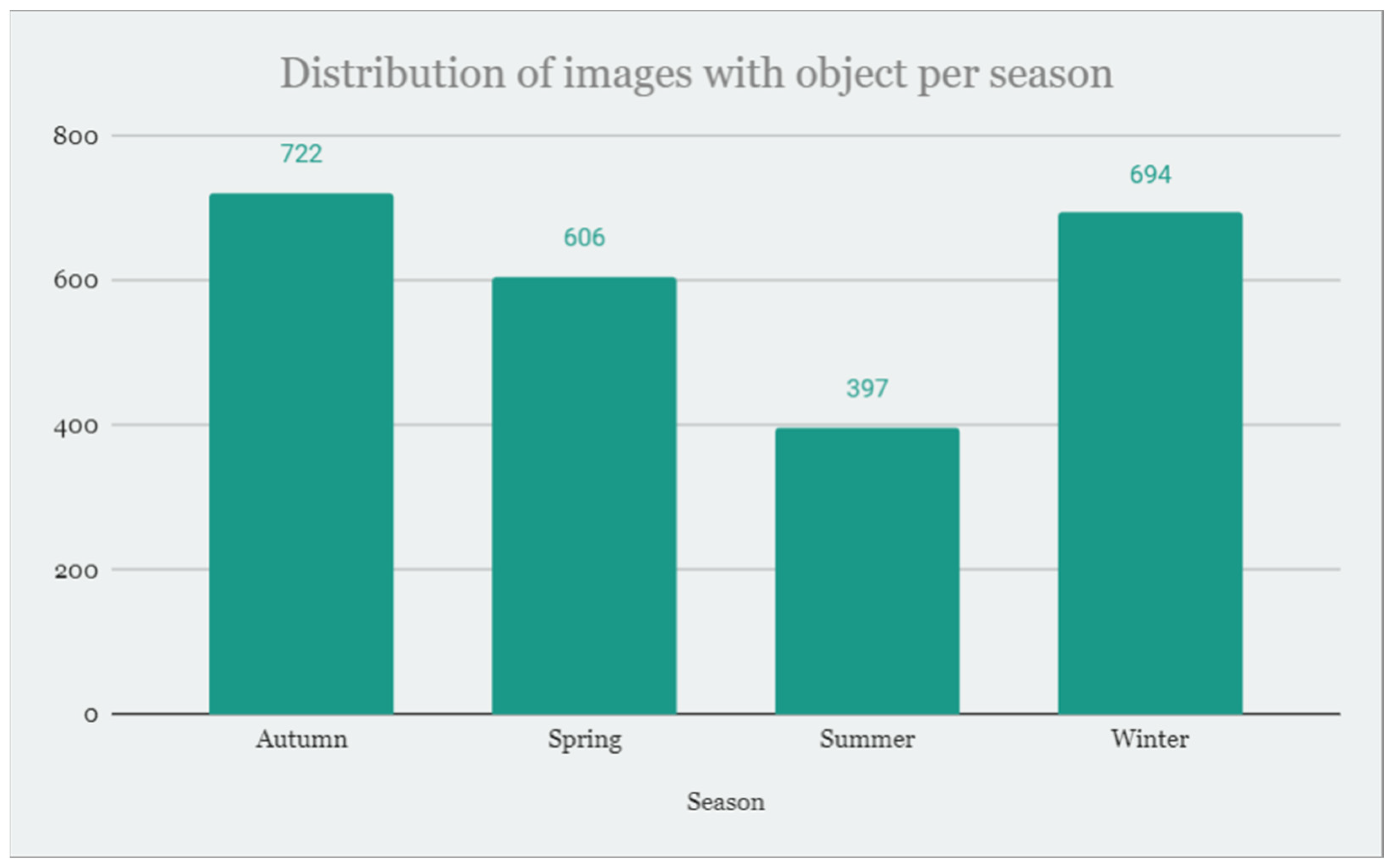
• annual range—during the entire year, seasonal
• time of day—from 6:00 to 20:00 (for various times of daylight)
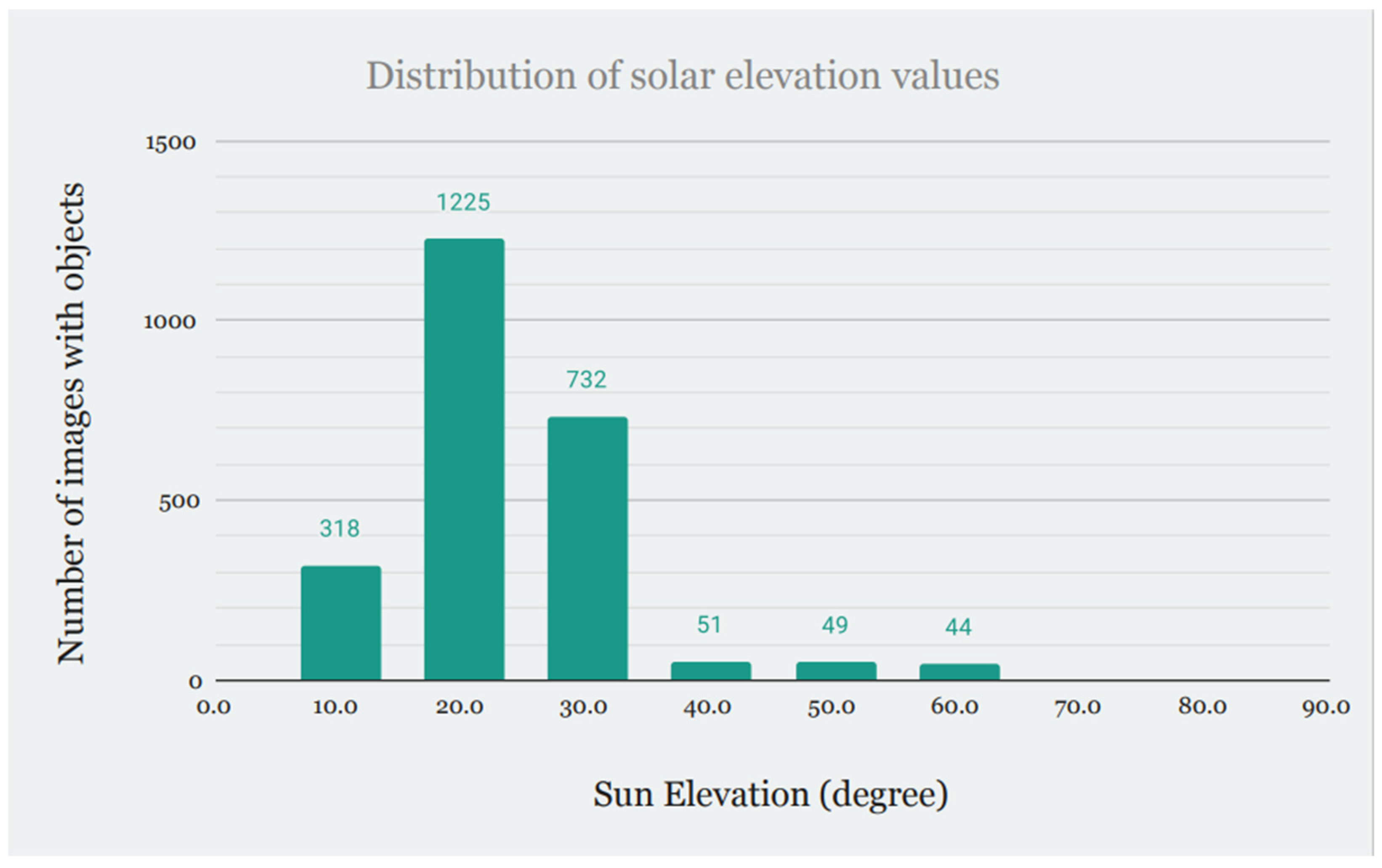
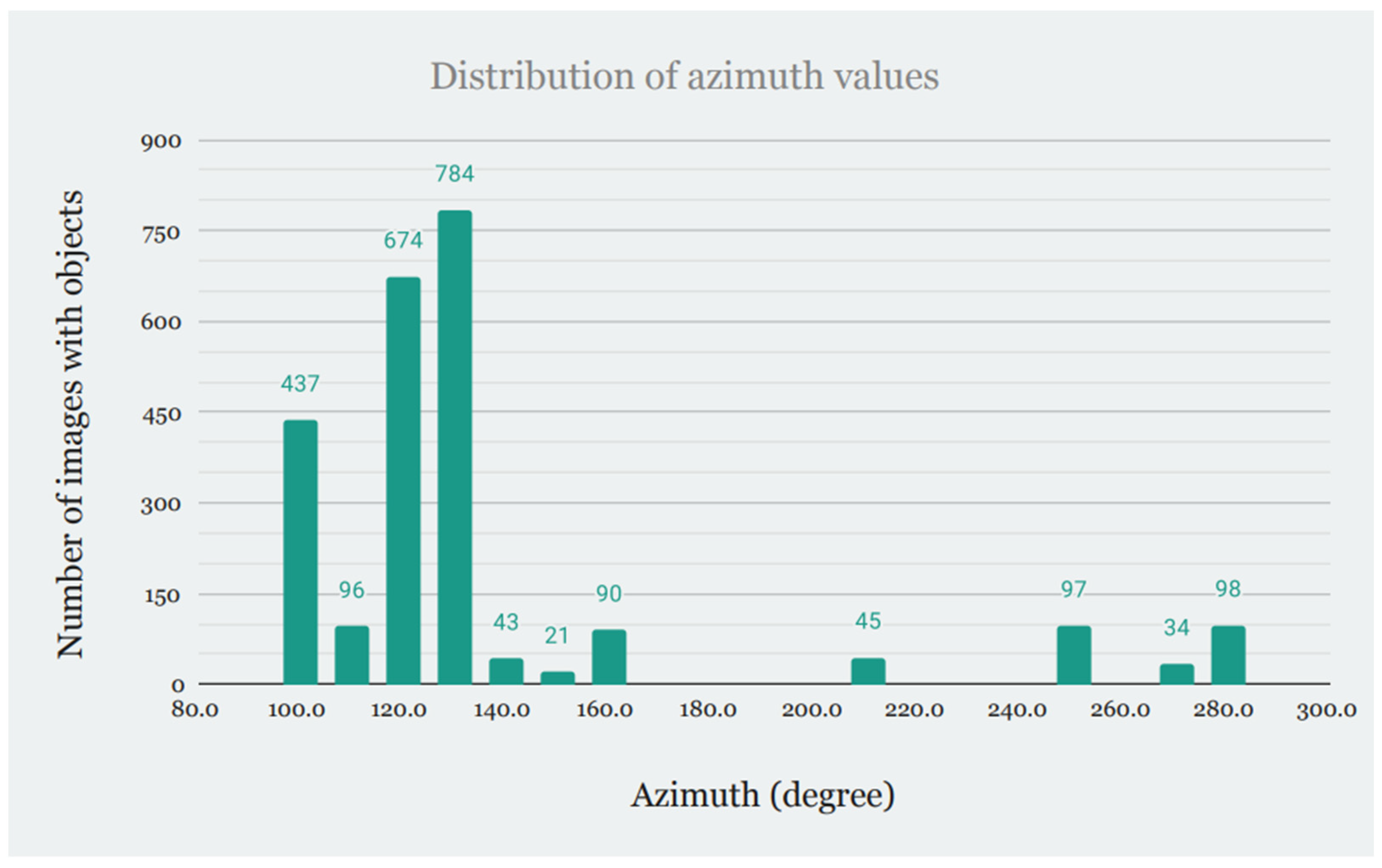
• parameters that should be recorded—date and time, season, GPS coordinates, wind speed and direction, sun elevation, and azimuth

To create a database following the rules that are set above, UAVs DJI Mavic pro 2 camera Hasselblad 20MP 4K UHD and DJI air 2S camera 2.4 µm 5.4K UHD (manufactured by DJI, Shenzen, China) were used to collect images from 5 m, 10 m, and 15 m height.

The photos were taken in the coastal area of the Adriatic Sea in Split-Dalmatia County. Twenty-three locations (stations) are located in the coastal area of the following cities: Kaštela, Vranjic, Split, Stobreč, Podstrana, and Lokva Rogoznica, as shown in Table 1, Figure 1 and zoomed in Figure 2.

Table 1. Location by city and GPS coordinates.

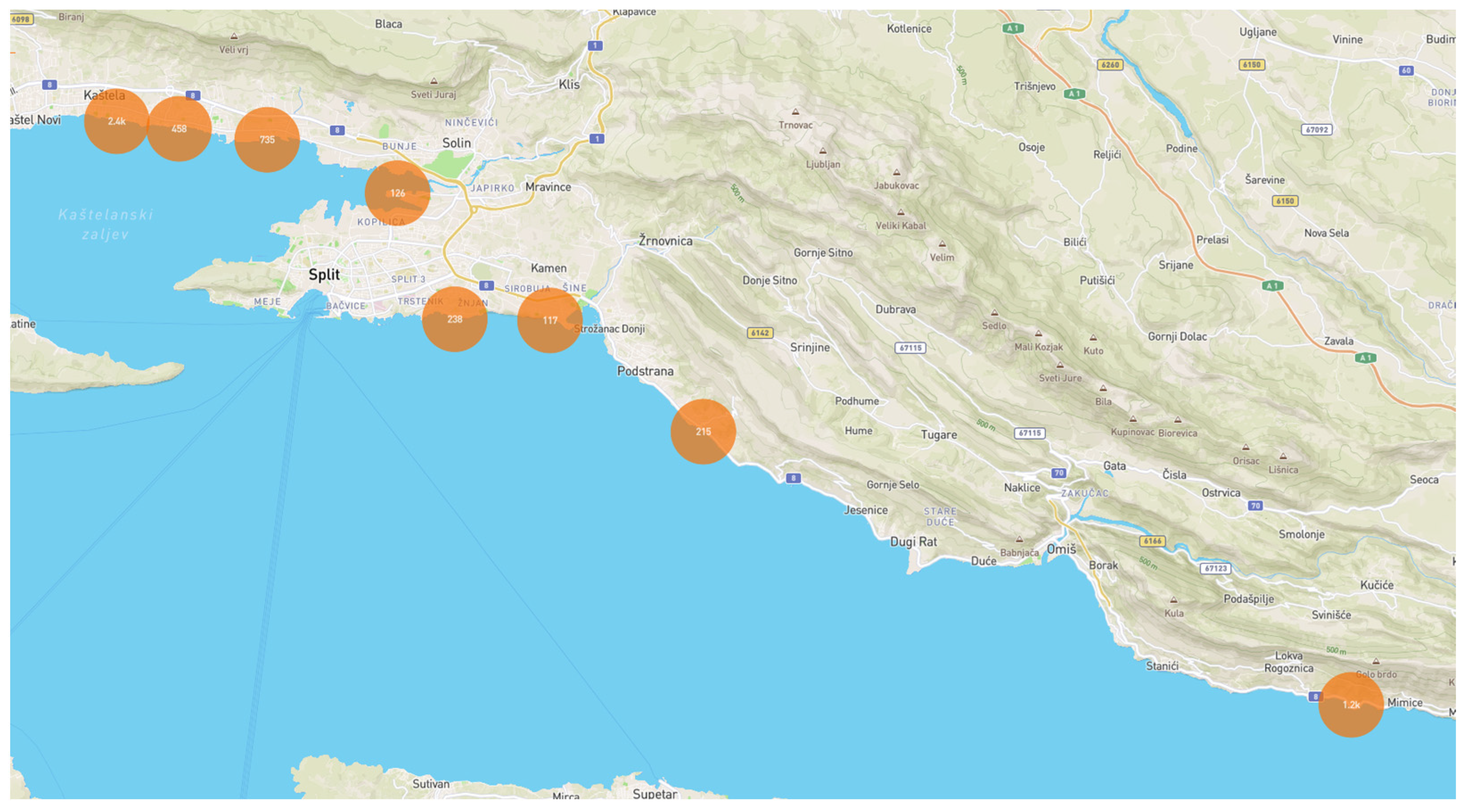
Location	GPS Location
Kaštel Lukšić, Croatia	43.550427, 16.366794
Kaštel Kambelovac, Croatia	43.548128, 16.385065
Kaštel Gomilica, Croatia	43.546852, 16.397127
Kaštel Sućurac, Croatia	43.543966, 16.412761
Vranjic, Croatia	43.531615, 16.465627
beach Žnjan, Split, Croatia	43.500656, 16.482890
Stobreč, Croatia	43.500646, 16.515163
Podstrana, Croatia	43.472911, 16.569938
Lokva Rogoznica, Croatia	43.406480, 16.787435

Figure 1. Locations of all images that are in the dataset (coastal region of Croatia).

Figure 2. The zoomed-in location where each dot represents the location where the image was taken.

Data collection was conducted through all four seasons from December 2021 until March 2023. During the winter, three trips to the field were made, five trips were made during the spring, eight during the summer, and fourteen during the fall, so image distribution was kept similar per season, as shown in Figure 3.

Figure 3. Distribution of images with objects per season.

As shown in Figure 4, the earliest time for photography was at 7:10, and the latest was at 18:30, while the wind speed ranged from 0 km/h to 35 km/h. The number of images present in a specified bucket (by time of the day or by wind speed) is shown in Figure 4 and Figure 5.

Figure 4. Distribution of images per time of day.

Figure 5. Distribution of images by wind speed.

Another key factor in building this kind of database is the position of the sun. As shown in Figure 6 and Figure 7, solar elevation and azimuth were measured to be included in the database (those values are averaged per station instead of per image).

Figure 6. Distribution of solar elevation values.

Figure 7. Distribution of azimuth (an angle between north and projected sun location).

Processing RAW images demands significant computational resources. Therefore, all images were downscaled by a factor of two in both horizontal and vertical resolution and subsequently converted to PNG format. This modified dataset is referred to as the Half Size database. Also, most deep neural networks require smaller images than those in RAW or half-size databases. Resizing again was not a feasible option since the images contained small objects, and resizing would reduce these objects to a few pixels. Therefore, a patch database was created from the halved one, as shown in Figure 8. This database is referred to as the All Patches database. Parts of the images showing the objects were cut out into patches, i.e., a part of the image where labeled objects are located. The patches have dimensions of 640 × 640 pixels and contain one or more objects that are fully or partially visible. This database has 6298 images that are smaller and easier to work with. Since the classes are imbalanced, 9 classes were selected to train with, covering most of the litter found on the seafloor, as shown. These classes were extracted from the All Patches database (summary data presented in Figure 8 and class distribution presented in Figure 9) to create a final Selected Patches database used for preprocessing and training the models. The selected Patches database, shown in Figure 10, consists of 4016 images of 640 × 640 pixels containing the classes: Fragments, Construction material, Tires, Cans, Bottles, Cloth, Bags, Caps and lids, and Cups as shown in Figure 11.

Figure 8. Flowchart of the database creation process.

Figure 9. Distribution of the number of labels per patch in the All Patches database.

Figure 10. Labeled image samples from the All Patches database.

Figure 11. Distribution of classes in the Selected Patches database.

3.2. Preprocessing Methods

Nine preprocessing methods that can improve image quality were selected. CLAHE, ICM, ULAP, GC, MIP, DCP, RGHS, and GBdehazingRCorrection methods collectively address a wide range of issues encountered in underwater photography, including contrast, color distortion, haze, and noise. Each of these methods has been shown to be effective in improving the quality of underwater images, offering reliable results. These methods are adaptable to various underwater conditions, ensuring consistent performance across different scenarios. Therefore, one can ensure a comprehensive and effective approach to preprocessing underwater images, leading to significantly improved image quality [24,25,26,27]. Because underwater environments often suffer from poor visibility due to scattering and absorption of light, which leads to hazy images with low contrast and color distortion, we also chose RoWS, a method that aims to mitigate these issues [28]. Although, in the literature, the mentioned methods are related to the improvement of images taken under the sea surface, it is assumed that their application could also improve aerial images of the seafloor collected by an unmanned aerial vehicle. Each method was implemented per the paper description. Some methods can yield better results if applied after another preprocessing method, so additionally, two methods were combined to test the composability of the preprocessing methods. The proposed database features underwater objects, and while the photographic acquisition process differs, these methods could be effectively utilized.

3.2.1. RoWS (Removal of Water Scattering)

ROWS [28] is a method proposed by Liu Chao and Meng Wang to restore the clarity of underwater images using the dark channel prior. This technique addresses the common issue of underwater images being affected by scattering and attenuation due to particles in the water, which is similar to the effect of heavy fog in the air. The dark channel prior assumes that in most patches of a water-free image, some pixels have very low intensities in at least one color channel. This assumption helps estimate the depth of turbid water and remove its effects, revealing the original clarity of the images. The method involves estimating the background light and transmission map, which are then used to recover the scene radiance. The results show significant improvement in image clarity, making objects appear as if taken in a crystal-clear medium. However, the method does not address the problem of absorption, which affects color restoration. The authors suggest that future work could involve using a fast, soft matting algorithm to improve the transmission map and address the absorption issue. The paper concludes that while the dark channel prior is effective, it may not work well in extreme cases where the scene object is similar to the background light over a large region.

3.2.2. ICM (Integrated Color Model)

ICM [29] is a methodology used to enhance underwater images. The approach involves two main steps: Contrast Stretching of RGB Algorithm and Saturation and Intensity Stretching of HSI (Hue, Saturation, Intensity). The first step is used to equalize the color contrast in the images by stretching the range of the color values to make use of all possible values. Each pixel is scaled using a linear scaling function to maintain the correct color ratio. The second step is used to increase the true color and solve the problem of lighting in underwater images. The HSI model provides a wider color range by controlling the color elements of the image, which helps in enhancing the true color and brightness of the images. The contrast stretching algorithm enhances image contrast by expanding the range of color values to utilize the entire spectrum of possible values. This process employs a linear scaling function to adjust the pixel values [30]. Each pixel is scaled according to this function, as shown in Equation (1):

$$P_o=\left(P_i-c\right)\times {\displaystyle \frac{\left(b-c\right)}{\left(d-c\right)}}+a$$

(1)

where P_o is the normalized pixel value, P_i is the considered pixel value, a is the minimum value of the desired range, b is the maximum value of the desired range, c is the lowest pixel value currently present in the image, d is the highest pixel value currently present in the image.

3.2.3. CLAHE (Contrast-Limited Adaptive Histogram Equalization)

CLAHE [31] is a technique used in image processing to improve the contrast of images. Unlike traditional histogram equalization, which applies the same transformation to all pixels in an image, CLAHE operates on small regions in the image called tiles. Each tile’s histogram is equalized, and the neighboring tiles are then combined using bilinear interpolation to eliminate artificially induced boundaries. CLAHE is a modified version of the AHE technique [32]. While AHE can cause excessive noise amplification in underwater images, CLAHE mitigates this issue by dividing the image into several sub-blocks and performing histogram equalization on each part individually. However, CLAHE has its drawbacks, including the generation of ring and noise artifacts in the flat regions of images. The new pixel value J is calculated using the following Equation (2):

$$J=\left(j_{max}-j_{min}\right)\times P\left(f\right)+j_{min}$$

(2)

where j is the new value of the pixel, and P(f) is the cumulative probability distribution of pixel values in an image. This distribution is used for various image processing techniques, including CLAHE, to enhance the contrast of an image. Specifically, P(f) represents the cumulative distribution function (CDF) of the pixel intensities in the image, which is used to transform the pixel values to improve the overall contrast and visibility of details in the image [24].

3.2.4. ULAP (Underwater Light Attenuation Prior)

ULAP [33] is a concept used in underwater image restoration to estimate scene depth. The principle behind ULAP is that the scene depth increases with the higher value of the difference between the maximum value of green (G) and blue (B) lights (simplified MVGB) and the value of red (R) light (simplified as VR) in an underwater image. This difference is used to train a linear model for scene depth estimation, which is crucial for restoring underwater images by estimating background light and transmission maps. Based on the ULAP, a linear model of the MVGB and VR for the depth map estimation is developed as follows, as shown in Equation (3):

$$d\left(x\right)={\mu }_0+{\mu }_{1}m\left(x\right)+{\mu }_{2}v\left(x\right)$$

(3)

where x represents a pixel, d(x) is the underwater scene depth at point x, m(x) is the MVGB, v(x) is the VR.

3.2.5. GC (Gamma Correction Model)

GC [34] is a technique used to adjust the brightness of an image to improve its visual quality. It changes the relationship between the input and output brightness of an image, resulting in a more natural appearance. This means that darker parts of the image can be brightened, and brighter parts can be darkened to achieve a balanced display. Applying gamma correction can significantly enhance the contrast of an image, making details more visible. This is particularly useful in situations where images are too dark or too bright. In specific applications such as underwater photography, gamma correction can help restore natural colors that are lost due to light absorption in water. It is simple to implement and does not require complex calculations, making it practical for various real-time applications.

3.2.6. MIP (Maximum Intensity Prior)

MIP [35] is a concept used in image deblurring. The MIP algorithm was originally proposed for the display of MRA imaging, where the interest is to show vessels over the background of tissues in an image. It is based on the observation that the maximum value of local patch pixels and gradients decreases during the blurring process. The MIP is a combination of two priors: the local maximum intensity (LMI) and the local maximum gradient (LMG). By combining these two priors, the MIP enhances the latent image, which is beneficial for the estimation of the blur kernel and improves the quality of the deblurred image. The MIP is used in a new energy function for image deblurring, which is optimized using an alternating optimization strategy. This approach has been shown to be more effective compared to state-of-the-art methods in various experiments.

3.2.7. DCP (Dark Channel Prior)

DCP [36] is a technique used in image processing, specifically for image dehazing. It is based on the observation that in most natural haze-free images, some pixels (in a local patch) have very low intensity in at least one color channel. This observation is used to estimate the thickness of the haze and subsequently remove it from the image. The DCP method operates under the assumption that the transmission is locally constant, which can lead to halo artifacts at depth discontinuities. As shown in Equation (4), the Dark Channel Prior asserts that the local minimum of the darkest color channel in a haze-free image of a natural scene tends to be zero.

$$J^{\mathrm{dark}}\left(x\right)=\underset{y\in \mathsf{\Omega }\left(x\right)}{\min }\left(\underset{c\in \{r,g,b\}}{\min }{J}^c\left(y\right)\right)\to 0$$

(4)

where $J^c\left(\mathrm{y}\right)$ is intensity of the color channel c at pixel y, $\mathsf{\Omega }\left(x\right)$ is a local patch centered at x, $\underset{y\in \mathsf{\Omega }}{\mathrm{m}\mathrm{i}\mathrm{n}}$ finds the minimum value within the local patch, $\underset{c\in \{r,g,b\}}{\mathrm{m}\mathrm{i}\mathrm{n}}$ finds the minimum intensity among the red, green and blue channels at pixel y. To improve the dehazing results, various methods have been proposed to refine the transmission estimation, such as using guided filters (GF).

3.2.8. RGHS (Relative Global Histogram Stretching)

RGHS [37] is a method proposed for enhancing shallow-water images, which often suffer from low contrast, fuzziness, and color cast due to light absorption and scattering underwater. In the RGB color space, RGHS first equalizes the green (G) and blue (B) channels. It then redistributes each R-G-B channel histogram using dynamic parameters that relate to the intensity distribution of the original image and the wavelength attenuation of different colors underwater. Bilateral filtering is used to eliminate noise while preserving valuable details and enhancing local information of the image. Color Correction is performed by stretching the L component and modifying the a and b components in the CIE-Lab color space. This step aims to improve the saturation and brightness of the image to obtain more vivid colors. RGHS can achieve better perceptual quality, higher image information entropy, and less noise compared to state-of-the-art underwater image enhancement methods. It effectively balances the chroma, saturation, and contrast of the enhanced underwater images.

3.2.9. GBdehazingRCorrection (Single Underwater Image Restoration by Blue-Green Channels Dehazing and Red Channel Correction)

GBdehazingRCorrection [38] is a method for enhancing the quality of underwater images, which are often degraded due to light absorption and scattering in water. The method involves two main steps: Blue-Green Channels Dehazing and Red Channel Correction. The blue and green channels of the underwater image are processed using a dehazing algorithm. This algorithm is based on an extension and modification of the DCP algorithm, which is commonly used for dehazing terrestrial images. The DCP algorithm helps in estimating the medium transmission map and background light, which are then used to recover the blue and green channels of the image, as shown in Equation (5):

$$t\left(x\right)=1-\underset{c\in \{g,b\}}{\min }\left(\underset{x\in \mathsf{\Omega }}{\min }\left({\displaystyle \frac{I^c\left(x\right)}{B^c}}\right)\right)$$

(5)

where $t\left(x\right)\in \left[\mathrm{0,1}\right]$ is the medium transmission map which represents the percentage of the scene radiance reaching the camera, $I^c\left(x\right)$ is the observed intensity of the pixel x in the channel c, where c can be either green g or blue b, $B^c$ is the background light intensity for the channel c, $\underset{c\in \{g,b\}}{\mathrm{m}\mathrm{i}\mathrm{n}}$ selects the minimum value among the green and blue channels, $\underset{x\in \mathsf{\Omega }}{\mathrm{m}\mathrm{i}\mathrm{n}}$ computes the minimum ratio of the observed intensity to the background light within the local patch.

The haze-free channel can be restored by Equation (6):

$$J^c\left(x\right)={\displaystyle \frac{I^c\left(x\right)-B^c}{t^c\left(x\right)}}+B^c,\hspace{1em}c\in \{g,b\}$$

(6)

where $J^c\left(x\right)$ represents the restored channel.

The red channel, which suffers more from absorption in water, is corrected using the Gray-World assumption theory. This theory assumes that the average color of an image should be gray. By adjusting the red channel based on this assumption, the method compensates for the color distortion and enhances the visibility of the red channel, as shown in Equation (7).

$${\displaystyle \frac{avgRr+avgBr+avgGr}{3}}=0.5$$

(7)

where avgRr, avgBr and avgGr are the normalized average values of the recovered red, blue, and green channel, respectively.

The average value of the recovered red channel can be estimated as follows:

$$avgRr=1.5-avgBr-avgGr$$

(8)

the compensation coefficient δ can be calculated as:

$$\delta ={\displaystyle \frac{avgRr}{avgR}}$$

(9)

where avgR is the normalized average value of the original red channel.

The recovered red channel Rrec can be obtained by the following equation:

$$Rrec=R\times \delta$$

(10)

where R is the normalized original red channel, and δ is the estimated compensation coefficient.

Additionally, the method includes an adaptive exposure map to address the issue of some regions in the recovered image appearing too dim or too bright. This map helps in adjusting the exposure of different regions of the image to achieve better visual quality. The proposed method significantly improves the visibility, contrast, and color balance of underwater images, outperforming existing methods in both qualitative and quantitative evaluations.

3.3. Neural Networks for Detection and Classification

Image preprocessing methods were used to create 13 datasets on which models are going to be trained. Some of the methods used to preprocess images are a combination of other two methods, applying one method after another to aquire the final image. Those models have two underscores in the name denoting which methods were used and in which order. Separate models were built for each of the preprocessed datasets and trained using the transfer learning method. The YOLOv8 architecture was employed, with the OpenImageV7 68.7M (YOLOv8x-oiv7) model serving as the base, which was further refined through transfer learning. Two other models were trained: one that contains original patches (without any preprocessing) and one that does not include a transfer learning method. The training was conducted within 100 epochs with patience set to 30, using the AdamW optimizer, a learning rate of 0.000769, and a momentum of 0.937 [39]. Numbers are recommended by YOLOv8 researchers (based on empirical testing and existing research). The dataset was divided into three splits: training, testing, and validation, with a commonly chosen 60/20/20 ratio (2394/809/813 images) [40]. In total, fifteen different models were trained, one for each prepared dataset and two with unmodified datasets. Models None and None no transfer are used as a baseline to compare other results. RoWS, ICM, CLAHE, and ULAP were selected because previous research has suggested positive and improved results. Those preprocessing methods were used exclusively. Combinations (like CLAHE__GC and others) were chosen by concluding what each method does and combining them on each photograph to possibly achieve better results.

4. Results

This section verifies that the use of appropriate database and preprocessing methods will improve the quality of images with underwater objects and thus improve the accuracy and precision of the algorithm for detecting underwater objects.

4.1. New Database

Given that a database of underwater objects photographed by UAVs does not exist or is not public, our own database was built, and the following link provides information about the database https://codeasy.com/seafloor-litter-database (accessed on 28 August 2024).

The database consists of 5405 original images. Of those 5405 images, there are 2419 images, 44.8% of which have underwater litter present, while the rest, 55.2%, do not. In addition to the date of photography, location, GPS coordinates, wind speed, type of wind, and season, the angle of solar elevation and azimuth were calculated. Each station is assigned a unique prefix and serial image number, as shown in Figure 12.

Figure 12. Stations metadata.

The database consists of 12,786 objects classified into 31 classes: Fragments, Constructional material, Tires, Cans, Bottles, Ropes, Cloth, Bags, Fishing tools, Caps, and lids, Cups, Buckets, Pipe, Footwear, Cartons, Dishes, Paper, Chain, Chair, Shopping carts, Trash can, Road sign, Dumpster, Boats, Glove, Car parts, Traffic cone, Flipper, Scooter, Electric drill and Cigarette butt as shown in Figure 13.

Figure 13. Distribution of categories.

Many images have multiple different objects present at the same time, so the distribution of objects per image is also shown in Figure 14. It can be seen that most of the images have one or two objects present, but there are images with more than 30 objects present.

Figure 14. Distribution of a number of labels per single image.

Images are in RAW format (DNG), which has been converted to PNG format, and they have been resized to make them smaller (width and height have been halved). PNG images are currently in two resolutions (depending on what UAV was used): 2732 × 1820 and 2732 × 1535. All the images have been hand-labeled and organized, as shown in Figure 15.

Figure 15. Samples from the database.

4.2. Preprocessing Methods Results

4.2.1. Metrics

In target detection, boxes can be classified as true targets or false targets, resulting in four possible outcomes: true positive (TP), false positive (FP), true negative (TN), and false negative (FN). If the Intersection over Union (IoU) between the detected box and the true box exceeds the threshold, the detected box is labeled as TP. Otherwise, it is labeled as FP. If no detected box matches the true box, it is labeled as FN. TP indicates the number of correctly identified targets, FP represents the number of incorrectly identified targets, and FN denotes the number of targets that were not detected. The model’s performance is typically evaluated using precision (Pr) and recall (Re), which are calculated using Equations (11) and (12).

$$Pr={\displaystyle \frac{TP}{FP+TP}}$$

(11)

$$Re={\displaystyle \frac{TP}{FN+TP}}$$

(12)

Precision (Pr) and recall (Re) are interrelated metrics. When precision remains high while recall increases, it indicates that the model is performing better. Conversely, a model with lower performance may experience a significant drop in precision to achieve higher recall. The Precision-Recall curve was used to describe model efficacy. It delineates the relationship between precision (the proportion of true positive predictions among all positive predictions) and recall (the proportion of true positive predictions among all actual positives). The area under the Precision-Recall curve (AUC-PR) serves as an indicator of a model’s capability to sustain precision across different recall thresholds. In this paper, the threshold of the intersection over union (IOU) between the prediction bounding box and the target bounding box is selected to be greater than 0.5 as the criterion for judging target detection. All results are calculated for detections where confidence is more than 0.45, and IoU is more than 0.5. Those values are chosen for historical reasons (PASCAL VOC Challenge uses this value) and comparability (because it is widely adapted, it allows researchers to compare their results against others in a consistent manner).

4.2.2. Results

The model “None no transfer” refers to the model trained on a dataset without any preprocessing and without using the transfer learning method. The model “None” indicates that no preprocessing was applied, but transfer learning was used. The results of the analysis of different models for image processing, precision, recall, and F1-Score are presented in Table 2.

Table 2. Preprocessing method inference results.

Model	Precision	Recall	F1-Score
RoWS	81.22%	44.80%	57.74%
None	77.42%	44.94%	56.87%
ICM	73.78%	44.99%	55.89%
CLAHE	77.89%	43.33%	55.68%
RoWS__ULAP	75.04%	42.10%	53.94%
CLAHE__GC	73.60%	42.34%	53.75%
CLAHE__ICM	66.15%	40.21%	50.01%
CLAHE__MIP	66.15%	40.21%	50.01%
ULAP	72.69%	37.65%	49.61%
DCP__MIP	75.99%	35.34%	48.24%
GC__ICM	65.81%	37.42%	47.71%
GC__RGHS	65.81%	37.42%	47.71%
None no transfer	65.06%	31.88%	42.79%
GBdehazingRCorrection__RoWS	76.56%	29.66%	42.75%
GBdehazingRCorrection__UDCP	76.56%	29.66%	42.75%

The RoWS model achieved the highest F1-Score of 57.74%, while the model None no transfer had the lowest F1-Score of 42.79%. Models like CLAHE and ICM showed solid performance with F1-Scores of 55.68% and 55.89%, respectively. Models such as GC__ICM and GC__RGHS had comparable results with an F1-Score of 47.71%. These data highlight the variability in the performance of different models in image processing, emphasizing the importance of selecting the appropriate approach for specific needs.

As shown in the confusion matrix in Figure 16, the highest values are concentrated along the diagonal of the matrix, indicating that the model has correctly classified instances for each category, which suggests an effective model. The confusion matrix indicates that the model performs very well in identifying fragments. However, there are instances where Fragments or Construction materials were not identified at all (visible in the (none) column). The concentration of positive values along the diagonal and zero values off-diagonal suggests that the model performs well but has issues with missing detections.

Figure 16. Confusion matrix for RoWS model at IoU@0.5.

Figure 17 plots the Precision-Recall curve with IoU@0.5 and shows a single number summary of the PR-Curve (representing the area under the curve, AP). Tires exhibit the highest average precision, indicating that models can distinguish tires from other categories effectively. Fragments and Cans show moderate performance. Bags, Bottles, and other categories show lower AP. This can be attributed to the amorphous and semi-transparent structure, which makes it difficult for models to extract object shapes and features.

Figure 17. Precision-Recall curve for RoWS model at IoU@0.5.

As shown in Table 3, results reveal significant variability in the performance of object recognition using the RoWS method across different object classes. The precision, recall, and F1-score metrics indicate that the method is particularly effective for recognizing tires, which achieved high precision (87%), recall (70%), and F1-score (78%). Conversely, the method struggled with cups, which had the lowest metrics, with precision at 67%, recall at 14%, and an F1-score of 24%, which we can attribute to a database not containing enough images with different variations of cups. Other objects, such as fragments, cans, and bottles, showed moderate performance, with precision ranging from 75% to 84% and recall between 43% and 54%, resulting in F1 scores around 54% to 64%. Construction materials exhibited a high precision of 90% but a low recall of 25%, indicating that while the method is accurate when it detects these materials, it misses many instances. Overall, the RoWS method demonstrates varied effectiveness, excelling in categories like tires while showing limitations in others like cups and cloth.

Table 3. Performance metrics of object recognition using RoWS methods across different object classes.

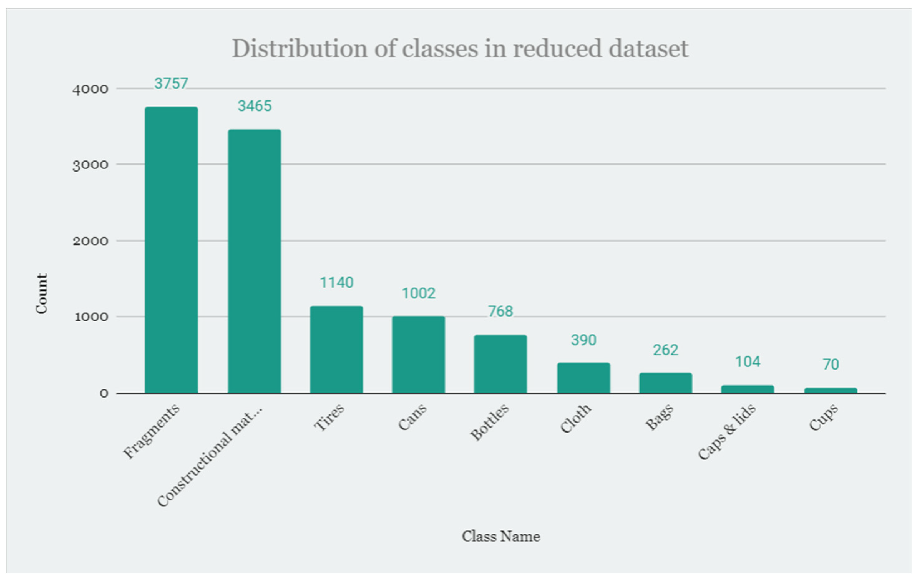
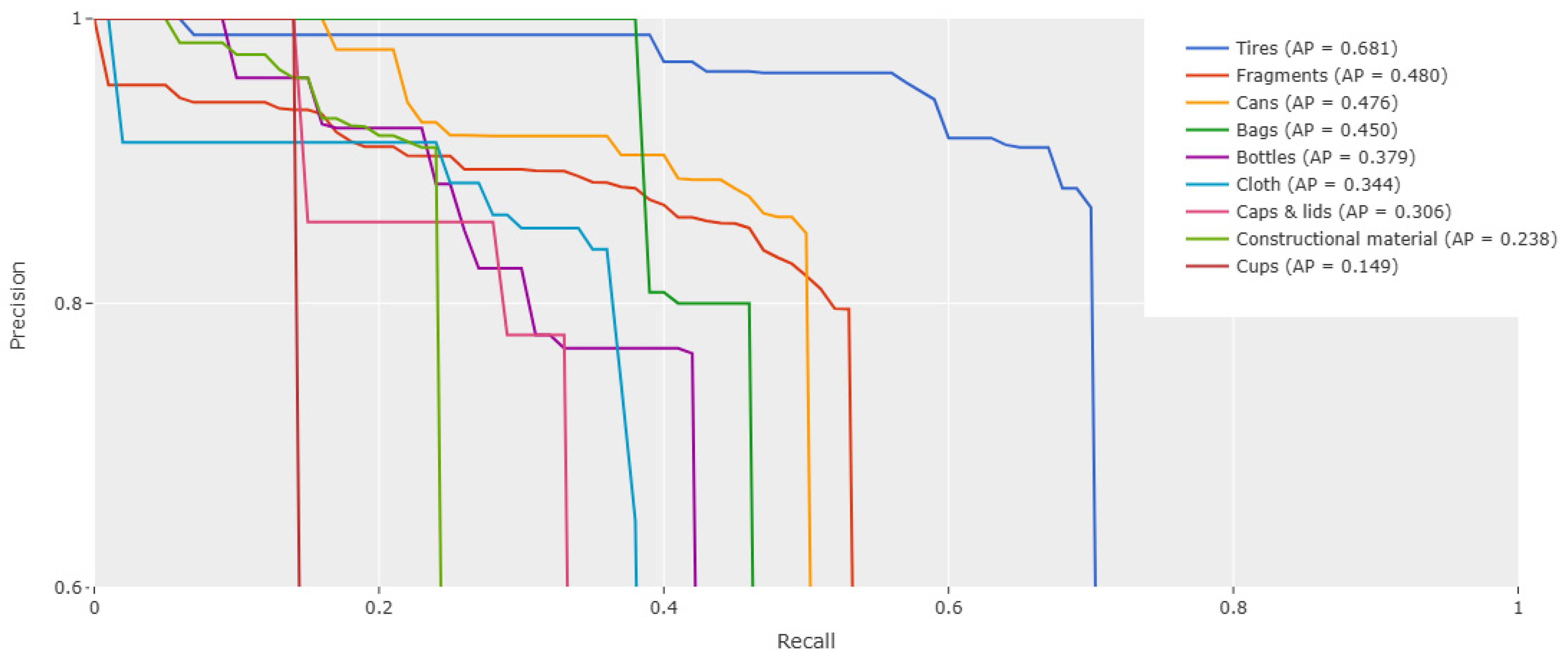
Class	Objects	Precision	Recall	F1-Score
Fragments	3757	79%	54%	64%
Constructional material	3465	90%	25%	39%
Tires	1140	87%	70%	78%
Cans	1002	84%	50%	63%
Bottles	768	75%	43%	54%
Cloth	390	65%	39%	49%
Bags	262	80%	46%	59%
Caps and lids	104	78%	33%	47%
Cups	74	67%	14%	24%

5. Conclusions

This research presents a comprehensive approach to detecting marine debris using UAVs through advanced image preprocessing and deep learning techniques. A significant contribution of this study is the development of a novel database with over 5000 images and more than 12,000 objects categorized into 31 classes. The database is enriched with metadata such as GPS location, wind speed, sun elevation, and azimuth, which enhances the context and usability of the data. The study introduces various image preprocessing methods to improve the detection of underwater objects, with the RoWS method showing the best performance. The YOLOv8 architecture with the OpenImageV7 68.7 M (YOLOv8x-oiv7) model serving as the base for the transfer learning was implemented for the detection and classification of seafloor objects. The proposed approach improves detection precision compared to the original results without pre-processing of the input images. Future work should focus on getting images from various locations and creating a larger database. Of course, adding sea depth information to the metadata of images in the database could be interesting for researchers, although these values are not immutable because they depend on the tidal cycle. Also, it takes quite a bit of time to determine the precise depth value in each image (location). Furthermore, some of the research should focus on novel techniques to remove waves and optical distortion of the images by augmenting the existing neural network with special ones. Overall, the findings demonstrate that the appropriate use of databases and preprocessing methods can enhance the accuracy and precision of underwater object detection algorithms, offering a promising solution to the challenge of marine litter detection and environmental monitoring.

References

- Simonyan, K.; Zisserman, A. Very Deep Convolutional Networks for Large-Scale Image Recognition. arXiv 2015, arXiv:1409.1556. Available online: http://arxiv.org/abs/1409.1556 (accessed on 15 June 2022).
- Darby, J.; Clairbaux, M.; Bennison, A.; Quinn, J.L.; Jessopp, M.J. Underwater visibility constrains the foraging behaviour of a diving pelagic seabird. Proc. R. Soc. B Biol. Sci. 2022, 289, 20220862. [Google Scholar] [CrossRef] [PubMed]
- Liu, Y.; Xu, H.; Zhang, B.; Sun, K.; Yang, J.; Li, B.; Li, C.; Quan, X. Model-Based Underwater Image Simulation and Learning-Based Underwater Image Enhancement Method. Information 2022, 13, 187. [Google Scholar] [CrossRef]
- Kislik, C.; Genzoli, L.; Lyons, A.; Kelly, M. Application of UAV Imagery to Detect and Quantify Submerged Filamentous Algae and Rooted Macrophytes in a Non-Wadeable River. Remote Sens. 2020, 12, 3332. [Google Scholar] [CrossRef]
- Politikos, D.V.; Fakiris, E.; Davvetas, A.; Klampanos, I.A.; Papatheodorou, G. Automatic detection of seafloor marine litter using towed camera images and deep learning. Mar. Pollut. Bull. 2021, 164, 111974. [Google Scholar] [CrossRef]
- Marin, I.; Mladenović, S.; Gotovac, S.; Zaharija, G. Deep-Feature-Based Approach to Marine Debris Classification. Appl. Sci. 2021, 11, 5644. [Google Scholar] [CrossRef]
- Ships in Satellite Imagery. Available online: https://www.kaggle.com/rhammell/ships-in-satellite-imagery (accessed on 31 March 2022).
- Yabin, L.; Jun, Y.; Zhiyi, H. Improved Faster R-CNN Algorithm for Sea Object Detection Under Complex Sea Conditions. Int. J. Adv. Netw. Monit. Control. 2020, 5, 76–82. [Google Scholar] [CrossRef]
- Lorencin, I.; Anđelić, N.; Mrzljak, V.; Car, Z. Marine Objects Recognition Using Convolutional Neural Networks. Naše More 2019, 66, 112–120. [Google Scholar] [CrossRef]
- Lin, W.-H.; Zhong, J.-X.; Liu, S.; Li, T.; Li, G. ROIMIX: Proposal-Fusion Among Multiple Images for Underwater Object Detection. In Proceedings of the ICASSP 2020—2020 IEEE International Conference on Acoustics, Speech and Signal Processing (ICASSP), Barcelona, Spain, 4–8 May 2020; pp. 2588–2592. [Google Scholar] [CrossRef]
- Li, J.; Skinner, K.A.; Eustice, R.M.; Johnson-Roberson, M. WaterGAN: Unsupervised Generative Network to Enable Real-time Color Correction of Monocular Underwater Images. IEEE Robot. Autom. Lett. 2017, 3, 387–394. [Google Scholar] [CrossRef]
- Hong, J.; Fulton, M.S.; Sattar, J. TrashCan 1.0 An Instance-Segmentation Labeled Dataset of Trash Observations. 23 July 2020. Available online: https://conservancy.umn.edu/items/6dd6a960-c44a-4510-a679-efb8c82ebfb7 (accessed on 7 May 2022).
- Sasaki, T.; Azuma, S.; Matsuda, S.; Nagayama, A.; Ogido, M.; Saito, H.; Hanafusa, Y. JAMSTEC E-library of Deep-Sea Images (J-EDI) Realizes a Virtual Journey to the Earth’s Unexplored Deep Ocean. Abstract #IN53C-1911. 2016. Available online: https://ui.adsabs.harvard.edu/abs/2016AGUFMIN53C1911S/abstract (accessed on 1 August 2022).
- Hong, J.; Fulton, M.; Sattar, J. TrashCan: A Semantically-Segmented Dataset towards Visual Detection of Marine Debris. arXiv 2020, arXiv:2007.08097. Available online: http://arxiv.org/abs/2007.08097 (accessed on 29 October 2021).
- Hong, J.; Fulton, M.; Sattar, J. A Generative Approach towards Improved Robotic Detection of Marine Litter. In Proceedings of the 2020 IEEE International Conference on Robotics and Automation (ICRA), Paris, France, 31 May–31 August 2020; pp. 10525–10531. [Google Scholar] [CrossRef]
- Krizhevsky, A.; Sutskever, I.; Hinton, G.E. ImageNet Classification with Deep Convolutional Neural Networks. In Proceedings of the Advances in Neural Information Processing Systems, Lake Tahoe, NV, USA, 3–6 December 2012; Curran Associates, Inc.: New York, NY, USA, 2012. Available online: https://proceedings.neurips.cc/paper/2012/hash/c399862d3b9d6b76c8436e924a68c45b-Abstract.html (accessed on 15 June 2022).
- Fabbri, C.; Islam, M.J.; Sattar, J. Enhancing Underwater Imagery Using Generative Adversarial Networks. In Proceedings of the 2018 IEEE International Conference on Robotics and Automation (ICRA), Brisbane, QLD, Australia, 21–25 May 2018; pp. 7159–7165. [Google Scholar] [CrossRef]
- ImageNet. Available online: https://www.image-net.org/index.php (accessed on 31 March 2022).
- Martin, C.; Zhang, Q.; Zhai, D.; Zhang, X.; Duarte, C.M. Drone images of sandy beaches and anthropogenic litter along the Saudi Arabian Red Sea. Mendeley Data 2021, 1. [Google Scholar] [CrossRef]
- Martin, C.; Zhang, Q.; Zhai, D.; Zhang, X.; Duarte, C.M. Anthropogenic litter density and composition data acquired flying commercial drones on sandy beaches along the Saudi Arabian Red Sea. Data Brief 2021, 36, 107056. [Google Scholar] [CrossRef] [PubMed]
- Garcia-Garin, O.; Monleón-Getino, T.; López-Brosa, P.; Borrell, A.; Aguilar, A.; Borja-Robalino, R.; Cardona, L.; Vighi, M. Automatic detection and quantification of floating marine macro-litter in aerial images: Introducing a novel deep learning approach connected to a web application in R. Environ. Pollut. 2021, 273, 116490. [Google Scholar] [CrossRef] [PubMed]
- The EUVP Dataset|Interactive Robotics and Vision Lab. Available online: http://irvlab.cs.umn.edu/resources/euvp-dataset (accessed on 11 March 2022).
- Naseer, A.; Baro, E.N.; Khan, S.D.; Vila, Y. A Novel Detection Refinement Technique for Accurate Identification of Nephrops norvegicus Burrows in Underwater Imagery. Sensors 2022, 22, 4441. [Google Scholar] [CrossRef]
- Alsakar, Y.M.; Sakr, N.A.; El-Sappagh, S.; Abuhmed, T.; Elmogy, M. Underwater Image Restoration and Enhancement: A Comprehensive Review of Recent Trends, Challenges, and Applications. Preprints 2023, 2023070585. [Google Scholar] [CrossRef]
- Song, W.; Liu, Y.; Huang, D.; Zhang, B.; Shen, Z.; Xu, H. From shallow sea to deep sea: Research progress in underwater image restoration. Front. Mar. Sci. 2023, 10, 1163831. [Google Scholar] [CrossRef]
- Yang, M.; Hu, J.; Li, C.; Rohde, G.; Du, Y.; Hu, K. An In-Depth Survey of Underwater Image Enhancement and Restoration. IEEE Access 2019, 7, 123638–123657. [Google Scholar] [CrossRef]
- Wang, Y.; Song, W.; Fortino, G.; Qi, L.-Z.; Zhang, W.; Liotta, A. An Experimental-Based Review of Image Enhancement and Image Restoration Methods for Underwater Imaging. IEEE Access 2019, 7, 140233–140251. [Google Scholar] [CrossRef]
- Liu, C.; Meng, W. Removal of water scattering. In Proceedings of the 2010 2nd International Conference on Computer Engineering and Technology, Chengdu, China, 16–18 April 2010; pp. V2-35–V2-39. [Google Scholar] [CrossRef]
- Point Operations—Contrast Stretching. Available online: https://homepages.inf.ed.ac.uk/rbf/HIPR2/stretch.htm (accessed on 28 June 2024).
- Iqbal, K.; Salam, R.A.; Osman, A.; Talib, A.Z. Underwater Image Enhancement Using an Integrated Colour Model. IAENG Int. J. Comput. Sci. 2007, 34, IJCS_34_2_1. [Google Scholar]
- Pizer, S.M.; Johnston, R.E.; Ericksen, J.P.; Yankaskas, B.C.; Muller, K.E. Contrast-limited adaptive histogram equalization: Speed and effectiveness. In Proceedings of the [1990] Proceedings of the First Conference on Visualization in Biomedical Computing, Atlanta, GA, USA, 22–25 May 1990; pp. 337–345. [Google Scholar] [CrossRef]
- Mustafa, W.; Kader, M. A Review of Histogram Equalization Techniques in Image Enhancement Application. J. Phys. Conf. Ser. 2018, 1019, 012026. [Google Scholar] [CrossRef]
- Song, W.; Wang, Y.; Huang, D.; Tjondronegoro, D. A Rapid Scene Depth Estimation Model Based on Underwater Light Attenuation Prior for Underwater Image Restoration. In Advances in Multimedia Information Processing—PCM 2018; Hong, R., Cheng, W.-H., Yamasaki, T., Wang, M., Ngo, C.-W., Eds.; Lecture Notes in Computer Science; Springer International Publishing: Cham, Switzerland, 2018; Volume 11164, pp. 678–688. ISBN 978-3-030-00775-1. [Google Scholar] [CrossRef]
- Xiang, W.; Yang, P.; Wang, S.; Xu, B.; Liu, H. China Underwater image enhancement based on red channel weighted compensation and gamma correction model. Opto-Electron. Adv. 2018, 1, 18002401–18002409. [Google Scholar] [CrossRef]
- Hu, D.; Tan, J.; Zhang, L.; Ge, X.; Liu, J. Image deblurring via enhanced local maximum intensity prior. Signal Process. Image Commun. 2021, 96, 116311. [Google Scholar] [CrossRef]
- Song, Y.; Luo, H.; Hui, B.; Chang, Z. An improved image dehazing and enhancing method using dark channel prior. In Proceedings of the 27th Chinese Control and Decision Conference (2015 CCDC), Qingdao, China, 23–25 May 2015; pp. 5840–5845. [Google Scholar] [CrossRef]
- Huang, D.; Wang, Y.; Song, W.; Sequeira, J.; Mavromatis, S. Shallow-Water Image Enhancement Using Relative Global Histogram Stretching Based on Adaptive Parameter Acquisition. In MultiMedia Modeling; Schoeffmann, K., Chalidabhongse, T.H., Ngo, C.W., Aramvith, S., O’Connor, N.E., Ho, Y.-S., Gabbouj, M., Elgammal, A., Eds.; Lecture Notes in Computer Science; Springer International Publishing: Cham, Switzerland, 2018; Volume 10704, pp. 453–465. ISBN 978-3-319-73602-0. [Google Scholar] [CrossRef]
- Li, C.; Quo, J.; Pang, Y.; Chen, S.; Wang, J. Single underwater image restoration by blue-green channels dehazing and red channel correction. In Proceedings of the 2016 IEEE International Conference on Acoustics, Speech and Signal Processing (ICASSP), Shanghai, China, 20–25 March 2016; pp. 1731–1735. [Google Scholar] [CrossRef]
- ultralytics/ultralytics/cfg/default.yaml at main ultralytics/ultralytics. GitHub. Available online: https://github.com/ultralytics/ultralytics/blob/main/ultralytics/cfg/default.yaml (accessed on 22 August 2024).
- Training, Validation, Test Split for Machine Learning Datasets. Available online: https://encord.com/blog/train-val-test-split/ (accessed on 22 August 2024).