A Green Wave Ecological Global Speed Planning under the Framework of Vehicle–Road–Cloud Integration

Abstract

In response to energy consumption and traffic efficiency reduction caused by intersection congestion, a global speed planning that considered both ecological speed and green wave speed was conducted under the vehicle–road–cloud integration framework. After establishing an instantaneous energy consumption model for pure electric vehicles, a radial basis neural network model was used to estimate the queue length of traffic flow, and an isolated-intersection-based eco-approach and departure (I-EAD) plan was proposed based on a valid traffic signal light model. A two-stage optimization multi-intersections-based eco-approach and departure (M-EAD) strategy with multiple objectives and constraints was proposed to solve the optimal green light window and the optimal speed trajectory. The results of the SUMO/Matlab/Simulink/Python joint simulation platform show that the M-EAD strategy reduces the average travel energy consumption by 16.65% and 8.31%, and the average travel time by 26.33% and 12.53%, respectively, compared to the intelligent driver model (IDM) and I-EAD strategy. The simulation results of the typical traffic scenarios and random traffic scenarios indicate that the speed optimization strategies in this study have good optimization effects on energy conservation and traffic efficiency.

1. Introduction

Due to the control effect of traffic signals, vehicles may experience frequent starting, stopping, and idling during the process of passing through signalized intersections. Signal intersections, as key points in urban road networks, are high-risk areas for vehicle congestion and environmental pollution. At present, with the rapid increase in household vehicle ownership, traditional traffic signal control technology is no longer sufficient to solve transportation problems such as traffic congestion, safety issues, energy waste, and environmental pollution. Reasonable speed planning can increase the probability of vehicles passing through signalized intersections without stopping. It can improve traffic efficiency and reduce unnecessary energy consumption and emissions, which is an important way to achieve the goals of carbon neutrality and carbon emissions peak. Related studies have shown that reasonable speed planning at signalized intersections can improve overall traffic efficiency by 6–18% [1].

Transportation optimization has been given more possibilities with the booming development of the intelligent connected vehicle industry [2] and vehicle–road collaboration technology [3]. Internet of Vehicles (IoV) technology collects and recognizes environmental and status information on vehicles through devices such as GPS, RFID, sensors, and cameras [4]. Communication between the onboard unit (OBU) and roadside unit (RSU), including vehicle-to-vehicle (V2V), vehicle-to-infrastructure (V2I), vehicle-to-pedestrian (V2P), and vehicle-to-network (V2N) is achieved through communication methods such as 5G, LTE, PC5, etc. [5,6]. With the help of Internet technology, perceived information can be gathered and transmitted to the central processor and then be analyzed and processed through cloud computing technology to provide a variety of services, including optimal route and speed planning, traffic signal arrangement, real-time road condition reporting, etc. [7]. Green wave speed guidance, as a new type of intelligent transportation application function, utilizes vehicle road coordination technology to achieve real-time data interaction between connected vehicles and roadside units, obtain accurate intersection signal status, and combine current vehicle position, speed, and other status information to break away from the limitations of traditional fixed green wave speed belt.

At the same time, with the continuous development of vehicle–road–cloud integration technology [8], green wave speed guidance has gradually evolved from a technology solution based on vehicle-road interaction to a technology solution based on vehicle–road–cloud architecture. The vehicle–road–cloud integration-based speed guidance can simultaneously optimize the speed of multiple signal intersections and multiple road sections under the unified monitoring of the control center while avoiding the time delay caused by dedicated short-range communication between the vehicles and roadside units [9]. The powerful computing and multi-source information fusion capabilities of the cloud can greatly accelerate the computing speed, ensure the real-time provision of green wave speed, and enable connected vehicles to pass through continuous signal intersections, which can improve traffic efficiency and reduce energy consumption.

2. Related Works

In terms of improving traffic efficiency, researchers have mainly used two methods to enable vehicles to pass through intersections without stopping: the first one is adjusting the signal phase. Adaptive signal control technology (ASCT) is a traffic management strategy that adjusts signal timing parameters to optimize corridor performance based on actual traffic demand [10]. Shams, A. et al. [11] compared quantitatively the performance of 11 methods of offset optimization, including several different objectives that make use of arrival profiles (e.g., maximizing arrivals on the green, minimizing delay, minimizing the number of stops) and several different methods of bandwidth maximization. The second is to adjust the vehicle’s operating speed, which is also the direction of improvement in this study.

2.1. Green Wave Speed Planning

Scholars have conducted extensive research on green wave speed induction strategies for urban signalized intersections. These strategies can be mainly divided into two types based on different decision control methods: the rule-based speed induction control method and the optimization-based speed induction control method [12].

The rule-based speed induction control method is simple with small computational complexity and fast calculation speed. HomChaudhuri, B. et al. [13,14] used a uniform speed model to solve the velocity of vehicles passing through intersections. Ala, M.V. et al. [15,16] used a uniform acceleration model to solve the optimal vehicle speed for vehicles passing through intersections. Barth, M.J. et al. [17,18] proposed a trigonometric function model to calculate the target average speed of vehicles by analyzing the timing of traffic signals and the distance between the vehicle and the stop line at the intersection. Based on this, they guided the vehicle to perform acceleration and deceleration operations to ensure passing through the intersection without stopping. Kari, D. et al. [19] developed a green wave speed control algorithm that considered parameters such as the current speed, position, signal cycle, phase, and offsets. They divided the situation of vehicles passing through intersections into acceleration, deceleration, and stopping scenarios, and determined whether the vehicle can pass through the intersection at a constant speed during the current or adjacent green light time based on current speed. The rule-based speed guidance control method has poor control accuracy and optimization effect, which is mainly suitable for simple control scenarios at isolated signal intersections.

The optimization-based speed induction control method is based on multi-objective and multi-constrained optimization models to obtain the optimal vehicle speed trajectory. Wu, W. et al. [20] proposed a comprehensive traffic control model that optimized both vehicle speed and traffic signals. They developed speed guidance strategies targeting vehicle arrival time, delay, and stopping numbers at red and green light conditions, respectively. Some scholars considered vehicle dynamic characteristics and energy consumption as constraints for green wave speed planning. The optimization-based speed induction control method is widely used in speed planning for continuous signalized intersections. Compared to speed planning for isolated signalized intersections, speed planning for continuous signalized intersections produces better energy-saving effects [21].

In recent years, with the booming development of the intelligent connected vehicle industry and vehicle-road collaboration technology, many scholars have introduced connected vehicle scenarios into speed optimization. Wang, Q.Z. et al. [22] proposed a decentralized approach to the optimization CAV trajectories in both longitudinal and lateral dimensions along a signalized arterial under the mixed traffic environment, where human vehicles (HVs) and CAVs co-exist. Talukder, M.A.S. et al. [23] developed an approach to use vehicle trajectory data with traditional traffic signal controllers, even with the lower penetration rate of CV-enabled vehicles on the road and the limited deployment of vehicle-to-infrastructure (V2I) communications. Several scholars have proposed collaborative optimization control methods of intersection signal control and vehicle speed guidance under the vehicle–road–cloud integration framework to improve the efficiency of the mainline traffic and verify the methods through simulation. The position and speed of arriving vehicles were used to calculate their estimated time of arrival [24]. Dong, H. et al. [25] proposed a green wave speed induction strategy for connected vehicles considering the queuing phenomenon at signalized intersections. They assumed that the queue length at intersections was known and combined it with a vehicle dynamics model to predict the dissipation time of traffic queues. Zhang, C. et al. [26] proposed a vehicle speed planning method based on real-time estimation of queue length for connected vehicles on multiple signalized intersections in dynamic traffic environments. Simulation results showed that this method could generate smoother vehicle speed curves and reduce energy consumption by more than 40% compared with traditional speed planning methods, ignoring traffic queues. The use of V2X wireless communication technology can achieve wide area information sharing and resource integration, leading speed induction based on vehicle–road–cloud integration to a new research direction.

2.2. Ecological Speed Planning

Eco-driving is the optimal energy consumption and efficient driving trajectory under the constraints of the driving environment and vehicle power system [27]. The goal of eco-approach and departure (EAD) is optimizing vehicle speed to avoid stop-and-go behavior at signalized intersections, which can be mainly divided into two strategies: isolated-intersection-based eco-approach and departure (I-EAD) and multi-intersections-based eco-approach and departure (M-EAD).

Some researchers have tended to focus on vehicle dynamics and kinematics. Bautista-Montesano, R. et al. [28] proposed rule- and fuzzy-inference system-based strategies for a coupled eco-approach and departure regenerative braking system through a numerical simulator and a three-degree-of-freedom connected electric vehicle model. The simulations aimed to compare both longitudinal navigation strategies utilizing relevant metrics: power, efficiency, comfort, and usage duty cycle in motor and generator modes. Other researchers tended to focus on speed planning. Jin, H. et al. [29] calculated the instantaneous fuel consumption of vehicles at different speeds and used these speed sequences as weights for the spatiotemporal topology of traffic signals. Simulation results showed that it could improve fuel economy by 33.6% and reduce travel time by 17.7%. Based on the vehicle’s status and the signal phase information of traffic lights, the traffic characteristics of the vehicle were judged, and the ecological speed trajectory with the minimum average fuel consumption was solved using a fuel consumption model by Meng, Z. et al. [30]. The simulation results showed that using this model could reduce fuel consumption by at least 10%. Most existing EAD studies envision an ideal setting that neglects real-world operational conditions such as lane changes, multi-movement intersection configuration, partially automated fleet, and/or limited traffic state awareness [31]. Dong, H.X. et al. [32] proposed an overtaking-enabled eco-approach control (OEAC) strategy to potentially mitigate the negative effect on the movement of the following vehicle by the preceding vehicle. Most studies are based on simulation verification, but there are also a few studies based on real vehicle verification. Vehicle-level testing of the optimized speed profiles was carried out at the American Center of Mobility (ACM) on GM-Volt Gen II to demonstrate an energy-saving of 40–50 kJ per intersection on real road conditions [33].

There is no doubt that a typical application scenario of ecological driving is under the framework of vehicle–road–cloud integration. The connected vehicles use V2X communication to interact with roadside units or the cloud through communication 4G, 5G, DSRC, etc., to obtain information such as signal phase and timing (SPaT), speed limits, and stopping line positions. Adjusting the vehicle speed promptly and smoothly at the green light phase thereby can reduce frequent acceleration and deceleration behavior, energy loss, and travel time delays. Yang, J.S. et al. [34] proposed a less-disturbed ecological driving strategy for connected and automated vehicles combining offline planning and online tracking. In offline planning, an energy-efficient reference speed is created based on traffic information (such as the average traffic speed) and characteristics of the vehicle (such as the engine efficiency map) via dynamic programming. In online tracking, model predictive control is employed to update the vehicle speed in real-time to track the reference speed. Some researchers have considered the combination of green wave speed and ecological speed. Han, J.H. et al. [35] found that a longitudinal fuel-optimal speed trajectory could be a control sequence of four possible modes: maximum acceleration, constant speed cruising, coasting, and maximum braking. They presented a fast analytical solver that computes the longitudinal fuel-optimal speed trajectory for connected and automated vehicles. Virginia Tech Transportation Institute (VTTI) [36] conducted a study on speed planning for isolated signal intersections based on a V2I environment. The vehicle’s current speed and the passable time of the intersection were used to determine the acceleration, deceleration, and uniform driving states that the vehicle should adopt. Then, the VT-Micro (Virginia Tech microscopic) model was used to calculate the fuel consumption of different driving states, and the lowest fuel consumption solution was provided to the driver through a human-computer interaction interface.

In summary, although scholars have conducted extensive research in the field of speed guidance, there is still room for improvement: (1) Under the vehicle–road–cloud integration framework, numerous V2I facilities can perceive more comprehensive environmental information. The powerful storage and computing capabilities of cloud computing make it possible to optimize global speed based on historical data. The range of speed guidance has expanded from short road sections or isolated intersections to continuous multiple signalized intersections, and factors such as the impact of social vehicle queues should also be considered. (2) How to achieve the organic integration of green wave speed and ecological speed goals, taking into account both traffic efficiency and energy consumption, is an urgent technical problem that needs to be solved (3) The existing research on ecological green wave speed planning mostly focuses on fuel vehicles. As entering the era of electrification, research on speed induction strategies based on the energy consumption characteristics of pure electric vehicles should be strengthened.

3. Methodology

3.1. Assumptions

Due to the mutual influence between green wave speed planning and signal phase coordination, to clarify and highlight the research object, the control object of this study was set as a single connected vehicle under the framework of vehicle–road–cloud integration without considering the fleet situation. The following assumptions were proposed:

• The study only focused on controlling the speed of connected vehicles, and the signal phases were already in an optimal state. To simplify the calculation, the signal phase and time cycle at the same intersection were fixed and unchanged;
• The study only considered the queue length of other social vehicles as influencing factors, without taking into account the operation influences of other non-connected vehicles and non-motorized vehicles in the road sections during driving;
• The study only considered that vehicles pass through the multiple intersections directly, without considering lane changing and overtaking behaviors;
• Communication delays were ignored when transmitting information between connected vehicles, roadside units, and cloud control platforms, and there were no information losses.

3.2. Energy Consumption Model

3.2.1. Instantaneous Energy Consumption Model

When an EV travels at a speed of v ($\mathrm{m}/\mathrm{s}$) and an acceleration of a $(\mathrm{m}/{\mathrm{s}}^2)$, the driving resistance of the vehicle is acceleration resistance $F_a$, rolling resistance $F_r$, air resistance $F_k$, and slope resistance $F_g$, respectively. Therefore, the driving force $F_t$ exerted on the vehicle traveling at speed v and acceleration a can be represented by the total vehicle mass m (kg), the slope angle θ (°) of the road, the conversion factor of rotating mass δ, the rolling resistance constant µ, and the air resistance constant k, that is:

$$F_t=F_a+F_r+F_k+F_g$$

(1)

$$F_a=\delta ma$$

(2)

$$F_r=mg\mu$$

(3)

$$F_k=k{v}^2$$

(4)

$$F_g=mg\sin \theta$$

(5)

An instantaneous energy consumption model for pure electric connected vehicles was constructed based on the principle of power balance. The energy consumption power of the vehicle, which is the input power P of the motor, consists of two parts: the output power p and the power loss $P_{copper}$.

$$P=p+P_{copper}$$

(6)

The first part is the traction power generated for driving the vehicle, which is related to the current vehicle speed and the instantaneous traction force. Therefore, the output power p of a vehicle with a speed of v can be established based on the driving force $F_t$:

$$p=F_t·v$$

(7)

The second part is the power loss $P_{copper}$ generated by the motor’s heat loss, which is mainly caused by copper heat loss. According to Ohm’s law, copper heat loss can be calculated using the following formula:

$$P_{copper}=I^2·r$$

(8)

where $I$ is the current (A) and r is the impedance (Ω).

In addition, the relationship of a direct-current (DC) generator between the driving force $F_t$, and the current I is as follows:

$$F_t={\displaystyle \frac{K_a\varphi i_0}{R}}·I=KI$$

(9)

where K is defined as the formula $K={\displaystyle \frac{K_a\varphi i_0}{R}}$. $K_a$ is the inherent armature constant of the DC motor; $\varphi$ is the magnetic flux on the armature; R is the rolling radius of the wheel; $i_0$ is the transmission ratio of the transmission system.

Substituting Formula (9) into Formula (6) yields the following formula:

$$P={\displaystyle \frac{r}{K^2}}{F_t}^2+F_t\nu$$

(10)

Substituting Formulas (1)–(5) into Formula (10) yields the following formula:

$$\begin{gathered} P[\nu (t),a(t)]={\displaystyle \frac{r}{K^2}}(\delta ma(t)+k{v}^2(t)+mg\mu +mg\mathit{sin}\theta {)}^2 \\ +\nu (t)(\delta ma(t)+k{\nu }^2(t)+mg\mu +mg\mathit{sin}\theta ) \end{gathered}$$

(11)

Formula (11) is the instantaneous energy consumption model of electric vehicles, which indicates that the input power P is the function of speed v and acceleration a. When the acceleration is less than 0, that is, the vehicle is undergoing a deceleration process, and the energy consumption model can also represent the process of regenerative braking energy recovery.

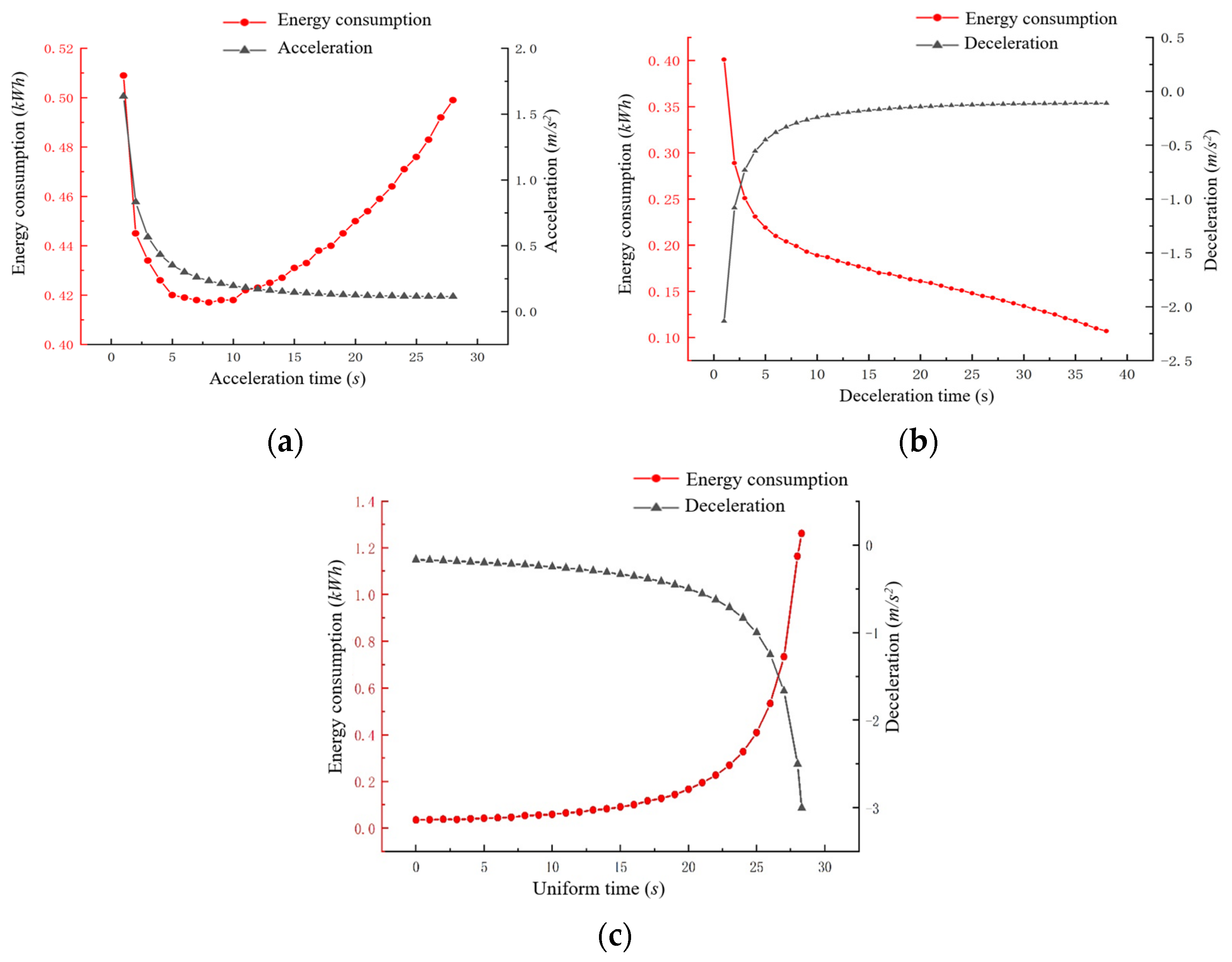
3.2.2. Optimal Energy Consumption Model under Different Scenarios

Traditional vehicles often experience urgent acceleration, deceleration, or stopping at intersections due to the inability to predict traffic lights’ signal phase, resulting in additional energy consumption. For the convenience of research, the driving trajectory of the vehicle was simplified into two stages: uniform acceleration/deceleration driving and uniform driving. The speed optimization trajectory diagram of the optimal energy consumption model was developed for three scenarios: acceleration, deceleration, and stopping.

As shown in Figure 1a for the acceleration scenario, at a distance d (km) from the intersection, the vehicle accelerates uniformly at a certain acceleration rate $a_a$ to the target speed $v_c$, and then maintains a constant speed $v_c$ to pass through the signalized intersection, where the acceleration time is $t_a$ and the constant speed time is $t_c$. Considering energy consumption and comfort issues, vehicles should be guided to arrive at the signalized intersection before the end of the green phase $t_1$. There are two edge situations: when accelerating at the minimum acceleration, the vehicle undergoes a longer uniform acceleration process to the maximized speed while passing through the intersection; when accelerating at the maximum acceleration, the vehicle experiences a shorter uniform acceleration time to the minimized, which satisfies safety and comfort. There are countless speed trajectories between the two edge situations. Different speed trajectories will result in different energy consumption. The optimal energy consumption model aims to find a speed trajectory that minimizes energy consumption under the conditions of time constraints, dynamic constraints, and kinematic constraints. The speed optimization trajectory diagrams under the deceleration and stopping scenarios are similar to the acceleration scenario, as shown in Figure 1b,c. In the deceleration scenario, the vehicle decelerates first and then passes through the intersection at a constant speed. In the stopping scenario, the vehicle first maintains a constant speed and then decelerates to a speed of 0 at the stopping line.

Figure 1. The speed optimization trajectory diagram of different scenarios: (a) acceleration scenario; (b) deceleration scenario; and (c) stopping scenario.

The green wave speed planning process’s total energy consumption power (kWh) is calculated using the instantaneous energy consumption model for electric vehicles in Formula (11). The green wave speed at signalized intersections is optimized to minimize average energy consumption power per unit distance f (kWh/km). The objective function for ecological vehicle speed is:

$$f=\mathit{min}\left({\displaystyle \frac{J}{d}}\right)=min{\displaystyle \frac{\int P\left[a\right(t),v(t\left)\right]d_t}{d}}$$

(12)

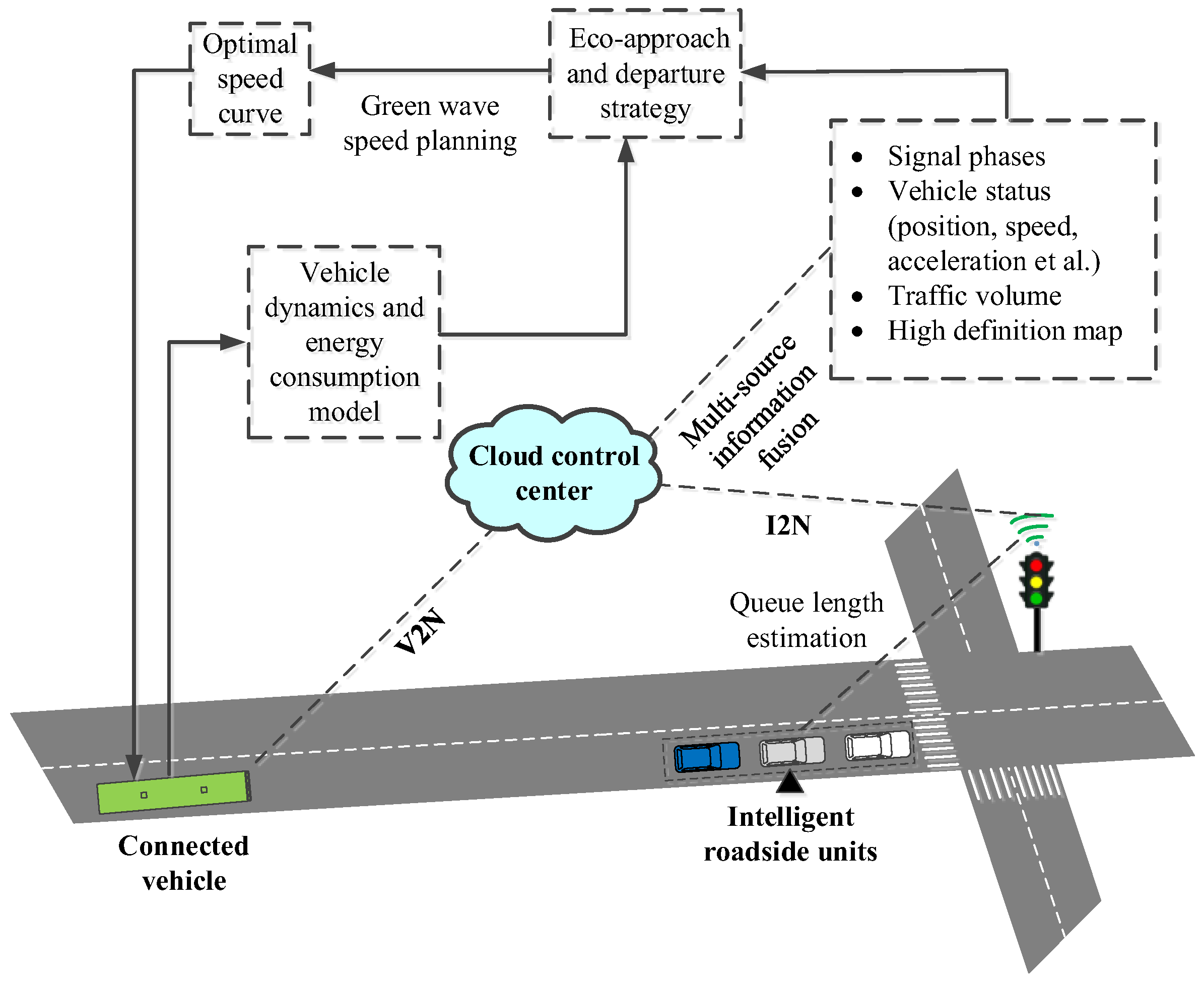
3.3. Isolated-Intersection-Based Eco-Approach and Departure Strategy (I-EAD)

The system framework of I-EAD for an isolated intersection is shown in Figure 2. When the connected vehicles implement the green wave speed induction strategy, the onboard unit and roadside unit obtain information and send the relevant information to the cloud control center through vehicle-to-network (V2N) and infrastructure-to-network technology, respectively. The cloud control center uses powerful multi-source information fusion and computing capabilities to process the information, estimate the queue length, and design optimal speed curves based on energy consumption models for three scenarios. Green wave speed recommendation schemes are provided and sent to the corresponding connected vehicles.

Figure 2. System framework of I-EAD.

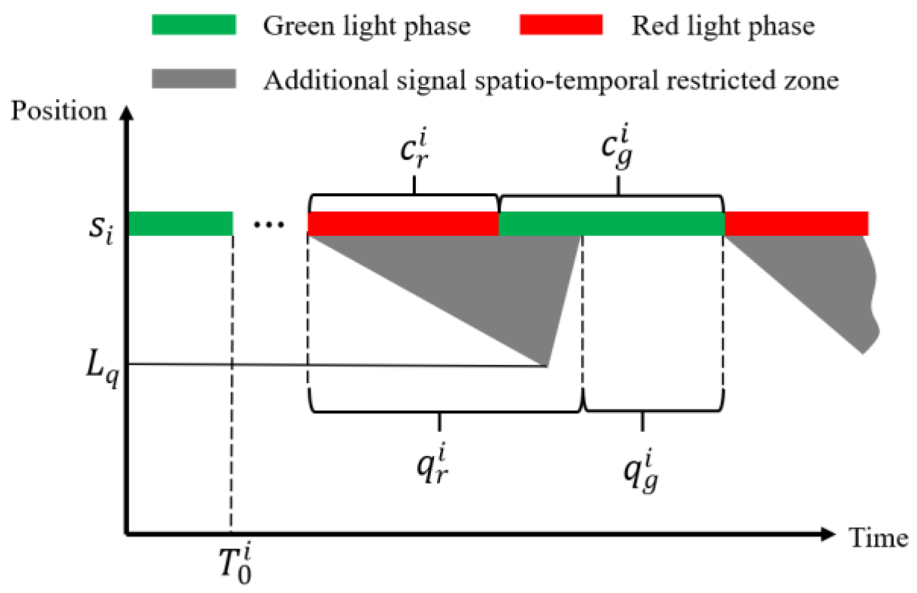
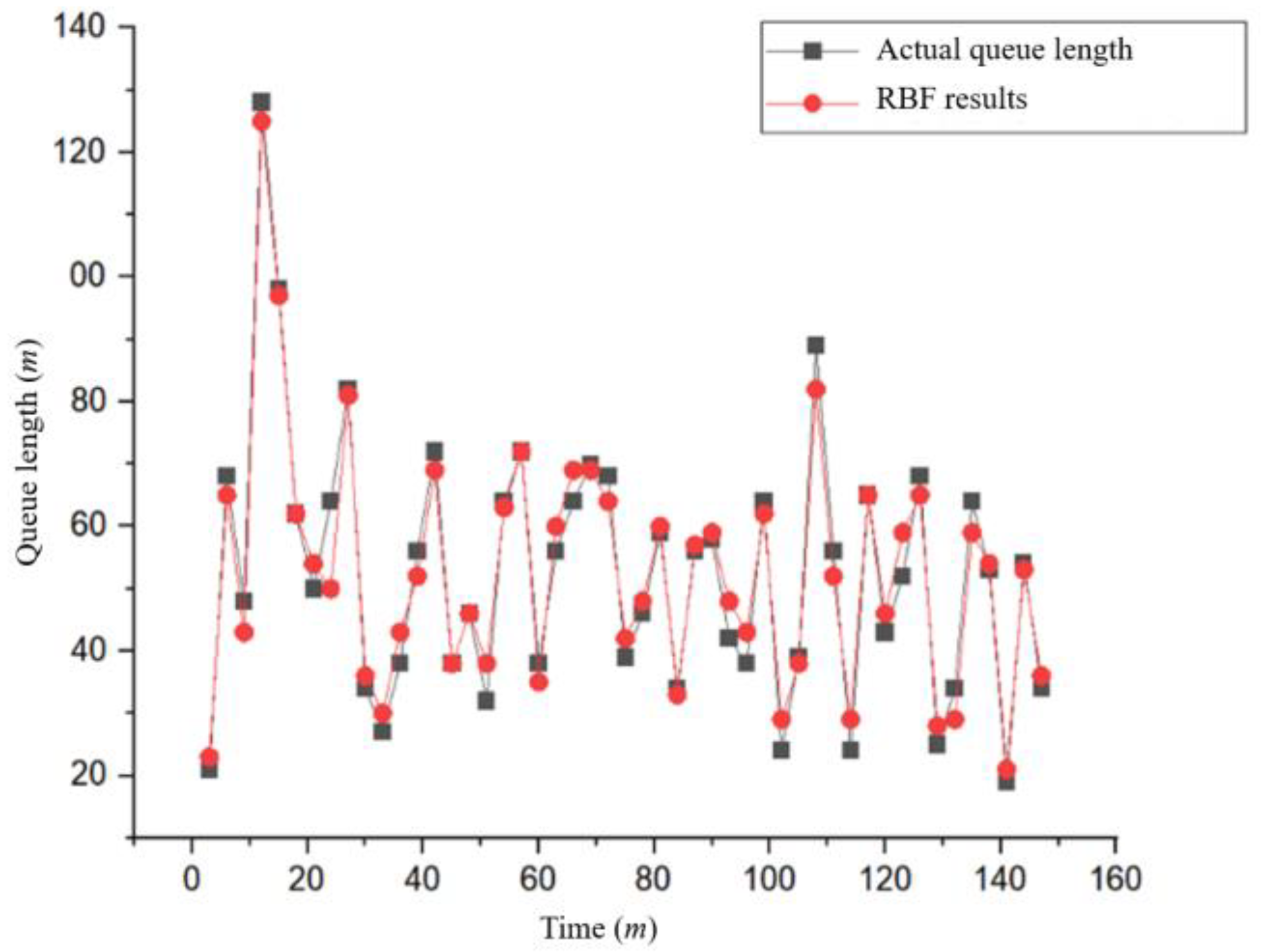
3.3.1. Estimation of Queue Length

Under the framework of vehicle–road–cloud integration, the queue length can be predicted through historical queue length information. A radial basis function (RBF) neural network [37] was established to estimate the queue length. The output of the hidden layer nodes is a linear combination of input vectors and is nonlinearly mapped to the output layer using an exponential function. The RBF neural network model can be established as:

$$y_k=\sum _{i=1}^n{w}_{ki}{e}^{w_i^{T}x+b_i}+{\theta }_k$$

(13)

where $y_k$ is the output of the k^th node in the output layer; $w_{ki}$ is the weight from the i^th node in the hidden layer to the k^th node in the output layer; $w_i$ and $b_i$ are the weight and bias of the i^th node in the hidden layer; $x$ is the input vector; ${\theta }_k$ is the threshold of the k^th node in the output layer.

Then, historical datasets, including traffic volume, average vehicle speed, and signal phase under unstable and dynamic traffic flow conditions and corresponding queue length data, were utilized to train the RBF neural network. By minimizing the difference between the predicted queue length and the actual queue length, the weights of the network were adjusted to optimize the accuracy of the prediction. After training, a parameterized function was obtained, as shown in Formula (14), which predicted the queue length based on real-time traffic volume, average speed, and signal phase.

$$L_q=f(Q_C,V_C,c_r)$$

(14)

where $L_q$ is the queue length; $Q_C$ is the traffic volume; $V_C$ is the average vehicle speed; $c_r$ is the duration of the red light time.

Finally, after real-time monitoring of the traffic volume, average speed, and signal phase, the trained RBF neural network model was used to calculate the queue length at the intersection.

3.3.2. Valid Traffic Signal Model

When the green light at the intersection turns on, if there is a long queue ahead of the connected vehicle, the vehicle needs to wait for the social vehicles ahead to pass through the intersection. That is to say, the connected vehicle can not pass through the intersection in an orderly manner until the queue dissipates. Thus, the actual time that can be used for vehicles passing through the intersection is less than the duration of green light time due to the additional signal spatiotemporal restricted zone, as shown in Figure 3. A valid traffic signal model was established to unite signal phase and queue length jointly.

Figure 3. Joint modeling diagram of signal phase and queue length.

The state of the traffic flow is relatively stable at the queue dissipation stage. The dissipation speed of the queue can be calculated based on the traffic flow wave theory:

$${\omega }^i=Q_c^i/({\rho }_c^i-{\rho }_d^i)$$

(15)

where i is the i^th intersection; ${\omega }^i$ is the dissipation speed of the traffic queue; $Q_c^i$ is the maximum traffic capacity; ${\rho }_c^i$ is the traffic density at the maximum capacity and ${\rho }_d^i$ is the density of congested traffic flow.

The dissipation time can be obtained from the queue length $L_q$ and the dissipation speed ${\omega }^i$.

$${\mathsf{\Delta }}_t=L_q^i/{\omega }^i$$

(16)

Define this time as the additional red light time ${\mathsf{\Delta }}_t$, which is the time when the main vehicle is not allowed to pass through the intersection after the green light is on.

The valid duration of the red light $q_r^i$ is the total time that the main vehicle can not pass through the intersection, so $q_r^i$ includes the additional red light time ${\mathsf{\Delta }}_t$ and the actual red light time $c_r$ of the basic signal. The cycle time $T^i$ is the sum of the valid duration of the red light $q_r^i$ and the valid green light duration $q_g^i$.

$$\left\{\begin{array}{c}{q}_r^i=c_r^i+{\mathsf{\Delta }}_t\\ q_r^i+q_g^i=T^i\end{array}\right.$$

(17)

By jointly modeling the signal phases and traffic queue, the valid traffic signal model $S^i\left(t\right)$ can be obtained:

$$S^i(t)=\left\{\begin{array}{l}1,T_0^i+(j-1)T^i+c_r^i+{\mathsf{\Delta }}_t<t<T_0^i+j{T}^i\\ 0,\mathrm{otherwisw}\end{array}\right.$$

(18)

where j is the j^th signal cycle at the i^th intersection. The time range of $(T_0^i+(j-1)T^i+c_r^i+{\mathsf{\Delta }}_t,T_0^i+j{T}^i)$ represents the j^th green light window. $S_i\left(t\right)=1$ indicates that the i^th intersection is in the j^th valid green light window and the main vehicle can pass through the i^th intersection; otherwise $S_i\left(t\right)=0$ indicates that the i^th intersection is in a valid red light window. $T_0^i$ is the initial signal offset for the i^th intersection.

The speed induction strategy for an isolated intersection is to calculate the most energy-efficient ecological speed based on the three scenarios of acceleration, deceleration, and stopping in the optimal energy consumption model within the next valid green light window.

3.4. Multi-Intersections-Based Eco-Approach and Departure Strategy (M-EAD)

Due to the spatiotemporal correlation between multiple traffic signals, the coupling relationship between the spatial position and signal phases needs to be considered at multi-intersections. However, The effect of speed control at multi-intersections is not “equal” to that of the “superposition” of I-EAD. Moreover, there is also a problem of balancing optimal travel time and energy consumption at multi-intersections. Aiming at breaking through the limitations of speed planning at isolated intersections, a two-stage optimization multi-intersections-based eco-approach and departure (M-EAD) strategy was proposed as shown in Figure 4: in the first stage, the efficient green light window was obtained under the constraints of vehicle dynamics and signal phases from Figure 4a to Figure 4b; in the second stage, the optimal vehicle speed trajectory satisfying travel time and energy consumption under the constraint of the efficient green light window was gained from Figure 4b to Figure 4c.

Figure 4. The framework of M-EAD: (a) feasible speed trajectories; (b) efficient green light window; (c) optimal vehicle speed trajectory.

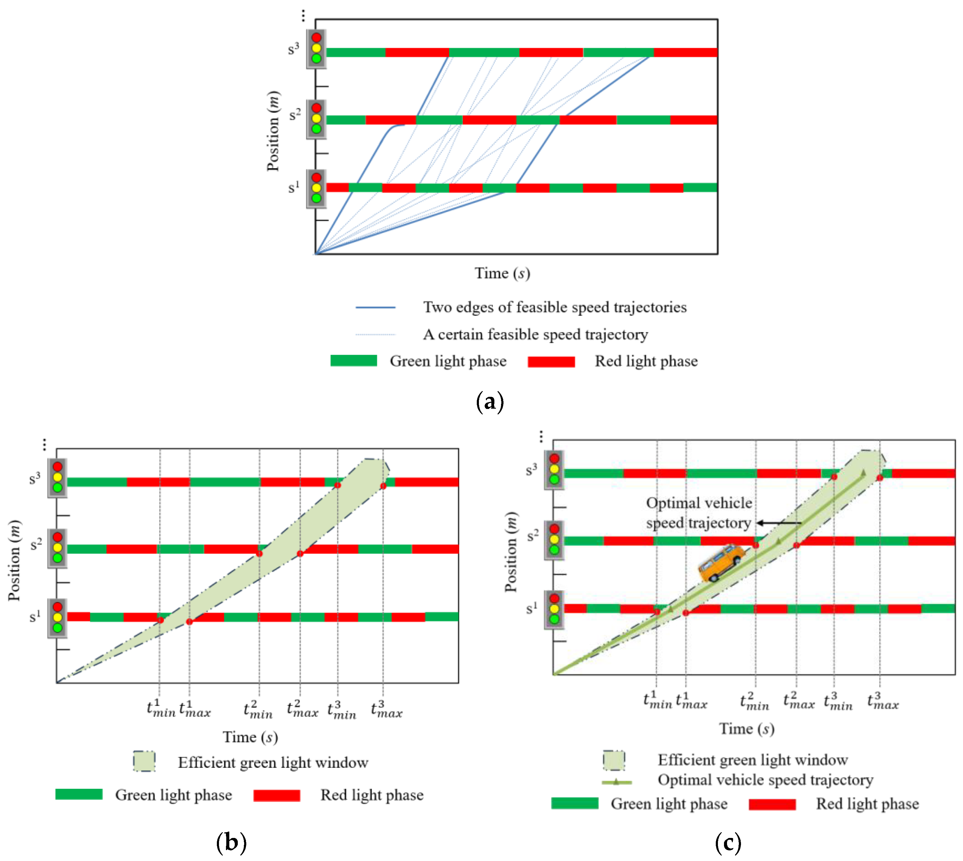
3.4.1. Efficient Green Light Window Model

There are multiple feasible green light windows at each intersection and coupling relationships of green light windows between adjacent intersections. The efficient green light window model was established based on directed graph theory. The efficient green light window planning problem was transformed into finding the shortest path in the directed graph [38].

The time range of a vehicle arriving at the intersection was calculated. The arrival time is influenced by two factors. The first factor is the dynamic characteristics of the vehicle. Vehicles can arrive within the maximum and minimum speed limitations. The shortest and longest arrival times based on the speed limitations are $t_{vmin}^i$ and $t_{vmax}^i$, respectively. The second factor is the valid green light time, which can be calculated and corrected based on Formula (18) due to signal phases, the current traffic conditions, and queue length. The shortest global travel time $t_{min}^i$ and longest global travel time $t_{max}^i$ of the vehicle at the i^th intersection can be predicted as follows:

$$\left\{\begin{array}{l}{t}_{min}^i=t_{min}^{i-1}+max(t_{\nu min}^i-(T_0^i+(j-1)T^i),c_r^i+\Delta t)\\ t_{max}^i=t_{max}^{i-1}+min(t_{\nu max}^i-(T_0^i+j{T}^i),c_r^i+\Delta t)\end{array}\right.$$

(19)

Simplify each intersection as a node and define the set $A^i$ as the set of feasible green window numbers that can be calculated by dividing the travel time by the signal cycle for the intersection $S_i$.

$$A^i=\left[\mathrm{ceil}\left({\displaystyle \frac{t_{min}^i-T_0^i}{T^i}}\right),\mathrm{ceil}\left({\displaystyle \frac{t_{max}^i-T_0^i}{T^i}}\right)\right]$$

(20)

where ceil is an integer-up function.

The solution of the directed graph is transformed into minimizing the sum of all feasible valid green window numbers $W^i$ for all nodes.

$$\begin{array}{c}\mathrm{Minimize}\\ {\left\{W^i\in A^i\right\}}_{i=1}^N\end{array}\sum _{i=1}^N W^i$$

(21)

The efficient green light window model can be transformed into a simple and classic shortest path problem, which has the characteristics of a dense graph with fewer nodes. Therefore, Floyd’s algorithm can be utilized to obtain an efficient green light window and time series in Formula (21). There are two kinds of possible shortest paths for any node m to n: directly from m to n and passing through several nodes k from m to n. When k = 0, there are no nodes between m and n, and the shortest path is the weight from m to n; When k ≥ 1, Floyd’s algorithm is a process of reducing weights by traversing nodes.

$$d_{mn}^k=\mathit{min}(d_{mn}^{k-1},d_{mk}^{k-1}+d_{kn}^{k-1})$$

(22)

where $d_{mn}^k$ represents the distance of the shortest path from node m to n.

3.4.2. Optimal Vehicle Speed Trajectory Model

The appropriate speed and acceleration for each moment for the optimal vehicle speed trajectory can be selected within the efficient green light window. The model integrates multiple objectives and constraints and requires comprehensive consideration of goals such as energy conservation and travel time reduction.

The deep reinforcement learning algorithm was proposed to solve the optimal velocity trajectory after discretization. The state space $x\left(t\right)=\left[v\right(t),T]$ is composed of the vehicle speed $v\left(t\right)$ and the global travel time $T$. The action space $u\left(t\right)=a\left(t\right)$ is the acceleration $a\left(t\right)$ of the vehicle and is the control variable of the optimization problem. The reward function consists of two parts: the first part is the objective function of reducing energy consumption, which is achieved by reducing the total input energy consumption of the electrical motor. According to Formula (11), the instantaneous energy consumption of an electric vehicle is affected by the speed $v\left(t\right)$ and acceleration $a\left(t\right)$. The second part is the objective function of reducing travel time. The weight factors ${\alpha }_1$ and ${\alpha }_2$ can balance and adjust the goals of energy conservation and travel time reduction. The reward function is shown in the following formula:

$$R_t={\alpha }_1{\int }_0^{T}P\left[u\left(t\right),x\left(t\right)\right]d_t+{\alpha }_{2}T\left[u\left(t\right),x\left(t\right)\right]$$

(23)

where $P\left[u\left(t\right),x\left(t\right)\right]$ is the instantaneous energy consumption of the electric vehicle.

The safe DQN (deep Q network) reinforcement learning algorithm with experience replay was used to optimize the speed trajectory. The CNN (convolutional neural network) that can effectively process spatial structure information was adopted to approximate the Q-learning function, and the $\mathsf{\epsilon }-\mathrm{greedy}$ strategy was used to achieve “development” and “exploration” in reinforcement learning [39].

The existing intelligent agent with state $x_t$ selects action $u_t$ through the $\mathsf{\epsilon }-\mathrm{greedy}$ strategy, executes it in the traffic environment, and obtains reward value $R_t$ and new state $x_{t+1}$ after observing the environment. Then, the experience matrix $(x_t,u_t,R_t,x_{t+1})$ is stored in the experience pool. During the training process, a small number of experience samples are randomly selected from the replay buffer, and the greedy factor is updated through the stochastic gradient descent algorithm. Repeat the process until the training is completed. The target Q value can be expressed as:

$$Q(x_{t+1},u_{t+1})=Q(x_t,u_t)+\alpha [R_{t+1}+\gamma \mathit{argmax}Q(x_t^{\prime },u_t^{\prime })-Q(x_t,u_t\left)\right]$$

(24)

where $\gamma \mathit{argmax}Q(x_t^{\prime },u_t^{\prime })$ represents the process that the state $x_t$ changes to the state $x_t^{\prime }$ after executing the action $u_t$ and the cumulative reward value generated by the best action $u_t^{\prime }$ after calculating the loss function. The learning rate $\alpha$ can control the convergence rate of the algorithm. The discount factor $\gamma \in [0,1]$ is a parameter to measure the relative importance of future rewards. The larger the value of $\gamma$ in the learning process, the more emphasis is placed on long-term rewards, while the smaller the value of $\gamma$, the more emphasis is placed on immediate rewards.

The relevant parameters setting for the study are as follows: learning rate $\alpha$ is 0.001, discount factor $\gamma$ is 0.99, the size of experience pool is 20,000, the sampling batch is 64, and $\mathsf{\epsilon }-$ greedy factor is 0.001. When adjusting the priority parameter of the simulation time, it is calculated each time step, with a total training time of 3600 s and 200 training iterations.

Constraint conditions are shown as Formulas (25)–(29). Formula (25) is a distance constraint used to solve the global travel time; Formula (26) is the constraint of the efficient green light window, where $t^i$ is the actual arrival time to reach the intersection $S_i$; Formula (27) represents the maximum and minimum speed constraints of the vehicle; Formula (28) represents the constraints on vehicle acceleration and deceleration; Formula (24) represents the initial state of the problem. The safe DQN algorithm [40] was proposed to determine the optimal speed trajectory, and interventions were adopted in the action output layer to ensure that they did not violate the constraints.

$$d={\int }_{t=0}^{T}v\left(t\right)dt$$

(25)

$$max(t_{min}^i,T_0^i+(W^i-1\left)T^i\right)\le t^i\le min(t_{max}^i,T_0^i+W^i{T}^i)$$

(26)

$${\nu }_{min}\le \nu (t)=\int a(t)dt\le {\nu }_{max}$$

(27)

$$a_{dmax}\le a\left(t\right)\le a_{amax}$$

(28)

$$v\left(0\right)=v_0, d\left(0\right)=0$$

(29)

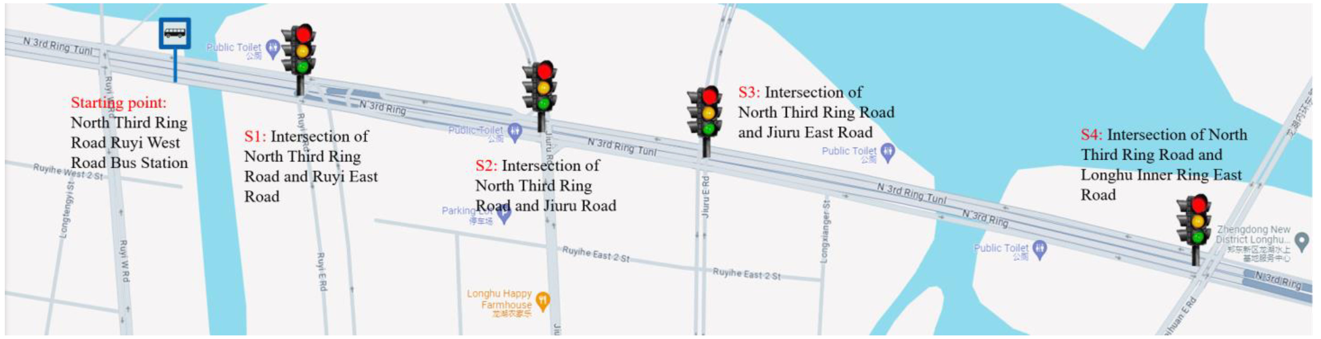
4. Simulation Results

The simulation background was based on the Autonomous Bus Line 1 of Zhengzhou Financial Island in Henan Province, China. There are four signalized intersections within the selected study area, as shown in Figure 5. The distance between each intersection and the starting point (the first bus stop), green light time, cycle time, traffic volume, and maximum and minimum speed limitations are shown in Table 1. Using Yutong’s autonomous bus as the main control vehicle, the relevant parameters of the vehicle are shown in Table 2. During the simulation process, the parameter values are: initial vehicle speed is 36 km/h; maximum speed is 50 km/h; minimum speed is 20 km/h; maximum acceleration is 2.5 m/s²; maximum deceleration is 3.0 m/s².

Figure 5. The simulation background and selected study area of the Autonomous Bus Line 1.

Table 1. Multi-intersections-related simulation parameters.

Intersection	Distance (m)	Greenlight Time (s)	Cycle Time (s)	Traffic Volume (veh/h)	Speed Limitations/km/h
					Maximum	Minimum
S1	325	45	90	750	60	20
S2	895	30	90	1056	60	20
S3	1300	45	90	978	60	20
S4	2400	38	90	1152	60	20

Table 2. Vehicle-related simulation parameters.

Parameter	Value	Parameter	Value
vehicle length (m)	12	frontal area (m2)	7.55
total weight (kg)	18,000	wind resistance coefficient	0.67
curb weight (kg)	10,650	rolling resistance coefficient	0.02
passengers/seats	79/29	conversion coefficient of rotating mass	1.04
rated power of motor (kW)	120	transmission ratio of the transmission system	6.33
peak power of motor (kW)	240	rolling radius of the wheel (m)	0.54
maximum torque of motor (Nm)	2800	wheelbase (m)	6
energy consumption per additional unit mass Ekg (Wh/km·kg)			0.161

The SUMO/Matlab/Simulink/Python joint simulation platform was built to verify the feasibility of I-EAD and M-EAD strategies. The software versions used are as follows: SUMO 1.16.0, Matlab R2021b, and Python 3.11.5. Simulink Automotive Dynamics Toolbox is integrated into Matlab software. A simulated road network was built using the real road environment of Autonomous Bus Line 1 in the SUMO traffic simulation software. The signal phase, traffic volume, and speed limitations at multi-intersections were set according to survey data in Table 1. I-EAD and M-EAD strategies were designed mainly in Python software. The traffic volume, the average vehicle speed, the duration of the red light time, and the queue length were recorded in SUMO as historical data, and then the RBF model and the valid traffic signal model were established in Python software to predict real-time queue length and determine the real-time additional signal spatiotemporal restricted zone by real-time data from SUMO simulation. The directed graph and the deep reinforcement learning algorithm were calculated in Python as well to solve the efficient green light window and the optimal vehicle speed trajectory. The energy consumption model was established in Matlab/Simulink by inputting parameters in Table 2. Moreover, the energy consumption of each simulation was also calculated in Matlab/Simulink. The TraCI (Traffic Control Interface) was used to achieve joint simulation of SUMO, Python, and Matlab/Simulink. The value of vehicle stata and signal information were obtained by TraCI.object.getvalue function and were assigned by TraCI.object.setvalue function.

4.1. Energy Consumption Model Results under Different Scenarios

According to the energy consumption model, different acceleration/deceleration/uniform time will result in different speed trajectories and corresponding energy consumption, as shown in Figure 6.

Figure 6. Energy consumption corresponds to time under different scenarios: (a) acceleration scenario; (b) deceleration scenario; (c) stopping scenario.

The relationship between energy consumption and acceleration time under the acceleration scenario is shown in Figure 6a. As the acceleration time increases, the acceleration value decreases gradually during the acceleration process, and at the same time, the total energy consumption corresponding to different speed trajectories shows a trend of first decreasing and then increasing. The minimum energy consumption is 0.417 kWh, with an acceleration time of 8 s and a corresponding acceleration value of 0.234 m/s².

The relationship between energy consumption and deceleration time in the deceleration scenario is shown in Figure 6b. As the deceleration time increases, the deceleration value increases gradually; at the same time, the total energy consumption shows a decreasing trend, with a minimum energy consumption of 0.107 kWh and a deceleration value of 0.111 m/s². This case illustrates that under the deceleration scenario, the lowest energy consumption will be obtained if the vehicle decelerates constantly to the minimum speed limitation from the current speed and passes through the intersection at the minimum speed limitation.

The relationship between energy consumption and uniform time in the stopping scenario is shown in Figure 6c. With the continuous increase of uniform time, the deceleration time decreases, and the deceleration value increases correspondingly. Meanwhile, total energy consumption shows a gradual increase. The minimum energy consumption is 0.036 kWh, with a uniform travel time of 0 s and a deceleration value of 0.1667 m/s². This case illustrates that when not meeting the conditions of acceleration and deceleration scenarios, the lowest energy consumption will be obtained if the vehicle decelerates at a constant deceleration value from the current speed to the speed of exactly 0 at the stopping line.

4.2. Estimation Result of Queue Length

A dataset was generated to estimate queue length using SUMO software. 90% of the data was selected Randomly as the training set, and 10% of the data was selected as the testing set. The TensorFlow package was used to build an RBF neural network model in the Python environment. The training set was trained to predict the queue length, and the predicted results were compared with the actual queue length, as shown in Figure 7, indicating that the RBF neural network still exhibits excellent performance in queue length prediction despite unstable traffic flow.

Figure 7. Estimation result of queue length by RBF neural network.

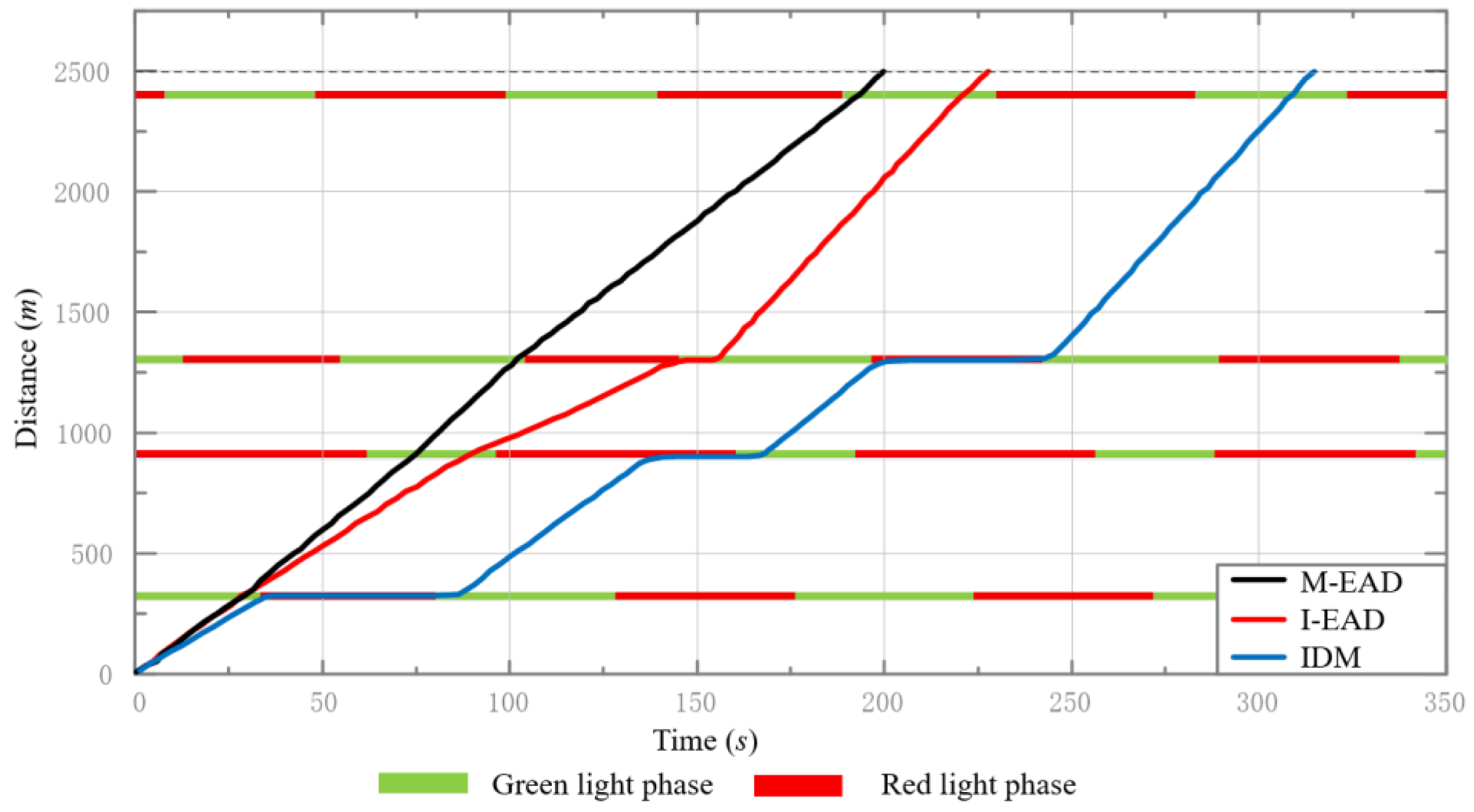
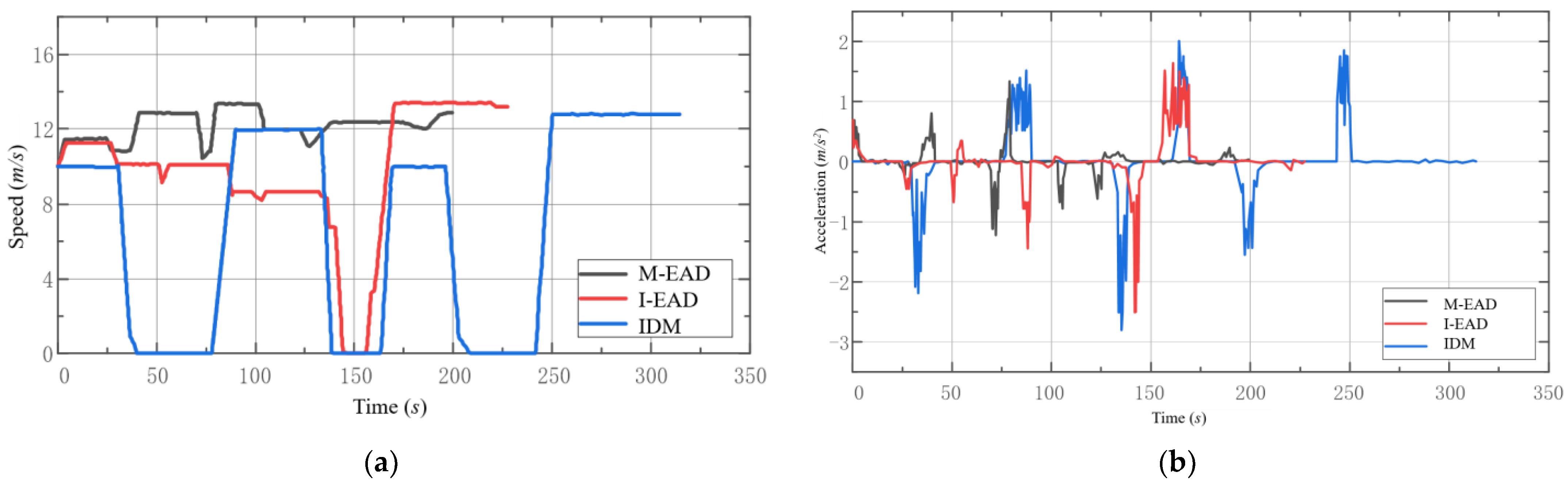
4.3. Comparison Results of Speed Planning Strategies

Comparative experiments were conducted to verify the effectiveness of the vehicle speed induction strategies proposed in this study. Travel energy consumption and travel time were compared under the same scenario and conditions, such as the same approach and departure time and the same starting point. Three strategies for vehicle speed planning were adopted:

• The intelligent driver model (IDM) mentioned in reference [41] was used as the basic method for simulation in the study. On the SUMO platform, an IDM car-following model could be used directly, simulating the process of drivers operating based on their experience without speed planning. By comprehensively considering factors such as safe distance between vehicles, speed difference, and expected speed, the corresponding acceleration was calculated to describe the driver’s behavior, thereby achieving an adaptive cruise control strategy and safe car-following model;
• The isolated-intersection-based eco-approach and departure (I-EAD) strategy was used for speed planning, and then the IDM strategy was used for the car-following process when the main vehicle was influenced by the preceding vehicle;
• The multi-intersections-based eco-approach and departure (M-EAD) strategy was used for speed planning, and then the IDM strategy was also used for the car-following process;

The simulation results of distance, speed, and acceleration/deceleration over time when using IDM, I-EAD, and M-EAD strategies are shown in Figure 8 and Figure 9.

Figure 8. Distance curve over time.

Figure 9. Kinematic variation curve over time: (a) speed variation curve; (b) acceleration variation curve.

Figure 8 shows that vehicles driving under the IDM strategy cannot obtain signal information from the downstream traffic lights in advance and cannot be guided in advance. There are stopping behaviors at the first, second, and third signalized intersections when encountering red lights. There is no doubt that travel time is the longest throughout the entire journey compared with the I-EAD and M-EAD strategies. Vehicles using the I-EAD strategy, compared to the IDM strategy, only experience a stop at the third intersection due to the consideration of queue length caused by the current red light phase, leading to a moderate travel time. Vehicles adopting the M-EAD global speed optimization strategy try their best efforts to pass through all intersections without stopping while considering the signal phase, queue length, kinematics, and dynamics constraints, resulting in the shortest travel time.

From Figure 9a,b, there is a longer acceleration/deceleration duration and a more significant speed fluctuation due to frequent acceleration and deceleration process when adopting the IDM strategy; vehicles stop at the third intersection using I-EAD strategy based on the valid traffic signal light model; there are no stopping phenomenon and intense acceleration/deceleration movements throughout the entire process when passing through four consecutive signalized intersections when using the M-EAD strategy. The preceding vehicle influences the acceleration fluctuations of I-EAD and M-EAD strategies.

As shown in Table 3, the I-EAD speed guidance strategy reduces energy consumption by 13.79% and travel time by 27.61% compared to the IDM strategy with multiple go-and-stop behavior. Compared with IDM and I-EAD strategies, the M-EAD strategy considering efficient green light windows reduces energy consumption by 21.94% and 9.45% and travel time by 36.51% and 12.29%, respectively. The M-EAD strategy has shown good optimization effects in energy conservation and efficient transportation.

Table 3. Simulation results comparison between three strategies.

Strategies	Travel Energy Consumption	Travel Time	Energy Consumption Reduction		Travel Time Reduction
			IDM	I-EAD	IDM	I-EAD
IDM	3.19 kwh	314.7 s	-	-	-	-
I-EAD	2.75 kwh	227.8 s	13.79%	-	27.61%	-
M-EAD	2.49 kwh	199.8 s	21.94%	9.45%	36.51%	12.29%

4.4. Random Traffic Scenario Verification

Although the above simulation results indicated that the M-EAD strategy had excellent improvement performance, it was the result of a single typical traffic scenario. It was a special scene chosen by the authors for the sake of visual effects and a better improvement effect to make the visualization results more obvious, which could not explain its average performance in random traffic scenarios. Therefore, 500 simulation experiments under random traffic scenarios were designed and conducted. A fixed signal was still adopted, and the initial signal phases and offset were generated randomly in these experiments.

The average energy consumption power and average travel time under a random traffic scenario were obtained, as shown in Figure 10 and Table 4. The I-EAD strategy reduces average travel energy consumption and average travel time by 9.10% and 15.78%, respectively, compared to the IDM strategy. Compared to IDM and I-EAD strategies, M-EAD reduces average travel energy consumption by 16.65% and 8.31%, and average travel time decreases by 26.33% and 12.53%, respectively. The above results illustrate that the M-EAD global green wave ecological speed planning strategy designed in this study for continuous signalized intersections has universal advantages both in typical and random traffic scenarios. At the same time, the optimization effect under a random traffic scenario is not completely consistent with the typical traffic scenario mentioned above, indicating that the random traffic environment influences the effectiveness of the strategy, but it shows overall good optimization results.

Figure 10. Simulation results under random traffic scenario between three strategies: (a) average travel energy consumption; (b) average travel time.

Table 4. Average reduction of energy consumption and travel time between the three strategies.

Strategy	Average Reduction
	Energy Consumption	Travel Time
I-EAD strategy compared to IDM strategy	9.10%	15.78%
M-EAD strategy compared to IDM strategy	16.65%	26.33%
M-EAD strategy compared to I-EAD strategy	8.31%	12.53%

5. Conclusions

With the rapid development of connected vehicle technology, vehicle–road–cloud integration has become the future development direction of autonomous vehicles. Compared with the speed guidance of vehicle-road collaboration, the speed guidance system based on vehicle–road–cloud integration can simultaneously optimize the speed of multiple signalized intersections and road sections under the unified monitoring of the cloud control center while avoiding the time delay caused by dedicated short-range communication between onboard units and roadside unit. The cloud control center’s powerful computing and multi-source information fusion capabilities can greatly accelerate computing speed, ensuring the provision of speed planning in real-time. In response to the reduction of energy consumption and traffic efficiency caused by intersection congestion, a green wave ecological global speed planning was investigated based on the vehicle–road–cloud integration system. The main conclusions and innovations are as follows:

• Previous scholars have mostly researched green wave speed induction strategies for fuel vehicles, using the fuel consumption model to construct fuel consumption optimization objective functions. With the development of the automotive vehicle industry, most connected autonomous vehicles are pure electric vehicles. Therefore, electric vehicles were selected as the research object. An instantaneous energy consumption model for electric vehicles using power balance equations was established, and the optimal consumption model was calculated using acceleration, deceleration, and stopping scenarios.
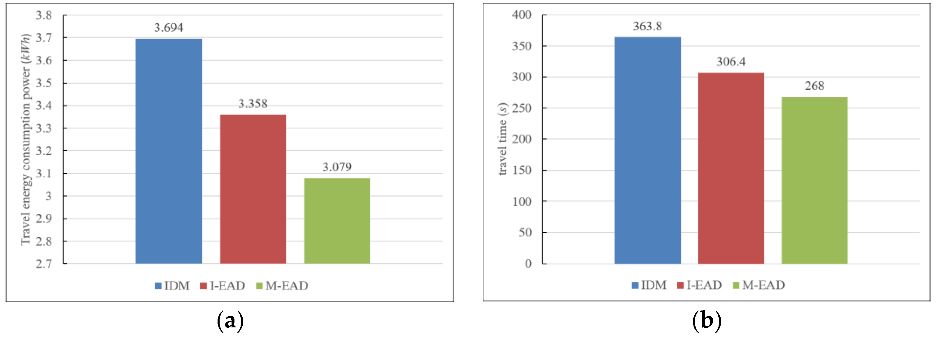
• Previous scholars often only considered signal constraints and did not take into account the impact of the queue length of social vehicles. A radial basis function neural network model and a valid traffic signal model were proposed to estimate the effect of queue length of traffic flow during the green light time at signalized intersections. The I-EAD strategy reduces average energy consumption by 9.10% and average travel time by 15.78%, respectively, compared to the IDM model.
• A two-stage, multi-intersections-based eco-approach and departure strategy was established to solve the problem of an efficient green light window and the optimal vehicle speed trajectory. Compared to IDM and I-EAD strategies, the M-EAD strategy reduces average travel energy consumption by 16.65% and 8.31% and the average travel time by 26.33% and 12.53%, respectively.

Although strict assumptions have been clearly stated in the study, such as ignoring the influence of non-connected vehicles and communication delays, these limitations may affect the generalizability of the findings in more complex traffic scenarios. While theoretically robust, the proposed strategies may face challenges in real-world implementation due to the complexities of integrating vehicle–road–cloud systems at a large scale. Future research should include real-world trials in diverse traffic environments of different urban settings to validate the simulation results.

References

1. Simchon, L.; Rabinovici, R. Real-Time Implementation of Green Light Optimal Speed Advisory for Electric Vehicles. Vehicles 2020, 2, 35–54. [Google Scholar] [CrossRef]
2. Li, K.; Dai, Y.; Li, S.; Bian, M. State-of-the-art and technical trends of intelligent and connected vehicles. J. Automot. Saf. Energy 2017, 8, 1. [Google Scholar]
3. Lin, H.; Liu, Y.; Li, S.; Qu, X. Research progress on key technologies of vehicle road collaboration system. J. South China Univ. Technol. (Nat. Sci. Ed.) 2023, 51, 46–67. [Google Scholar]
4. Cheng, Z.Q.; Dai, Q.; Li, S.Y.; Teruko, M.; Alexander, H. GSRFormer: Grounded Situation Recognition Transformer with Alternate Semantic Attention Refinement. In Proceedings of the MM ‘22: The 30th ACM International Conference on Multimedia, Portugal, Lisbon, 10–14 October 2022. [Google Scholar]
5. Alalewi, A.; Dayoub, I.; Cherkaoui, S. On 5G-V2X Use Cases and Enabling Technologies: A Comprehensive Survey. IEEE Access 2021, 9, 107710–107737. [Google Scholar] [CrossRef]
6. Amendola, D.; Cordeschi, N.; Bai, F.; Ji, Y.S.; Yan, S.; Zhuang, W.H. Guest Editorial Special Issue on 5G/6G Precise Positioning on Cooperative Intelligent Transportation Systems (C-ITS) and Connected Automated Vehicles (CAV)-Part I. IEEE J. Sel. Areas Commun. 2023, 41, 3713–3718. [Google Scholar] [CrossRef]
7. Kuru, K.; Khan, W. A Framework for the Synergistic Integration of Fully Autonomous Ground Vehicles With Smart City. IEEE Access 2021, 9, 923–948. [Google Scholar] [CrossRef]
8. Li, K.; Li, J.; Chang, X.; Gao, B.; Xu, Q.; Li, S. Principles and typical applications of cloud control system for intelligent and connected vehicles. J. Automot. Saf. Energy 2020, 11, 261. [Google Scholar]
9. Arthurs, P.; Gillam, L.; Krause, P.; Wang, N.; Halder, K.; Mouzakitis, A. A Taxonomy and Survey of Edge Cloud Computing for Intelligent Transportation Systems and Connected Vehicles. IEEE Trans. Intell. Transp. Syst. 2022, 23, 6206–6221. [Google Scholar] [CrossRef]
10. Kodi, J.H.; Kidando, E.; Sando, T.; Alluri, P. Estimating the Mobility Benefits of Adaptive Signal Control Technology Using a Bayesian Switch-Point Regression Model. J. Transp. Eng. A Syst. 2022, 148, 5. [Google Scholar] [CrossRef]
11. Shams, A.; Mahmud, S.; Day, C.M. Comparison of Flow- and Bandwidth-Based Methods of Traffic Signal Offset Optimization. J. Transp. Eng. A Syst. 2023, 149, 5. [Google Scholar] [CrossRef]
12. Yang, L.; Zhao, X.; Wu, G.; Xu, Z.; Matthew, B.; Hui, F.; Hao, P.; Han, M.; Zhao, Z.; Fang, S.; et al. Review on connected and automated vehicles based cooperative eco-driving strategies. J. Traffic Transp. Eng. 2020, 20, 58–72. [Google Scholar]
13. HomChaudhuri, B.; Vahidi, A.; Pisu, P. Fast model predictive control-based fuel efficient control strategy for a group of connected vehicles in urban road conditions. IEEE Trans. Control Syst. Technol. 2017, 25, 760–767. [Google Scholar] [CrossRef]
14. HomChaudhuri, B.; Vahidi, A.; Pisu, P. A Fuel Economic Model Predictive Control Strategy for a Group of Connected Vehicles in Urban Roads. In Proceedings of the American Control Conference, Chicago, IL, USA, 1–3 July 2015. [Google Scholar]
15. Ala, M.V.; Yang, H.; Rakha, H. Modeling evaluation of eco–cooperative adaptive cruise control in vicinity of signalized intersections. Transp. Res. Rec. 2016, 2559, 108–119. [Google Scholar] [CrossRef]
16. Yang, H.; Rakha, H.; Ala, M.V. Eco-cooperative adaptive cruise control at signalized intersections considering queue effects. IEEE Trans. Intell. Transp. Syst. 2016, 18, 1575–1585. [Google Scholar] [CrossRef]
17. Altan, O.D.; Wu, G.; Barth, M.J.; Boriboonsomsin, K.; Stark, J.A. GlidePath: Eco-friendly automated approach and departure at signalized intersections. IEEE Trans. Intell. Veh. 2017, 2, 266–277. [Google Scholar] [CrossRef]
18. Ye, F.; Hao, P.; Qi, X.; Wu, G.; Boriboonsomsin, K.; Barth, M. Prediction-based eco-approach and departure at signalized intersections with speed forecasting on preceding vehicles. IEEE Trans. Intell. Transp. Syst. 2018, 20, 1378–1389. [Google Scholar] [CrossRef]
19. Kari, D.; Wu, G.; Barth, M.J. Eco-friendly freight signal priority using connected vehicle technology: A multi-agent systems approach. In Proceedings of the IEEE Intelligent Vehicles Symposium (IV), Dearborn, MI, USA, 8–11 June 2014. [Google Scholar]
20. Wu, W.; Huang, L.; Du, R. Simultaneous optimization of vehicle arrival time and signal timings within a connected vehicle environment. Sensors 2019, 20, 191. [Google Scholar] [CrossRef]
21. Liu, B.; Sun, C.; Wang, B.; Sun, F. Adaptive speed planning of connected and automated vehicles using multi-light trained deep reinforcement learning. IEEE Trans. Veh. Technol. 2021, 71, 3533–3546. [Google Scholar] [CrossRef]
22. Wang, Q.Z.; Gong, Y.B.; Yang, X.F. Connected automated vehicle trajectory optimization along signalized arterial: A decentralized approach under mixed traffic environment. Transp. Res. Part. C Emerg. Technol. 2022, 145, 103918. [Google Scholar] [CrossRef]
23. Talukder, M.A.S.; Lidbe, A.D.; Tedla, E.G.; Hainen, A.M.; Atkison, T. Trajectory-Based Signal Control in Mixed Connected Vehicle Environments. J. Transp. Eng. A Syst. 2021, 147, 5. [Google Scholar] [CrossRef]
24. Shams, A.; Day, C.M. Advanced Gap Seeking Logic for Actuated Signal Control Using Vehicle Trajectory Data: Proof of Concept. Transp. Res. Rec. 2023, 2677, 610–623. [Google Scholar] [CrossRef]
25. Dong, H.; Zhuang, W.; Chen, B.; Yin, G.; Wang, Y. Enhanced eco-approach control of connected electric vehicles at signalized intersection with queue discharge prediction. IEEE Trans. Veh. Technol. 2021, 70, 5457–5469. [Google Scholar] [CrossRef]
26. Zhang, C.; Len, J.; Wang, B.; Sun, C.; Zhou, X. An Eco-Driving Method with Queue Length Estimation for Connected Vehicles. Trans. Beijing Inst. Technol. 2022, 42, 1256–1263. [Google Scholar]
27. Chen, Z.; Zhang, J.; Xiong, S.; Su, Z.; Hu, J.; Wu, C. A Review on Research Status and Trends of Eco-driving on Intelligent Connected Vehicles. J. Transp. Inf. Saf. 2022, 40, 13–25. [Google Scholar]
28. Bautista-Montesano, R.; Galluzzi, R.; Mo, Z.B.; Fu, Y.J.; Bustamante-Bello, R.; Di, X. Longitudinal Control Strategy for Connected Electric Vehicle with Regenerative Braking in Eco-Approach and Departure. Appl. Sci. 2023, 13, 5089. [Google Scholar] [CrossRef]
29. Jin, H.; Niu, R. Economic Speed Planning Based on A-Star Algorithm for Intelligent Vehicle in Traffic Light Intersection. Trans. Beijing Inst. Technol. 2023, 43, 595–601. [Google Scholar]
30. Meng, Z.; Qiu, Z. A Study of Eco-driving Strategy at Signalized Intersections. J. Transp. Inf. Saf. 2018, 36, 76–84+92. [Google Scholar]
31. Liu, H.; Kurzhanskiy, A.A.; Hong, W.S.; Lu, X.Y. Integrating vehicle trajectory planning and arterial traffic management to facilitate eco-approach and departure deployment. J. Intell. Transp. Syst. 2024. [Google Scholar] [CrossRef]
32. Dong, H.X.; Zhuang, W.C.; Wu, G.Y.; Li, Z.J.; Yin, G.D.; Song, Z.Y. Overtaking-Enabled Eco-Approach Control at Signalized Intersections for Connected and Automated Vehicles. IEEE Trans. Intell. Transp. Syst. 2024, 25, 4527–4539. [Google Scholar] [CrossRef]
33. Goyal, V. Development and Validation of Dynamic Programming Algorithm for Eco Approach and Departure. Master’s Thesis, Michigan Technological University, Houghton, MI, USA, 2021. [Google Scholar]
34. Yang, J.S.; Zhao, D.Z.; Jiang, J.J.; Lan, J.L.; Mason, B.; Tian, D.X.; Li, L. A Less-Disturbed Ecological Driving Strategy for Connected and Automated Vehicles. IEEE Trans. Intell. Transp. Syst. 2023, 8, 413–424. [Google Scholar] [CrossRef]
35. Han, J.H.; Rios-Torres, J. Fast Analytical Solver for Fuel-Optimal Speed Trajectory of Connected and/or Automated Vehicles. IEEE Trans. Control Syst. Technol. 2023, 31, 2714–2727. [Google Scholar] [CrossRef]
36. Rakha, H.A.; Kamalanathsharma, R.K.; Ahn, K. AERIS: Eco-Vehicle Speed Control at Signalized Intersections Using I2V Communication; Joint Program Office for Intelligent Transportation Systems: Washington, DC, USA, 2012. [Google Scholar]
37. Wang, X.; Shao, H. The Theory of RBF Neural Network and Its Application in Control. Inf. Control 1997, 26, 272–284. [Google Scholar]
38. Dong, H. Dynamic Optimization of Ecological Driving Speed For Intelligent and Connected Vehicle at Signalized Intersections. Ph.D. Thesis, Southeast University, Nanjing, China, August 2022. [Google Scholar]
39. Efroni, Y.; Tomar, M.; Ghavamzadeh, M. Multi-step Greedy Policies in Model-Free Deep Reinforcement Learning. In Proceedings of the ICLR 2020 Conference, Yasyabeba, Ethiopia, 30 April 2020. [Google Scholar]
40. Zhang, Q.; Miao, J.; Zhang, Z.; Yu, F.; Fu, F.; Wu, T. Energy-Efficient Video Streaming in UAV-Enabled Wireless Networks: A Safe-DQN Approach. In Proceedings of the GLOBECOM 2020—2020 IEEE Global Communications Conference, Taipei, Taiwan, 7–11 December 2020. [Google Scholar]
41. Sun, C.; Guanetti, J.; Borrelli, F.; Moura, S. Optimal Eco-Driving Control of Connected and Autonomous Vehicles Through Signalized Intersections. IEEE Internet Things J. 2020, 7, 3759–3773. [Google Scholar] [CrossRef]
Disclaimer/Publisher’s Note: The statements, opinions and data contained in all publications are solely those of the individual author(s) and contributor(s) and not of MDPI and/or the editor(s). MDPI and/or the editor(s) disclaim responsibility for any injury to people or property resulting from any ideas, methods, instructions or products referred to in the content.
Article Metrics
Citations
Article Access Statistics
Multiple requests from the same IP address are counted as one view.