Article

Global Low-Complexity Fault-Tolerant Control for Pure-Feedback Systems with Sensor Faults

1
Aviation Engineering School, Air Force Engineering University, Xi’an 710051, China
2
Department of Teaching and Research, Unit 93682 of the PLA, Beijing 101300, China
*
Authors to whom correspondence should be addressed.
Electronics 2024, 13(16), 3166; https://doi.org/10.3390/electronics13163166
Submission received: 26 June 2024 / Revised: 5 August 2024 / Accepted: 6 August 2024 / Published: 10 August 2024
(This article belongs to the Section Systems & Control Engineering)

Abstract

:
A low-complexity global fault-tolerant control method is proposed to solve the tracking problem of uncertain pure-feedback systems in the presence of sensor faults. First, a novel modeling approach is introduced to reconstruct the non-affine term, which removes the restriction that the non-affine function must be differentiable. Second, a novel nonlinear mapping based on inverse-tangent function is utilized in the controller design such that the control parameters are free from initial values of states compared to the traditional prescribed performance control methods, resulting in global fault-tolerant control of pure-feedback systems under sensor and actuator faults. Furthermore, the designed global controller is low-complexity in the sense that no time derivatives of system signals are involved in the controller, and no neural networks or fuzzy logic systems are used, though unknown nonlinearities are present in the considered systems, and the control parameters are allowed to be arbitrary positive constants. Finally, the proposed method is applied to numerical and tailless fly-wing UAV examples, which fully demonstrates the effectiveness of the proposed method.

1. Introduction

In recent years, numerous significant control techniques have been developed to address the tracking challenges of strict-feedback systems, as mentioned in [1,2,3]. However, pure-feedback systems have garnered increasing interest due to their extensive application potential. The domain of pure-feedback systems has seen a proliferation of research, with notable contributions including adaptive fuzzy control approaches [4,5,6,7,8], neural network-based control strategies [9,10,11], and robust control methodologies [12]. For example, Cheng et al. [13] proposed a neural-adaptive tracking control scheme to tackle the tracking control issue in uncertain pure-feedback nonlinear systems under dynamic constraints. Similarly, an adaptive barrier Lyapunov-function-based control scheme was proposed in reference [14] to realize asymptotic tracking performance for pure-feedback systems with full state constraints. In addressing the control dilemmas of nonlinear non-affine pure-feedback systems marred by unknown time delays and backlash-like hysteresis, Zhu et al. [15] proposed a novel control approach that integrates command filtered feedback with adaptive output, supported by the capabilities of extreme learning machines. To solve the explosion of complexity and potential control singularity that existed in the traditional adaptive backstepping controllers, reference [16] proposed a novel constructive identification and adaptive control method for pure-feedback systems, and Jia et al. designed a non-overshooting controller for nonlinear pure-feedback systems in reference [17]. Unfortunately, the aforementioned studies have employed the mean value theorem to reframe the pure-feedback systems into strict-feedback systems. Therefore, those methods cannot be applied the pure-feedback systems whose non-affine function is non-differentiable. To circumvent this limitation, Liu et al. [18] and Liu et al. [19] proposed adaptive control schemes that employ the Intermediate Value Theorem to reconstruct non-affine functions. After that, Zuo et al. [20] designed a neural-adaptive control strategy for the systems whose non-affine functions are not continuous concerning control variables or input. It is crucial to acknowledge that the aforementioned methodologies are not suitable for pure-feedback systems subject to sensor faults.
Given the potential for abrupt failures in diverse system elements like actuators, sensors, and processing units, research into ensuring fault tolerance and sustained functionality is especially crucial for systems where safety is paramount [21]. The presence of multiple sensor failures, which leads to inaccurate measurement of all system states, significantly degrades the operational efficiency of the system. Hence, the investigations on fault accommodation and performance maintenance have great theoretical and practical significance. A variety of sensor fault-tolerant techniques have been developed [22,23,24,25,26,27]. Among them, Ma et al. [23] introduced an adaptive control method through barrier Lyapunov function for systems under state constraints, ensuring finite-time error convergence. Huang et al. [27] proposed an adaptive neural control approach for multi-input and multi-output systems, which has pure-feedback form and time-varying asymmetric output constraints. Concurrently, the design of controllers must account for potential actuator failures, which can lead to system errors, reduced reliability, and even user harm. Bali et al. [28] presented a control approach that is both adaptive and fault-tolerant, specifically tailored for stochastic pure-feedback systems, utilizing radial basis function neural networks (RBFNN) to estimate uncertain nonlinearities while addressing both sensor and actuator faults. Jiang et al. [29] developed a decentralized adaptive security control mechanism for nonlinear pure-feedback multi-agent systems that switch asynchronously, which is robust against both sensor attacks and actuator malfunctions. An adaptive fault-tolerant control method for pure-feedback systems under actuator and sensor faults was proposed in reference [30], which guarantees that the system state does not violate bound boundaries. However, the controllers designed in the mentioned literature are still based on the restraint that the non-affine function must satisfy the differentiability condition. Moreover, the system also needs to satisfy the initial value condition, which limits the application of the existing control schemes. Furthermore, it is still an open problem that design the global control method for pure-feedback systems under sensor faults while guaranteeing the performance of the system.
Motivated by the above analysis, a global fault-tolerant control method for the pure-feedback systems with sensor faults and actuator faults is presented, in which the parameters of the controller are free from the initial conditions of the system. The principal innovations of this article are encapsulated below.
(1) The non-affine nonlinearities of the system are transformed into a novel strict-feedback form, which removes the requirement that the non-affine function must satisfy the differentiability condition. As a result, a global tracking controller is first achieved for the systems in pure-feedback form, whose non-affine nonlinearities are non-differentiable;
(2) In contrast to all the methods on pure-feedback systems, the problems of sensor faults and actuator faults are considered and solved by a novel global controller, which is designed based on twice state transformations using barrier functions and anti-barrier functions, i.e., arc tan · ;
(3) In contrast to the traditional prescribed performance control methods, the designed global controller is low-complexity in the sense that only state errors are involved in the controller, though unknown nonlinearities are present in the considered systems, and the control parameters can be arbitrary positive constants.

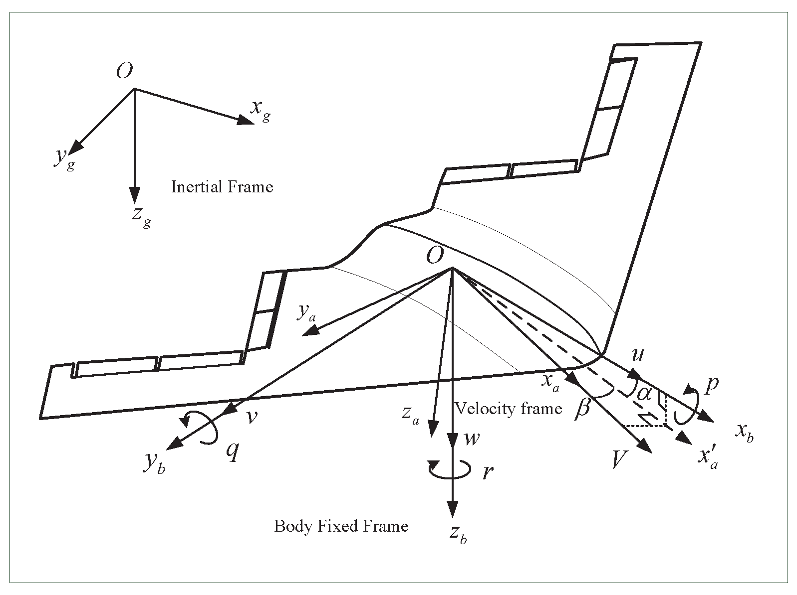
2. Problem Formulation and Preliminaries

The uncertain non-affine pure-feedback system is considered
ϱ ˙ i = f i ( ϱ ¯ i , ϱ i + 1 ) + Δ i ( t ) ϱ ˙ n = f n ( ϱ , u ) + Δ n ( t ) y = ϱ 1
where ϱ ¯ i = [ ϱ 1 , ϱ 2 , , ϱ i ] T , i = 1 , , n denotes the available state vector; y R and u R denote, respectively, the system control output and input; f i ( · ) is the unknown non-affine functions; z R -dimensional tracking error; Δ i ( t ) is the unknown bounded perturbation of the system.
Since non-affine functions are not differentiable, a more extensive functional model of the nonlinear system is presented, defining F i ( ϱ ¯ i , ϱ i + 1 ) = f i ( ϱ ¯ i , ϱ i + 1 ) f i ( ϱ ¯ i , 0 ) , wherein there is no need to require that f i ( ϱ ¯ i , ϱ i + 1 ) be continuously differentiable and f i ( ϱ ¯ i , 0 ) is continuous.
As a result of sensor malfunctions, the states of the system post-failure can be derived by employing alternative strategies.
Due to the sensor faults, the original states of the system (1) are no longer accessible. Then, the post-fault system states can be obtained from
ϱ i ( M ) = χ i ( t ) ϱ i + ς i ( t )
where ϱ i ( M ) represents the state measured by sensors, ς i ( t ) is the representation of additive sensor faults, χ i ( t ) is the multiplicative sensor faults that could magnify (when χ i ( t ) > 1 ) or compress (when 1 > χ i ( t ) > 0 ) the amplitude of ϱ i .
As discussed by Zhou et al. [31], the actuator fault containing the gain fault and bias fault can be expressed as follows:
u = γ ( t ) u a + δ ( t )
where γ ( t ) is the “health of indicator” and δ ( t ) denotes the bounded time-varying bias fault. It is assumed that γ ( t ) ( 0 , 1 ] .
The intention of this article is to propose a low-complexity global fault-tolerant control scheme for systems with sensor and actuator faults, such that the tracking error x 1 y d recovered into a region of arbitrarily small, and ensure that all the closed-loop signals are globally consistent and eventually bounded.
Assumption 1. 
For all x, and u, there exist constants i , υ i , i , υ i , such that
i ϱ i + 1 + υ i F i ( ϱ ¯ i , ϱ i + 1 ) ϱ i + 1 0 i ϱ i + 1 + υ i F i ( ϱ ¯ i , ϱ i + 1 ) ϱ i + 1 < 0
where i > 0 and i > 0 , i = 1 , 2 , , n .
Remark 1. 
The non-affine functions F i ( ϱ ¯ i , ϱ i + 1 ) is defined by f i ( ϱ ¯ i , ϱ i + 1 ) , and it can be seen from Assumption 1 that f i ( ϱ ¯ i , ϱ i + 1 ) are not required to be differentiable. Therefore, the restriction that f i ( ϱ ¯ i , ϱ i + 1 ) must be differentiable is removed.
Assumption 2. 
Let the desired trajectory be denoted as y d , with the assumption that y d , y ˙ d are continuously bounded.

3. Controller Design

In the following discussion, a low-complexity controller is going to be presented for systems with non-affine pure-feedback dynamics as depicted by Equation (1). Before that, a different state transformation method is proposed
z i = 1 ϖ i ( t ) arctan ( ϱ i ( M ) α i 1 ) , i = 1 , , n
where α 0 = y d , ϖ i ( t ) is selected by the designer according to the desired speed of tracking error convergence. In this paper, let ϖ i ( t ) = ( 1 ρ i ) e σ i t + ρ i , 0 < ρ i < 1 , σ i > 0 , and ρ i , σ i are positive constants for i = 1 , , n . Then, they satisfy 0 < ρ i ϖ i t 1 , ϖ ˙ i t ϖ * with ϖ * being positive constant.
Then, the following virtual and actual control signals are designed as follows
α i = κ i tan ( z i ) , i = 1 , , n 1
u a = κ n tan ( z n )
where κ i , i = 1 , , n are positive constants that can be arbitrarily selected by the designer.
Remark 2. 
From (5)–(7), it is crucial to point out that both the virtual and the actual control law are only the function of state errors without using any knowledge of system nonlinearities, which means the designed controller is model-free. Furthermore, the necessity of setting initial conditions, a common prerequisite in existing barrier function-based controllers, has been eliminated in this study, which is attributed to the use of arctan ( · ) in the barrier function-based controller design presented here.

4. Stability Analysis

The primary results of this research are now delineated.
Theorem 1. 
Consider the pure-feedback systems (1) under Assumptions 1 and 2, the virtual control signals (6), and the actual control law (7). Subsequently, the following properties are shown.
(1) All signals within the closed-loop system are guaranteed to remain bounded.
(2) The tracking performance satisfies ϱ 1 ( M ) y d Y M , for t > 0 , where Y M = tan ϖ 1 t π 2 .
Proof of Theorem 1. 
From the (5), it can be shown that z i ( 0 ) < π 2 , There is an unknown constant M 0 such that z i ( 0 ) < M 0 < π 2 for i = 1 , , n . It is useful to define the error vector z = [ z 1 , , z n ] T , and the following invariant set Ω 0
Ω 0 = [ M z , M z ] × × [ M z , M z ] n t i m e s
where M z = max i = 1 , , n { M 0 , arctan c i 4 } , and the value of c i 4 will be given later.
It is clear that 0 < M z < π 2 holds and z i ( 0 ) Ω 0 , i = 1 , , n . Defined z max ( t ) = max i = 1 , , n { z i ( t ) } . There are two cases for z max to be considered. Case (1) z max < M 0 holds for t > 0 such that z i ( t ) Ω 0 for t > 0 . Case (2) A time instance t M can be identified, defined as t M = inf { t | z max ( t ) = M 0 , t 0 } , where t M is strictly positive and represents the initial occurrence when the maximum system response z max ( t ) attains the threshold M 0 . For the interval 0 t t M , it is inherently true that each z i ( t ) Ω 0 remains within the predefined domain Ω 0 . Therefore, we are going to focus on proving that z i ( t ) Ω 0 for t [ t M , ) .
It should be pointed out that for t [ t M , ) , we have
ϖ i ( t ) ϖ i ( t M ) < 1 , i = 1 , , n
which will facilitate the subsequent analytical process.
Define the following open set
Ω z = ( π 2 , π 2 ) × × ( π 2 , π 2 ) n t i m e s
Then, we have Ω 0 Ω z and z i ( t ) Ω 0 implies
π 2 < z i ( t ) < π 2
Next, z i ( t ) Ω 0 for t [ t M , ) will be proved using (10) and (11).
From (5), we obtain
ϱ i ( M ) = tan ( ϖ i z i ) + α i 1 , i = 1 , , n 1 ϱ n ( M ) = tan ( ϖ n z n ) + α n 1
From (12), we have that ϱ i ( M ) is a continuous function of k i , z i , α i 1 , where k i and α i 1 are time-varying bounded functions. we can make a similar analysis for ϱ i + 1 ( M ) .
Step i , i = 1 , , n : The derivative of z i is
z ˙ i = ϖ ˙ i ϖ i 2 arctan ( ϱ i ( M ) α i 1 ) + ϱ ˙ i ( M ) α ˙ i 1 ϖ i ( 1 + tan 2 ( ϖ i z i ) )
The following positive definite functions candidates are considered:
V z i = 1 2 tan 2 ( z i )
The derivative of V z i is
V ˙ z i = tan ( z i ) cos 2 ( z i ) z ˙ i = tan ( z i ) cos 2 ( z i ) ϖ ˙ i ϖ i 2 arc tan ( ϱ i ( M ) α i 1 ) + ϱ ˙ i ( M ) α ˙ i 1 ϖ i ( 1 + tan 2 ( ϖ i z i ) ) = tan ( z i ) cos 2 ( z i ) ϖ ˙ i ϖ i 2 arc tan ( ϱ i ( M ) α i 1 ) + μ ˙ i ϱ i + μ i ϱ ˙ i + ς ˙ i α ˙ i 1 ϖ i ( 1 + tan 2 ( ϖ i z i ) ) = tan ( z i ) cos 2 ( z i ) ϖ ˙ i ϖ i z i + μ i ( F i ( ϱ i , ϱ i + 1 ) + f i ( ϱ i , 0 ) ) + μ ˙ i ϱ i + ς ˙ i + d i α ˙ i 1 ϖ i ( 1 + tan 2 ( ϖ i z i ) )
g i 0 ( ϱ ¯ i + 1 ) , g i 1 ( ϱ ¯ i + 1 ) is defined as follows:
g i 0 ( ϱ ¯ i + 1 ) = 2 ϱ i + 1 ϱ i + 1 2 + 0.25 ( F i ( ϱ i , ϱ i + 1 ) υ i ) g i 1 ( ϱ ¯ i + 1 ) = 2 ϱ i + 1 ϱ i + 1 2 + 0.25 ( F i ( ϱ i , ϱ i + 1 ) υ i )
From (4) and (16), g i 0 ( ϱ ¯ i + 1 ) i for ϱ i > 0.5 and g i 1 ( ϱ ¯ i + 1 ) i for ϱ i < 0.5 . The following inequation can be obtained
i ϱ i + 1 + υ i F i ( ϱ ¯ i , ϱ i + 1 ) ϱ i + 1 > 0.5 g i 1 ( ϱ ¯ i + 1 ) ϱ i + 1 + υ i F i ( x ¯ ϱ i , ϱ i + 1 ) ϱ i + 1 < 0.5
As for 0.5 ϱ i + 1 0.5 , a continuous function κ F i ( x i ) makes
F i ( ϱ ¯ i , ϱ i + 1 ) κ F i ( ϱ i ) = κ F i ( z i , α i 1 )
From (18) and using Assumption 1, we can obtain
F i ( ϱ ¯ i , x i + 1 ) κ F i ( z i , α i 1 ) = K i ,   f o r 0.5 ϱ i + 1 0.5
where K i are unknown positive constant.
We can further obtain from (19) and Assumption 1
i ϱ i + 1 + υ i F i ( ϱ ¯ i , ϱ i + 1 ) i ϱ i + 1 + K i , f o r   0 ϱ i + 1 0.5 i ϱ i + 1 + υ i F i ( ϱ ¯ i , ϱ i + 1 ) i ϱ i + 1 K i , f o r 0.5 ϱ i + 1 0
Using (16) and (20), we can obtain
i ϱ i + 1 + υ i F i ( ϱ ¯ i , ϱ i + 1 ) ϱ i + 1 > 0.5 i ϱ i + 1 + υ i F i ( ϱ ¯ i , ϱ i + 1 ) 0 ϱ i + 1 0.5 i ϱ i + 1 + υ i F i ( ϱ ¯ i , ϱ i + 1 ) 0.5 ϱ i + 1 0 g i 1 ( ϱ ¯ i + 1 ) ϱ i + 1 + υ i F i ( ϱ ¯ i , ϱ i + 1 ) ϱ i + 1 < 0.5
There exist functions μ 1 i ( t ) , μ 2 i ( t ) , μ 3 i ( t ) , μ 4 i ( t ) that are bounded within the interval [ 0 , 1 ] , which meet
F i ( ϱ ¯ i , ϱ i + 1 ) = ( 1 μ 1 i ( t ) ) ( g i 0 ( ϱ ¯ i + 1 ) ϱ i + 1 + υ 1 ) + μ 11 ( 1 ϱ i + 1 + υ 1 ) ϱ i + 1 > 0.5 F i ( ϱ ¯ i , ϱ i + 1 ) = ( 1 μ 2 i ( t ) ) ( i ϱ i + 1 + K i ) + μ 2 i ( i ϱ i + 1 + υ 1 ) 0 ϱ i + 1 0.5 F i ( ϱ ¯ i , ϱ i + 1 ) = ( 1 μ 3 i ( t ) ) ( i ϱ i + 1 + K i ) + μ 3 i ( i ϱ i + 1 + υ 1 ) 0.5 ϱ i + 1 0 F i ( ϱ ¯ i , ϱ i + 1 ) = ( 1 μ 4 i ( t ) ) ( i ϱ i + 1 + υ i ) + μ 4 i ( g i 1 ( ϱ ¯ i + 1 ) ϱ i + 1 + υ 1 ) ϱ i + 1 < 0.5
G i ( ϱ ¯ i + 1 ) and Δ i ( t ) are given as follows
G i ( ϱ ¯ i + 1 ) = ( 1 μ 1 i ) g i 0 ( ϱ ¯ i + 1 ) + μ 1 i ( t ) i , ϱ i + 1 > 0.5 i 0 ϱ i + 1 0.5 i 0.5 ϱ i + 1 0 ( 1 μ 4 i ( t ) ) 1 + μ 4 i g i 1 ( ϱ ¯ i + 2 ) , ϱ i + 1 < 0.5 Δ i ( t ) = υ i ϱ i + 1 > 0.5 ( 1 μ 2 i ( t ) ) K i + μ 2 i υ i 0 ϱ i + 1 0.5 ( 1 μ 3 i ( t ) ) K i + μ 3 i υ i 0.5 ϱ i + 1 0 υ i ϱ i + 1 < 0.5
Accordingly, with the aid of (23), the (22) can be expressed as follows
F i ( ϱ ¯ i , ϱ i + 1 ) = G i ( ϱ ¯ i + 1 ) ϱ i + 1 + Δ i ( t )
and we can further obtain
0 < G i m G i ( ϱ ¯ i + 1 ) 0 < Δ i ( t ) Δ *
in which G i m = min { i , i } , and Δ * = max { K i , υ i , υ i } are positive constants.
Then, we can reconstruct (15) as following
V ˙ z i = tan ( z i ) cos 2 ( z i ) ) ϖ ˙ i ( t ) ϖ i ( t ) z i + μ i ( G i ( ϱ ¯ i + 1 ) ϱ i + 1 ϖ i ( t ) ( 1 + tan 2 ( ϖ i ( t ) z i ) ) + Δ i ( t ) + f i ( ϱ i , 0 ) ) + μ ˙ i ϱ i + ς ˙ i + d i α ˙ i 1 ϖ i ( t ) ( 1 + tan 2 ( ϖ i ( t ) z i ) )
By substituting the (12) into (26), we obtain
V ˙ z i = tan ( z i ) ϖ i ( t ) cos 2 ( z i ) ( E i α i + Γ i )
where
E i = μ i G i ( ϱ ¯ i + 1 ) μ i + 1 1 + tan 2 ( ϖ i z i ) , Γ i = μ i ( G i ( ϱ ¯ i + 1 ) tan ( ϖ i + 1 z i + 1 ) ) + μ i μ i + 1 ( Δ i + f i ( ϱ ¯ i , 0 ) ) μ i + 1 1 + tan 2 ( ϖ i z i ) + μ i ς i + 1 + μ i + 1 μ ˙ i ϱ i + ς ˙ i + d i α ˙ i 1 μ i + 1 1 + tan 2 ( ϖ i z i ) ϖ ˙ i z i E n = μ n G n ( ϱ n + 1 ) γ ( t ) 1 + tan 2 ( ϖ i z i ) Γ n = μ n ( G n ( ϱ ¯ n + 1 ) δ ( t ) + Δ n + f n ( ϱ n , 0 ) ) 1 + tan 2 ( ϖ n z n ) + + μ ˙ n ϱ n + ς ˙ n + d n α ˙ n 1 1 + tan 2 ( ϖ n z n ) ϖ ˙ n z n
From (9), (11) and (12), it can be seen that ϱ i ( M ) , z i , z i + 1 is bounded on the set Ω z , and then tan ( ϖ i + 1 z i + 1 ) and tan 2 ( ϖ i z i ) are bounded. Noting the parameters ϖ i and μ i are confined within limits, and the continuity of f i ,   d i ,   δ i ,   ς i , through the extreme value theorem, we can obtain
0 < c i 1 E i c i 2 0 Γ i c i 3
with c i 1 , c i 2 , and c i 3 being some positive constants.
Then, noting z i tan z i 0 based on (11), substituting (29) into (27) yields
V ˙ z i tan ( z i ) ϖ i ( t ) cos 2 ( z i ) ( c i 1 κ i tan ( z i ) + c i 3 )
From (30), V ˙ z i 0 when tan ( z i ) c i 3 κ i c i 1 , and thus
tan ( z i ) c i 4 = max { tan ( z i ( 0 ) ) , c i 3 κ i c i 1 }
From (31), it can be known that
z i arctan c i 4 M e π 2
Then, the control signals α i ,   u a is bounded (i.e., α i κ i c i 4 , u a κ n c n 4 ). Furthermore, combining with (12), the boundedness of ϱ i + 1 and ϱ i + 1 ( M ) can be concluded.
Therefore, The derivative of α i
α ˙ i = κ i cos 2 z i z ˙ i = κ i ϖ i cos 2 z i ( E i α i + Γ i )
The boundedness of α ˙ i can be obtained easily.
From (32), it implies that
z i ( t ) Ω 0 , t [ t M , ) , i = 1 , , n
From (34) and z i ( t ) Ω 0 for 0 t t M , we obtain
z i ( t ) Ω 0 , t 0 , i = 1 , , n
It can be learned from (32) that Ω 0 is an invariant set of z i ( t ) , which confines the boundedness of all signals within the closed-loop system.
Additionally, from (32), we have
z 1 ( t ) M e < π 2
In view of (5) and (36), we have
ϱ 1 ( M ) y d < tan ( ϖ 1 z 1 ) < tan ( ϖ 1 π 2 ) = Y M
It follows from (37) that ϱ 1 ( M ) y d can converge to arbitrary small area by decreasing ϖ 1 and ρ 1 , which finishes the proof. □

5. Further Extension

In this section, we will extend the control method to multi-input multi-output (MIMO) systems and prove the feasibility of the method.
Consider the following MIMO system
x ˙ i = G i x ¯ i x i + 1 + F i x ¯ i x ˙ n = G n X u + F n X y = x 1
where for i = 1 , , n ,   x i = x i 1 , , x i m T R m , m n , X = x 1 , , x n T R m n , and u = [ u 1 , , u m ] R m are the state and control input vector, respectively, y R m is the output vector; F i = f i 1 , , f i m T R m is an unknown smooth vector, and G i R m m represents the control gain matrix. The desired trajectory is defined as y d = [ y d 1 , , y d m ] T . We will not further explain the variables that have the same meaning in this section for the sake of brevity.
The sensor faults as defined as
x i ( M ) = χ i ( t ) x i + ς i ( t )
The actuator fault is defined as
u = γ ( t ) u a + δ ( t )

5.1. Controller Design

The tracking errors are defined as follows:
z i = 1 k arctan ( x i ( M ) α i 1 )
Then, the following virtual and actual control signals are designed as follows
α i = κ i tan ( z i ) , i = 1 , , n 1 u a = κ n tan ( z n )

5.2. Stability Analysis

Theorem 2. 
Consider the pure-feedback systems (38), the virtual control signals, and the actual control law (42). Subsequently, the following properties are shown.
(1) All signals within the closed-loop system are guaranteed to remain bounded.
(2) The tracking performance satisfies x 1 ( M ) y d Y M , for t > 0 , where Y M = tan ( ϖ 1 π 2 ) .
Proof of Theorem 2. 
From the (41), it can be shown that z i ( 0 ) < π 2 , There is an unknown vector M 0 such that z i ( 0 ) < M 0 < π 2 for i = 1 , , n . It is useful to define the error vector z = [ z 1 , , z n ] T , and the following invariant set Ω 0
Ω 0 = [ M z , M z ] × × [ M z , M z ] n m t i m e s
where M z = max i = 1 , , n { M 0 , arctan c i 4 } , and the value of c i 4 will be given later.
It is clear that 0 < M z < π 2 holds and z i ( 0 ) Ω 0 , i = 1 , , n . Defined z max ( t ) = max i = 1 , , n { z i ( t ) } . There are two cases for z max to be considered. Case (1) z max < M 0 holds for t > 0 such that z i ( t ) Ω 0 for t > 0 . Case (2) A time instance t M can be identified, defined as t M = inf { t | z max ( t ) = M 0 , t 0 } , where t M is strictly positive and represents the initial occurrence when the maximum system response z max ( t ) attains the threshold M 0 . For the interval 0 t t M , it is inherently true that each z i ( t ) Ω 0 remains within the predefined domain Ω 0 . Therefore, we are going to focus on proving that z i ( t ) Ω 0 for t [ t M , ) .
It should be pointed out that for t [ t M , ) , we have
ϖ i ( t ) ϖ i ( t M ) < 1 , i = 1 , , n
which will facilitate the subsequent analytical process.
Define the following open set
Ω z = ( π 2 , π 2 ) × × ( π 2 , π 2 ) n m t i m e s
Then, we have Ω 0 Ω z and z i ( t ) Ω 0 implies
π 2 < z i ( t ) < π 2
Next, z i ( t ) Ω 0 for t [ t M , ) will be proved using (45) and (46).
From (41), we obtain
ϱ i ( M ) = tan ( ϖ i z i ) + α i 1 , i = 1 , , n 1 ϱ n ( M ) = tan ( ϖ n z n ) + α n 1
From (47), we have that ϱ i ( M ) is a continuous function of ϖ i , z i , α i 1 , where ϖ i and α i 1 are time-varying bounded functions. we can make the similar analysis for ϱ i + 1 ( M ) .
Step i , i = 1 , , n : The derivative of z i is
z ˙ i = ϖ ˙ i ϖ i 2 arctan ( ϱ i ( M ) α i 1 ) + ϱ ˙ i ( M ) α ˙ i 1 ϖ i ( 1 + tan T ( ϖ i z i ) tan ( ϖ i z i ) )
The following positive definite functions candidates are considered:
V i = 1 2 tan T ( z i ) tan ( z i )
The derivative of V z i is
V z i ˙ = tan z i cos T z i cos T z i ϖ ˙ i ϖ i 2 arctan ( ϱ i ( M ) α i 1 ) + ϱ ˙ i ( M ) α ˙ i 1 ϖ i ( 1 + tan T ( ϖ i z i ) tan ( ϖ i z i ) ) = tan z i ϖ i cos T z i cos T z i ϖ ˙ i z i + χ ˙ i G i ( tan ( ϖ i z i + 1 ) + α i ) + F i + ς ˙ i α ˙ i 1 1 + tan T ( ϖ i z i ) tan ( ϖ i z i )
By substituting the (47) into (50), we obtain
V z i ˙ = tan z i cos T z i cos T z i E i α i + Γ i
where
E i = χ ˙ i G i 1 + tan T ( ϖ i z i ) tan ( ϖ i z i ) , Γ i = ϖ ˙ i z i + χ ˙ i G i ( tan ( ϖ i z i + 1 ) + F i + ς ˙ i α ˙ i 1 1 + tan T ( ϖ i z i ) tan ( ϖ i z i )
From (9), (46) and (47), it can be seen that χ ˙ i , ϱ i ( M ) , z i , z i + 1 is bounded on the set Ω z , and then tan ( ϖ i + 1 z i + 1 ) and tan 2 ( ϖ i z i ) are bounded. Noting the parameters ϖ i and μ i are confined within limits, and the continuity of F i , δ i , ς i , through the extreme value theorem, we can obtain
0 < c i 1 E i c i 2 0 Γ i c i 3
with c i 1 , c i 2 , c i 3 being some positive vector.
Then, substituting (53) into (51) yields.
V ˙ z i tan ( z i ) ϖ i ( t ) cos 2 ( z i ) ( c i 1 κ i tan ( z i ) + c i 3 )
From (54), V ˙ z i 0 when tan ( z i ) c i 1 1 c i 3 κ i , and thus
tan ( z i ) c i 4 = max { tan ( z i ( 0 ) ) , c i 1 1 c i 3 κ i }
From (55), it implies that
z i ( t ) Ω 0 , t [ t M , ) , i = 1 , , n
From (56) and z i ( t ) Ω 0 for 0 t t M , we obtain
z i ( t ) Ω 0 , t 0 , i = 1 , , n
In view of (42) and (57), we have
ϱ 1 ( M ) y d tan ( ϖ 1 z 1 ) < tan ( ϖ 1 π 2 ) = Y M
It follows from (58) that ϱ 1 ( M ) y d can converge to arbitrary small area by decreasing ϖ 1 and ρ 1 , which finishes the proof. □

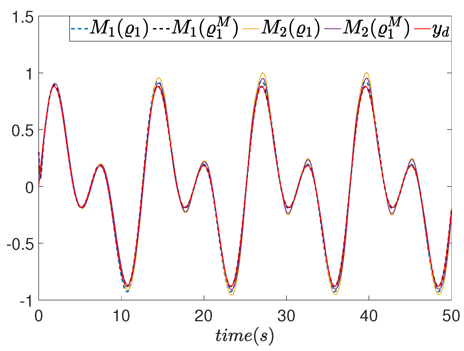
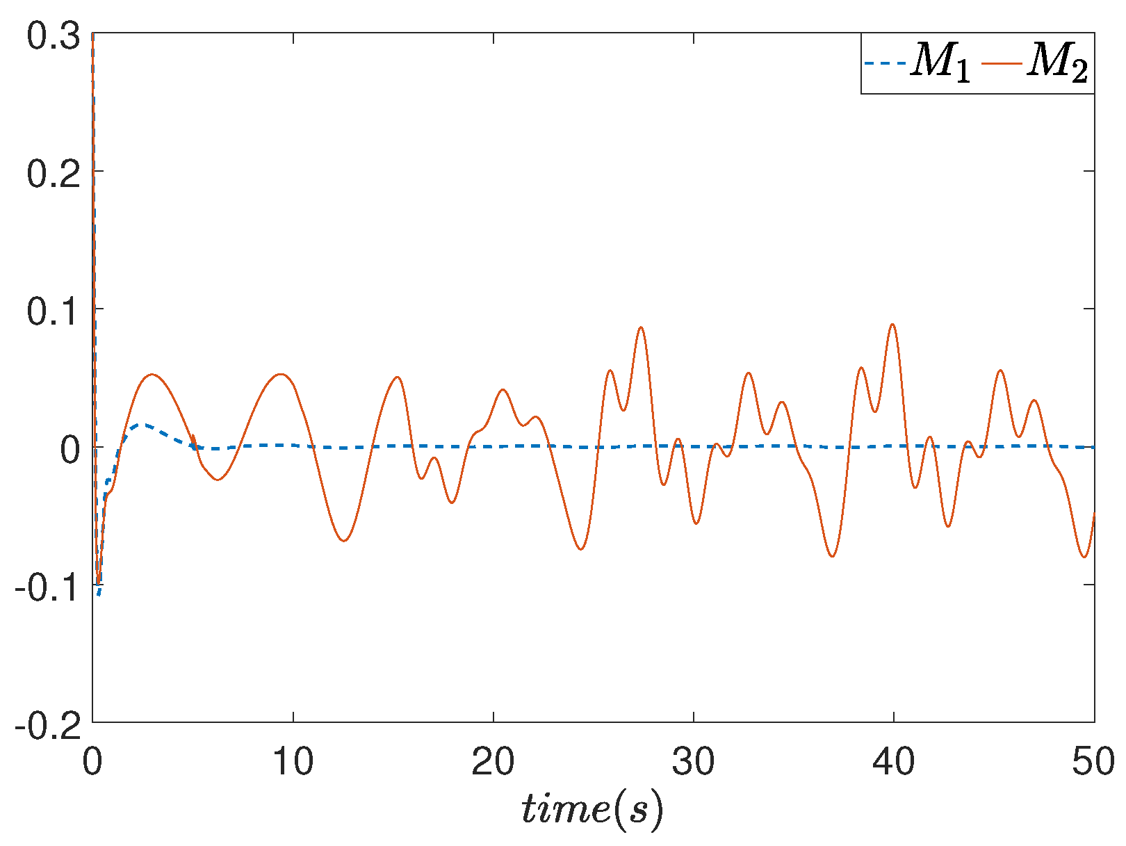
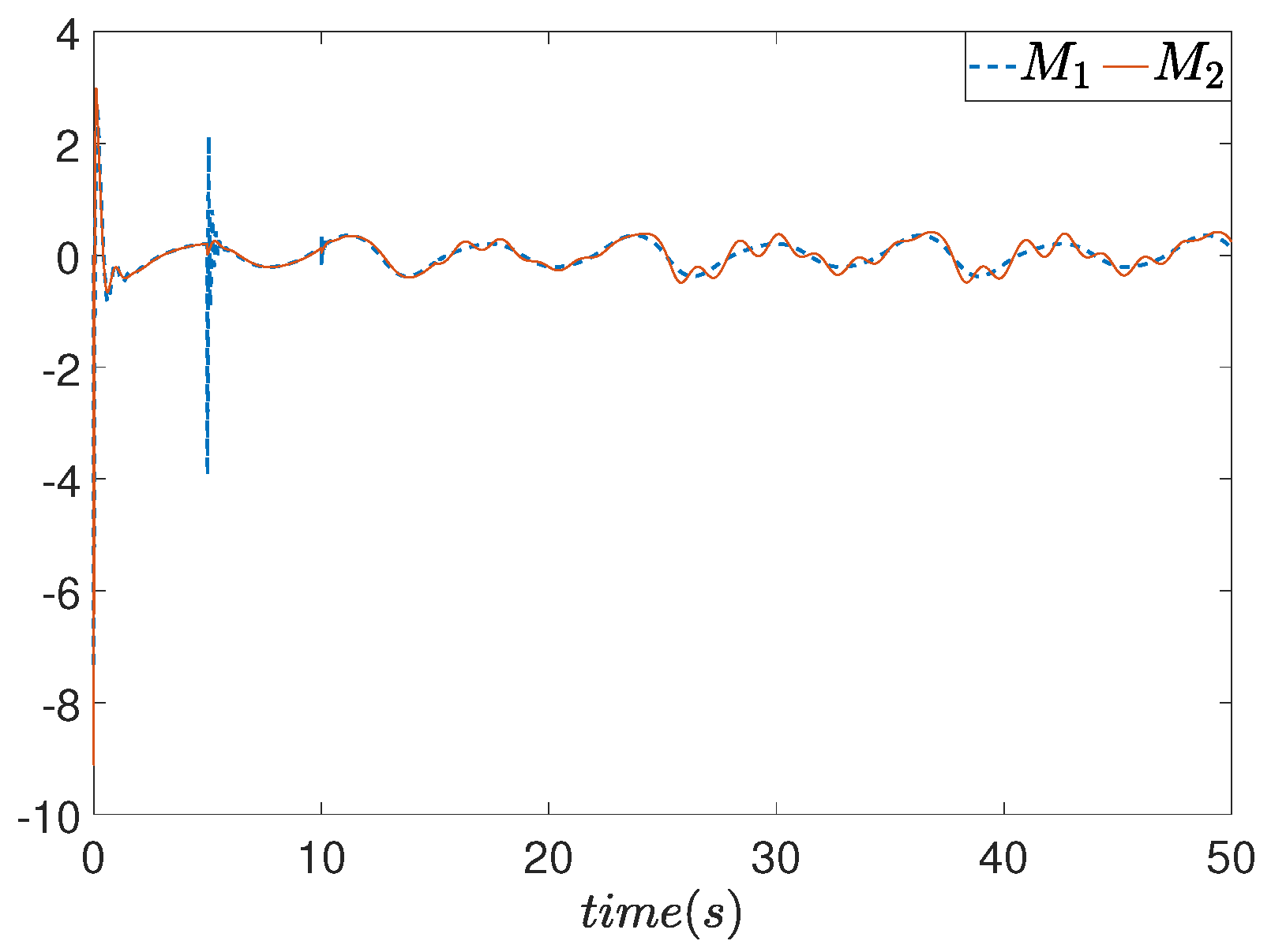
6. Simulation Results

To validate the effectiveness of this method, numerical simulations were conducted. Furthermore, to demonstrate that this method is related only to the error and is independent of the model, it was applied to a case study of a stable flying tailless flying-wing UAV.
Example 1. 
Numerical example.
Consider the nonlinear systems as mentioned in [28].
ϱ ˙ 1 = 0.3 ϱ 1 2 + ϱ 2 + sin ϱ 2 ϱ ˙ 2 = 0.2 ϱ 2 sin ϱ 1 2 + u + u 3 3 y = ϱ 1
where ϱ 1 and ϱ 2 are system states and y is the output of system. The targeted trajectory y d = 0.5 ( sin ( t ) + sin ( 0.5 t ) ) .
The sensor fault model is determined by
ϱ 1 M = ϱ 1 ,   0   s < t < 5   s 0.05 e 4 t + 0.95 ϱ 1 ,   5   s t ,   ϱ 2 M = ϱ 2 ,   0   s < t < 10   s 0.05 e 4 t + 0.95 ϱ 2 ,   10   s t
where μ 1 ( t ) = μ 2 ( t ) = 0.05 e 4 t + 0.95 , ς 1 = ς 2 = 0 .
The actuator fault parameters (3) are given as
γ = 1 ,   0   s < t < 15   s 0.8 e 0.2 t + 0.2 ,   15   s t ,   δ = 0 ,   0   s < t < 15   s cos 2 ϱ 1 ϱ 2 ,   15   s t
Obviously, f 1 ( ϱ 1 , ϱ 2 ) and f 2 ( ϱ ¯ 2 , u ) is non-differentiable, but Assumption 1 can still be satisfied and our method is still valid, u denotes the systems input and u a is the actual control input.
Set the initial values as [ ϱ 1 , ϱ 2 ] T = [ 0.3 , 0.1 ] T , select the control coefficient and performance functions as κ 1 = 5 , κ 2 = 5 , ϖ 1 = 0.99 e 5 t + 0.01 , ϖ 2 = 0.9 e 5 t + 0.1 . To prove the superiority of the proposed algorithm, a comparison between the proposed method in this article (correspond to M1) and the control method developed in reference [28] (correspond to M2) in which the tracking errors and the parameters of the controller are designed as z 1 = ϱ 1 M y d , z 2 = ϱ 2 M α 1 , k 1 = 5 , k 2 = 5 , a 1 = 2 , a 2 = 10 , β = 4 , ϖ = 0.1 , λ ( 0 ) = 0 , and set the same initial values as [ ϱ 1 , ϱ 2 ] T = [ 0.3 , 0.1 ] T . The results of the simulation are presented in Figure 1, Figure 2, Figure 3 and Figure 4.
The control law and adaptive law in reference [28] are shown as follows:
α 1 = k 1 + 3 4 z 1 z 1 3 2 a 1 2 λ ^ S 1 T Z 1 S 1 Z 1 u a = k 2 + 3 4 z 2 z 2 3 2 a 2 2 λ ^ S 2 T Z 2 S 2 Z 2 λ ^ ˙ = i = 1 2 β 2 a i 2 z i 6 S i T Z i S i Z i ϖ λ ^
As shown in Figure 1 and Figure 2, although the proposed control method, as well as the technique reported in [26], both render that the system output has a great performance on tracking the reference trajectory, our proposed method has a smaller tracking error. From Figure 3 and Figure 4, it can be observed that the two methods have almost the same control inputs, which further demonstrates the superiority of our method. Moreover, we can see that all the system signals are bounded.
Example 2. 
Practical example.
To verify the advantages of the developed methodology over existing approaches, practical simulations incorporating tailless flying-wing Unmanned Aerial Vehicles (UAVs) with sensor faults are introduced. Adhering to the Newton–Euler framework, the comprehensive six-degree-of-freedom (6-DoF) dynamics of the UAV are delineated as follows Figure 5:
p ˙ = R 1 φ v ,
v ˙ = S w v + F T m + R 1 T φ g + F a m + d v ( t ) ,
φ ˙ = R 2 φ w ,
J w ˙ = w × Jw + M a + C δ + Jd w ( t ) ,
where p = x , y , z T signify the coordinates within the inertial reference frame O x I y I z I , v = u , v , w T represent the linear velocity relative to the body-fixed frame O x b y b z b , φ = ϕ , θ , ψ T encapsulates the orientation via Euler angles, encompassing the roll angle, pitch angle and yaw angle, the angular velocity vector w = p , q , r T is also defined with respect to O x b y b z b . Furthermore, F T = T , 0 , 0 T symbolizes the thrust vector, while δ = [ δ 1 L , δ 2 L , δ 3 L , δ 4 L , δ 1 R , δ 2 R , δ 3 R , δ 4 R ] T is the control inputs. The UAV’s mass is denoted by m, and g = 0 , 0 , g T indicates the gravitational acceleration vector in O x I y I z I . The external disturbances affecting the translational and rotational dynamics are represented by d v t and d w t , respectively, which are assumed to be unknown but confined within certain limits. The cross-product matrix S w is defined subsequently. Lastly, the inertia tensor J is expressed in O x b y b z b (with the x z plane-symmetric):
S w = 0 r q r 0 p q p 0
J = J x 0 J x z 0 J y 0 J z x 0 J z
The aerodynamic forces, denoted by F a , and the aerodynamic torques, represented by M a are described as follows
F a = F x , F y , F z T = Q S w R 3 1 C D , C Y , C L T M a = l a , m a , n a T = Q S w b C l , c C m , b C n T
where c symbolize the average aerodynamic chord, and b represent the span of the wings. The dynamic pressure, denoted by Q, is given by 1 2 ρ V 2 , ρ , where r h o , and the total velocity V are determined by the expressions α = arctan ( w / u ) , β = arcsin ( v / V ) , and V = v = u 2 + v 2 + w 2 , respectively. The dimensionless coefficients C D , C Y , C L , C l , C m , C n are used to characterize aerodynamic forces and moments. Furthermore, the control effectiveness matrix C is defined as:
C = Q S w b C l δ a 0 Q S w b C l δ r 0 Q S w c C m δ e 0 Q S w b C n δ a 0 Q S w b C n δ r .
The matrix R 1 ( φ ) serves to convert coordinates from the body frame to the inertial frame, whereas R 2 ( φ ) translates the angular velocity in the non-inertial frame into its corresponding time derivative with respect to the Euler angles. Furthermore, R 3 ( α , β ) aligns the body frame coordinates with a virtual wind frame that is oriented according to the aircraft’s relative velocity vector. The mathematical expressions for these transformation matrices are delineated as follows:
R 1 = c ψ c θ s ψ c ϕ + c ψ s θ s ϕ s ψ s ϕ + c ψ s θ c ϕ s ψ c θ c ψ c ϕ + s ψ s θ s ϕ c ψ s ϕ + s ψ s θ c ϕ s θ c θ s ϕ c θ c ϕ
R 2 = 1 s ϕ t θ c ϕ t θ 0 c ϕ s ϕ 0 sphi / c θ cphi / c θ
R 3 = c α c β s β s α c β c α s β c β s α s β s α 0 c α
where s, c and t stand for sin, cos and tan functions, respectively. The structural parameters and the aerodynamic coefficients for the flying-wing UAVs are sourced from the works of Zhou et al. [32].
The fault parameters of the linear velocity and Euler Angle sensors are determined by
μ V = 1 0.5 sin ( t ) tanh ( t ) , ς V = 0.2 sin ( t ) μ φ = 1 0.2 tanh ( t ) , ς φ = 0.1 tanh ( t ) μ θ = 1 0.2 cos ( t ) tanh ( t ) , ς θ = 0.1 cos ( t ) μ ψ = 1 0.1 tanh ( t ) , ς ψ = 0.5 tanh ( t )
and the actuator faults parameters (3) are given as
γ T ( t ) = 0.9 ,   0 t < 10 1 ,   10 t ,   δ T ( t ) = 0.1 e t ,   0 t < 10 0 ,   10 t
The reference models, which satisfy realistic performance, have been selected as follows:
V ¨ r ( t ) + 1.8 V ˙ r ( t ) + V r ( t ) = V c ( t ) , Ω ¨ r ( t ) + 1.8 Ω ˙ r ( t ) + Ω r ( t ) = Ω c ( t )
the desired trajectories are presented by V r ( t ) and Ω r ( t ) , V c ( t ) and Ω c ( t ) are input signals, which are defined as
V c = 70 m / s ,   t = 0   s 90 m / s ,   0   s < t ,
Ω c = [ 0 deg , 2 deg , 0 deg ] T ,   t = 0   s [ 0 deg , 6 deg , 0 deg ] T ,   0   s < t 8   s [ 35 deg , 6 deg , 0 deg ] T ,   8   s < t 9   s [ 35 deg , 2 deg , 0 deg ] T ,   9   s < t 17   s [ 0 deg , 2 deg , 0 deg ] T ,   17   s < t
Select the UAV in the stable flight phase, and the initial states are chosen as p = [ 50 , 0 , 200 ] T , v = [ 70 , 0 , 0 ] T , Ω = [ 0 deg , 2 deg , 0 deg ] T , w = [ 0 deg / s , 0 deg / s , 0 deg / s ] T , d v = [ sin ( t ) , sin ( t ) , sin ( t ) ] T , d ω = sin ( t ) , sin ( t ) , sin ( t ) T . The control parameters and performance functions are selected as k V = 50 , k Ω = 100 , k w = 100 , k v = k Ω = k w = 0.9 e 2 t + 0.1 . To realize control for a tailless aircraft, the pseudo-inverse method is used for control allocation, then the speed controller T, the virtual control law Ω and the control law δ are designed as
T = k V h 1 tan ( e V ) w = k Ω R 3 ( Ω ) tan ( e Ω ) δ = k w C 0 T ( C 0 C 0 T ) 1 tan ( e Ω )
The control parameters and performance functions are selected as λ 1 = 5 , λ 2 = 5 , k 1 = 0.99 e 5 t + 0.01 , k 2 = 0.9 e 5 t + 0.1 . The simulation results are shown in Figure 6, Figure 7, Figure 8, Figure 9, Figure 10 and Figure 11. From Figure 6 and Figure 7, it is seen that the speed and Euler angles of the UAV under sensor faults and actuator faults can track the desired trajectory very well. From Figure 8, it can be seen that the tracking errors are very small. From Figure 9 and Figure 11, we can see that the actual control inputs are bounded. From the simulation of the tailless flying-wing UAV, we can further see that the proposed control method is only related to tracking errors.

7. Conclusions

A low-complexity global control method, irrespective of initial condition, is proposed to investigate the issue of tracking in pure-feedback systems with sensor faults and actuator faults in the case of non-differentiable non-affine functions. First, the non-affine functions are reconstructed by a novel modeling approach, and the requirement that non-affine function is differentiable is removed. Second, by introducing inverse-tangent functions to construct the transformation for tracking errors, a global controller ensures the system-prescribed performance is designed, which is only related to tracking errors. To certify the validity of this approach, the numerical simulation and simulation of tailless fly-wing UAVs are presented.

Author Contributions

Software, J.J.; Formal analysis, J.X.; Investigation, Y.C.; Resources, L.Y. and J.J.; Writing—original draft, C.H.; Writing—review & editing, C.H.; Supervision, Z.L. and Q.L.; Funding acquisition, Q.L. and Y.C. All authors have read and agreed to the published version of the manuscript.

Funding

This research was supported by the National Natural Science Foundation of China and the National Science Foundation of Shaanxi Province, China, grant numbers 62106284 and 2023-JC-YB-522.

Data Availability Statement

Data are contained within the article.

Conflicts of Interest

The authors declare no conflict of interest.

References

  1. Liu, Z.; Huang, H.; Park, J.; Huang, J.; Wang, X.; Lv, M. Adaptive fuzzy control for unknown nonlinear multiagent systems with switching directed communication topologies. IEEE Trans. Fuzzy Syst. 2023, 31, 2487–2494. [Google Scholar] [CrossRef]
  2. Liu, Z.; Huang, J.; Wen, C.; Su, X. Distributed control of nonlinear systems with unknown time-varying control coefficients: A novel Nussbaum function approach. IEEE Trans. Autom. Control 2023, 68, 4191–4203. [Google Scholar] [CrossRef]
  3. Meng, W.; Yang, Q.; Jagannathan, S.; Sun, Y. Distributed control of high-order nonlinear input constrained multiagent systems using a backstepping-free method. IEEE Trans. Cybern. 2019, 49, 3923–3933. [Google Scholar] [CrossRef] [PubMed]
  4. Boulkroune, A.; Haddad, M.; Li, H. Adaptive fuzzy control design for nonlinear systems with actuation and state constraints: An approach with no feasibility condition. ISA Trans. 2023, 142, 1–11. [Google Scholar] [CrossRef] [PubMed]
  5. Chen, L.; Wang, Q.; Hu, C. Adaptive fuzzy command filtered backstepping control for uncertain pure-feedback systems. ISA Trans. 2022, 129, 204–213. [Google Scholar] [CrossRef] [PubMed]
  6. Tao, F.; Fan, P.; Fu, Z.; Wang, N.; Wang, Y. Adaptive fuzzy fixed time control for pure-feedback stochastic nonlinear systems with full state constraints. J. Frankl. Inst. 2022, 359, 4642–4660. [Google Scholar] [CrossRef]
  7. Shi, W. Adaptive fuzzy output-feedback control for nonaffine MIMO nonlinear systems with prescribed performance. IEEE Trans. Fuzzy Syst. 2021, 29, 1107–1120. [Google Scholar] [CrossRef]
  8. Wang, N.; Fu, Z.; Song, S.; Wang, T. Barrier-lyapunov-based adaptive fuzzy finite-time tracking of pure-feedback nonlinear systems with constraints. IEEE Trans. Fuzzy Syst. 2022, 30, 1139–1148. [Google Scholar] [CrossRef]
  9. Wu, Z.; Zhang, T.; Xia, X.; Yi, Y. Finite-time adaptive neural command filtered control for pure-feedback time-varying constrained nonlinear systems with actuator faults. Neurocomputing 2022, 490, 193–205. [Google Scholar] [CrossRef]
  10. Wang, N.; Fu, Z.; Tao, F.; Song, S.; Wang, T. A simplified adaptive tracking control for nonlinear pure-feedback systems with input delay and full-state constraints. Int. J. Adapt. Control. Signal Process. 2021, 35, 2521–2536. [Google Scholar] [CrossRef]
  11. Wang, S. Asymptotic tracking control for nonaffine systems with disturbances. IEEE Trans. Circuits Syst.-Express Briefs 2022, 69, 479–483. [Google Scholar] [CrossRef]
  12. Wang, X.; Jiang, G.; Su, H.; Wang, X. Robust global coordination of networked systems with input saturation and external disturbances. IEEE Trans. Syst. Man-Cybern.-Syst. 2021, 51, 7788–7800. [Google Scholar] [CrossRef]
  13. Cheng, H.; Song, Y. Neuroadaptive tracking control for uncertain pure-feedback systems under dynamic constraints. Int. J. Robust Nonlinear Control 2023, 33, 6087–6102. [Google Scholar] [CrossRef]
  14. Niu, B.; Wang, X.; Wang, X.; Li, T. Adaptive barrier-lyapunov-functions based control scheme of nonlinear pure-feedback systems with full state constraints and asymptotic tracking performance. J. Syst. Sci. Complex. 2024, 37, 965–984. [Google Scholar] [CrossRef]
  15. Zhu, J.; Li, S. Adaptive output dynamic feedback control for nonaffine pure-feedback time delay system with unknown backlash-like. J. Frankl.-Inst.-Eng. Appl. Math. 2024, 361. [Google Scholar] [CrossRef]
  16. Zheng, A.; Huang, Y.; Na, J.; Shi, Q. Adaptive neural identification and non-singular control of pure-feedback nonlinear systems. ISA Trans. 2024, 144, 409–418. [Google Scholar] [CrossRef] [PubMed]
  17. Jia, J. Non-overshooting control of nonlinear pure-feedback systems. Syst. Control. Lett. 2024, 185, 105743. [Google Scholar] [CrossRef]
  18. Liu, Z.; Dong, X.; Xue, J.; Li, H.; Chen, Y. Adaptive neural control for a class of pure-feedback nonlinear systems via dynamic surface technique. IEEE Trans. Neural Netw. Learn. Syst. 2016, 27, 1969–1975. [Google Scholar] [CrossRef] [PubMed]
  19. Liu, Z.; Dong, X.; Xie, W.; Chen, Y.; Li, H. Adaptive fuzzy control for pure-feedback nonlinear systems with nonaffine functions being semibounded and indifferentiable. IEEE Trans. Fuzzy Syst. 2018, 26, 395–408. [Google Scholar] [CrossRef]
  20. Zuo, R.; Dong, X.; Chen, Y.; Liu, Z.; Shi, C. Adaptive neural control for a class of non-affine pure-feedback nonlinear systems. Int. J. Control 2019, 92, 1354–1366. [Google Scholar] [CrossRef]
  21. Zhai, D.; An, L.; Li, X.; Zhang, Q. Adaptive fault-tolerant control for nonlinear systems with multiple sensor faults and unknown control directions. IEEE Trans. Neural Netw. Learn. Syst. 2018, 29, 4436–4446. [Google Scholar] [CrossRef] [PubMed]
  22. Liu, X.; Zhai, D.; Dong, J.; Zhang, Q. Adaptive fault-tolerant control with prescribed performance for switched nonlinear pure-feedback systems. J. Frankl. Inst.-Eng. Appl. Math. 2018, 355, 273–290. [Google Scholar] [CrossRef]
  23. Ma, L.; Wang, Z.; Wang, C. Adaptive neural network state constrained fault-tolerant control for a class of pure-feedback systems with actuator faults. Neurocomputing 2022, 490, 431–440. [Google Scholar] [CrossRef]
  24. You, G.; Shen, Z.; Xu, B.; Zhang, C.; Zhao, S.; Hou, X.; Liu, Z. Adaptive fuzzy finite-time fault-tolerant control design for nonlinear pure-feedback systems with sensor faults. Int. J. Adapt. Control Signal Process. 2023, 37, 2000–2020. [Google Scholar] [CrossRef]
  25. Cao, L.; Li, H.; Dong, G.; Lu, R. Event-triggered control for multiagent systems with sensor faults and input saturation. IEEE Trans. Syst. Man Cybern.-Syst. 2021, 51, 3855–3866. [Google Scholar] [CrossRef]
  26. Liu, X.; Zhai, D.; Li, T.; Zhang, Q. Fuzzy-approximation adaptive fault-tolerant control for nonlinear pure-feedback systems with unknown control directions and sensor failures. Fuzzy Sets Syst. 2019, 356, 28–43. [Google Scholar] [CrossRef]
  27. Huang, X.; Wen, C.; Song, Y. Adaptive neural control for uncertain constrained pure feedback systems with severe sensor faults: A complexity reduced approach. Automatica 2023, 147, 110701. [Google Scholar] [CrossRef]
  28. Bali, A.; Chouhan, S.S.; Kumar, G.; Kumar, R.; Singh, U.P. Adaptive fault-tolerant control for pure-feedback stochastic nonlinear systems with sensor and actuator faults. Circuits Syst. Signal Process. 2023, 42, 5838–5867. [Google Scholar] [CrossRef]
  29. Jiang, Y.; Niu, B.; Zong, G.; Zhao, X.; Zhao, P. Distributed adaptive secure consensus tracking control for asynchronous switching nonlinear MASs under sensor attacks and actuator faults. IEEE Trans. Autom. Sci. Eng. 2023; early access. [Google Scholar] [CrossRef]
  30. Li, D.; Han, H.; Qiao, J.F. Fuzzy-Approximation Adaptive Fault Tolerant Control for Nonlinear Constraint Systems With Actuator and Sensor Faults. IEEE Trans. Fuzzy Syst. 2024, 32, 2614–2624. [Google Scholar] [CrossRef]
  31. Zhou, S.; Song, Y. Prescribed performance neuroadaptive fault-tolerant compensation for MIMO nonlinear systems under extreme actuator failures. IEEE Trans. Syst. Man Cybern. Syst. 2021, 51, 5427–5436. [Google Scholar] [CrossRef]
  32. Zhou, Y.; Dong, W.; Chen, Y.; Lv, M.; Zhang, B.; Xue, J. Distributed synchronization control for multiple tailless flying-wing UAVs with predefined tracking accuracy and input nonlinearities. Int. J. Robust Nonlinear Control 2023, 33, 3491–3516. [Google Scholar] [CrossRef]
Figure 1. Trajectories of ϱ 1 , ϱ 1 ( M ) and y d .
Electronics 13 03166 g001
Figure 2. Tracking error ϱ 1 ( M ) y d .
Electronics 13 03166 g002
Figure 3. The curves of u a .
Electronics 13 03166 g003
Figure 4. The curves of u.
Electronics 13 03166 g004
Figure 5. UAV coordinate system.
Electronics 13 03166 g005
Figure 6. Trajectories of V r and V m .
Electronics 13 03166 g006
Figure 7. The curves of φ r , φ m , θ r , θ m , ψ r , ψ m .
Electronics 13 03166 g007
Figure 8. The curves of tracking errors.
Electronics 13 03166 g008
Figure 9. The curve of T.
Electronics 13 03166 g009
Figure 10. The curves of δ L .
Electronics 13 03166 g010
Figure 11. The curves of δ R .
Electronics 13 03166 g011
Disclaimer/Publisher’s Note: The statements, opinions and data contained in all publications are solely those of the individual author(s) and contributor(s) and not of MDPI and/or the editor(s). MDPI and/or the editor(s) disclaim responsibility for any injury to people or property resulting from any ideas, methods, instructions or products referred to in the content.

