Abstract
The single-phase photovoltaic energy storage inverter represents a pivotal component within photovoltaic energy storage systems. Its operational dynamics are often intricate due to its inherent characteristics and the prevalent usage of nonlinear switching elements, leading to nonlinear characteristic bifurcation such as bifurcation and chaos. In this paper, a deep investigation of a single-phase H-bridge photovoltaic energy storage inverter under proportional–integral (PI) control is made, and a sinusoidal delayed feedback control (SDFC) strategy to mitigate the nonlinear characteristics is proposed. A frequency domain mapping model of the system is established, then, by analyzing the Jacobian matrix and equilibrium points, the bifurcation diagram is formed, and finally, the stable operational domains are determined under double and triple bifurcation parameters. Through simulation experiments, the efficacy of this strategy is validated. The findings show that through the control strategy, the stable operational envelope of the inverter can be greatly expanded and the nonlinear dynamic phenomena can be notably suppressed.
1. Introduction
Power electronic devices typically incorporate various switching components and nonlinear loads, exhibiting intricate nonlinear characteristics. The H-bridge inverter, a commonly used power electronics component, is widely applied in distributed generation, microgrids, energy storage systems, and various other power electronic systems. As a typical nonlinear system, the H-bridge inverter displays complex dynamic behaviors that significantly impact the stability and reliability of the system. Should the circuit parameters be improperly designed, the system may experience electromagnetic noise, intermittent oscillations, or even a sudden collapse during operation, posing a severe threat to the operational stability of the system [1,2,3]. This chaotic behavior in inverters can lead to severe output voltage and current distortions, significantly reducing the power quality conversion efficiency and inverter lifespan [4,5]. Due to its randomness, the system’s operational state becomes unpredictable, significantly impacting the control performance and potentially leading to complete failure. Omar et al. review various control methods in power systems and propose a novel optimized PID-based model reference fractional adaptive controller, but it has not been applied to a nonlinear system [6]. Therefore, finding an effective method to suppress the chaotic behavior of photovoltaic energy storage inverters is of great significance.
In light of this, developing a control method capable of effectively suppressing bifurcation and chaotic behaviors holds significant theoretical value and practical importance for enhancing the system stability and reliability. In recent years, numerous scholars and experts have conducted in-depth research into the nonlinear dynamic behaviors of H-bridge inverters to address the issues arising from their complex dynamics.
Robert et al. establish a discrete iterative model of a current-controlled H-bridge converter and conduct an in-depth analysis of the border collision bifurcation phenomenon [7,8]. Wang Xuemei et al. explore the bifurcation and chaotic phenomena in H-bridge inverters under proportional control [9]. Wang et al. analyze the fast-scale and slow-scale stability of the system using a discrete model of a single-phase full-bridge inverter, elucidating the interrelationship between these stability scales [10]. Tao et al. explore a dual-buck inverter’s stability and dynamic behavior under sliding mode control with an improved exponential approach law [11]. Bandyopadhyay et al. analyze the bifurcation phenomena in inverters with nonlinear rectifier loads using Filippov’s method and state-space averaging [12]. Wu et al. propose an improved discrete-time model for a digitally controlled single-phase full-bridge voltage inverter, predicting stability boundaries and oscillation frequencies [13]. Lei et al. show a unified “scalar” discrete-time model proposed for enhanced bifurcation prediction in a digitally controlled H-bridge grid-connected inverter system [14]. Dai Lu et al. investigate the nonlinear dynamic behaviors of a single-phase inverter under PI control [15]. Jiang Wei et al. examine the stability of an H-bridge inverter with PI control by applying fast-scale stability theory [16]. Ye Shi et al. establish state-space average and discrete-time models for three-phase full-bridge inverters employing sinusoidal pulse width modulation and space vector modulation, obtaining system stability boundaries [17]. The bifurcation and chaotic phenomena of three-phase grid-connected inverters under quasi-PR regulation are studied in [18], and their nonlinear behavior on fast timescales is analyzed. These studies indicate the presence of nonlinear behavior in the system but have not employed effective control methods to suppress chaotic phenomena. Robert et al. employ delayed feedback control to suppress nonlinear behavior in single-phase H-bridge inverters [19]. Zhou, L et al. indicate that washout filters mitigate the nonlinear dynamic behavior in single-phase H-bridge inverters [20].
This paper proposes a sine delayed feedback control (SDFC) method integrated with PI control principles to expand the stable operational range of single-phase H-bridge photovoltaic energy storage inverters. By addressing instability issues in critical operational scenarios, the power quality can be improved and the operational lifespan of the inverters can be extended, thereby improving the overall system reliability. Additionally, through the proposed method, the system’s robustness against disturbances can be increased, and stable operation under external perturbations is ensured. This robustness is critical for photovoltaic inverters, which must operate efficiently under various environmental conditions, including sunlight intensity and temperature variations, directly impacting the input voltage. The expanded stable region affords greater flexibility in system design and operation, enabling engineers to select from a broader range of , E, and L values to optimize performance without compromising stability. SDFC utilizes the difference between the inductor current and its delayed value over one period as feedback, which is processed through a sine function and multiplied by an adjustment coefficient before being applied to the control signal. A discrete mathematical model is established for the control scheme, and the system’s nonlinear dynamic behavior is observed through bifurcation diagrams and Jacobian matrices. The theoretical correctness is verified through simulation experiments. This method dramatically increases the stable operational range of the single-phase photovoltaic energy storage inverter, improves the system robustness, and establishes a dependable theoretical foundation for designing photovoltaic energy storage inverters.
The remaining article is organized as follows: Section 2 elaborates on the discrete mathematical modeling approach used for the photovoltaic energy storage inverters. Section 3 investigates the chaotic phenomena caused by PI control in photovoltaic energy storage inverters and examines their dynamic behaviors and stability challenges. Section 4 further explores the dynamic characteristics of inverters with EDFC introduced. Section 5 presents the SDFC strategy and systematically analyzes its superiority and potential applications in photovoltaic energy storage inverters. Section 6 validates the effectiveness and accuracy of the SDFC strategy through a simulation. Finally, Section 7 provides a summary of the entire study.
2. Operation Principle and System Model of the PI-Controlled Photovoltaic Energy Storage Inverter
The operation principle of the photovoltaic energy storage inverter with a PI controller is illustrated in Figure 1. The DC-side voltage of the inverter is supplied by a power source charged by the photovoltaic array through boost voltage.
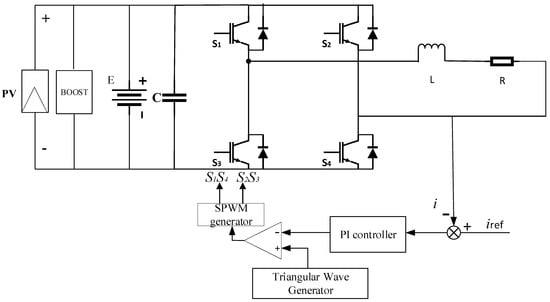
Figure 1.
Schematic diagram of photovoltaic energy storage inverter with PI regulator.
Figure 2 illustrates the specific process of controlling each switch transistor through SPWM modulation by the modulation signal . Based on the photovoltaic energy storage inverter controlled by PI, the circuit has two operation states within a switching cycle. The modulation signal undergoes comparison with the triangular wave . IH and IL, respectively, represent the maximum and minimum values of the triangular carrier waveform .
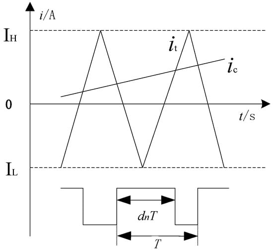
Figure 2.
Operation states of the inverter.
The first state: when is greater than , the PWM outputs a high level, S1 and S4 are turned on, and S2 and S3 are turned off. The second state: when is less than , the PWM outputs a low level, S1 and S4 are turned off, and S2 and S3 are turned on, as shown in Figure 1.
The duty cycle of state 1, denoted as , is expressed in Equation (1):
The inverter alternates between states 1 and 2, with the state equations for the main circuit during the nth switching cycle, T, provided by Equations (2) and (3).
In line with the frequency domain mapping theory, the selection of the switching period T serves as the time interval for frequency domain sampling. The sampled values of the state variables from the nth switching cycle serve to calculate the values for the (n + 1)th cycle, enabling the derivation of the discrete iteration model of the inverter’s main circuit [21].
represents the inductor current value at the sampling time.
The transfer function G(s) of the PI regulator and the relationship between the input and the output of the PI regulator can be obtained from the control circuit of the system:
denotes the discrepancy between the reference current and the current . This is combined with the previous Equation (5), as follows:
Let
The time-domain expression corresponding to Equation (6) is shown in Equation (8):
The reference current is discretized with the switching period T as the sampling period, assuming = . represents the maximum value of the reference signal. Considering the discrete derivation, given that fs >> f, the variable f represents the reference signal frequency, while fs denotes the system switching frequency. can be treated as a constant value, that is, , where n is the switching cycle index, and T is the switching period. Then, in Equation (7) can be discretized as
Substituting Equations (2) and (3) into Equation (8) yields
Thus, the relationship between the control signal at time and time , as well as between time and time , can be obtained, as follows:
By substituting Equation (4) into Equations (12) and (13), the discrete iteration model of the circuit can be obtained. The discrete model of the single-phase photovoltaic energy storage inverter controlled by PI control is given by Equation (14):
where
3. Nonlinear Dynamics of Inverter without Chaos Control
Single-phase photovoltaic energy storage H-bridge inverters are crucial components in electrical energy conversion systems, facing various challenges in practical applications. Among them, the proportional coefficient () is a critical parameter for the PI controller, directly affecting the inverter’s performance. Simultaneously, the fluctuations in input voltage (E) and variations in load inductance (L) are the significant factors leading to nonlinear dynamic behaviors in the inverter. This paper explores these challenges and proposes control strategies to address them, aiming to improve the efficiency and reliability of single-phase photovoltaic energy storage H-bridge inverters.
The circuit parameters are as follows:
When is used as the bifurcation parameter, E = 300 V and L = 10 mH; when E is used as the bifurcation parameter, = 0.9 and L = 10 mH; and when L is used as the bifurcation parameter, = 0.9 and E = 300 V. The other parameters remain as their default settings. For the parameters , E, and L within the specified ranges, Equations (4) and (5) are iterated multiple times, and the initial transient results are discarded to ensure the system enters a stable state. After stabilization, Equations (4) and (5) are set to continue iterating and the main circuit current I is recorded after each iteration. And then bifurcation diagrams are plotted with , E, and L as the x-axis and the main circuit current I as the y-axis, respectively. By analyzing these diagrams, the variation in the complexity and stability can be revealed in the system dynamics with the different , E, and L values, and profound insights into the system’s dynamical characteristics are revealed. The bifurcation diagram is shown in Figure 3.
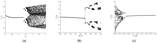
Figure 3.
Bifurcation diagrams in PI control mode with varying circuit parameters: (a) bifurcation diagram of the variation in inductor current with ; (b) bifurcation diagram of the variation in inductor current with ; (c) bifurcation diagram of the variation in inductor current with .
Figure 3a shows that under this control mode, for the stable boundary point at kp = 1.33, the system transitions from a stable state to an unstable chaotic state via a period-doubling bifurcation as kp increases from 0.1 to 3.0. The system operates stably between kp = 0.1 and kp = 1.33. In Figure 3b, a similar transition occurs as E increases from 200 V to 600 V, transitioning from a stable state to an unstable, chaotic state via a period-doubling bifurcation with a stable operating range from 200 V to 442 V. Additionally, Figure 3c illustrates that as L decreases from 20 mH to 2 mH, the system experiences a shift from a stable state to a period-doubling bifurcation and, ultimately, an unstable, chaotic state, and the system will remain stable with L between 20 mH and 7 mH. When kp is greater than 1.33, E will surpass 442 V, and when L decreases below 7 mH, the inverter system will enter a chaotic state. In this chaotic regime, the system experiences a deterioration in electrical power quality, alongside the increased thermal stress across the internal electronic components of the inverter. This results in a shortened inverter lifespan and reduced energy conversion efficiency.
By examining the eigenvalues of the Jacobian matrix, determined based on the system’s fixed points, the evaluation of the stability of a system can be made. If all the eigenvalues fall within the unit circle in the complex plane, the system is considered to be stable. However, if a pair of complex conjugate eigenvalues exit the unit circle as parameters change, the system undergoes a Hopf bifurcation. Similarly, if the eigenvalues cross the unit circle at −1, the system experiences a period-doubling bifurcation. By plotting the varying trajectories of these eigenvalues with the parameters, valuable insights into the system’s stability will be offered. This analytical approach allows researchers to understand how the parameter variations influence the system’s dynamics and predict its behaviors under different conditions.
Let x represent the system variables and μ denote the input or control parameter, then, to find the equilibrium points in a discrete system, the following differential equation can be established:
At the equilibrium points, the condition where the iterated value equals itself is satisfied, and can be expressed as the following equation:
From Equations (15)–(17), the equilibrium points , , and corresponding to the system output current , modulation signal , and duty cycle can be obtained.
Defining the state vector as yields
The Jacobian matrix at the equilibrium point can then be obtained as follows:
where .
The eigenvalues , and can be determined by solving the characteristic equation . Figure 4a–c illustrate the trajectories of the eigenvalues as kp varies from 0.1 to 3, E varies from 200 V to 600 V, and L varies from 1 mH to 20 mH. According to Figure 4a, when kp is 1.33, E is 442 V, and L is 7 mH, one of the eigenvalues intersects the unit circle while the other two remain inside the circle. Based on the stability criterion of the Jacobian matrix at the equilibrium point, it is inferred that a period-doubling bifurcation occurs at this point. As kp and E increase and L decreases, the eigenvalues begin to appear outside the unit circle in the complex plane, and the system progressively transitions towards instability, consistent with the results shown in Figure 3.
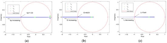
Figure 4.
Trajectories of system eigenvalue variation with circuit parameters: (a) trajectories of the variation in the system’s eigenvalues with from 0.1 to 3; (b) trajectories of the variation in the system’s eigenvalues with E from 200 V to 600 V; (c) trajectories of the variation in the system’s eigenvalues with from 1 mH to 20 mH.
4. Nonlinear Dynamics of Inverter with EDFC Chaos Control
Exponential Delay Feedback Control (EDFC) utilizes the difference between the system output and parameters delayed by a specific time, fed back to the chaotic system in the exponential form. Through this feedback, the operational state of the system is altered, enabling the system to transition from a chaotic state to stable single-cycle states [22,23]. In this study, the system switching period T is selected as the delay time.
Based on Figure 5 and the mechanism of EDFC, the discrete model of the modulation signal at this time is determined as
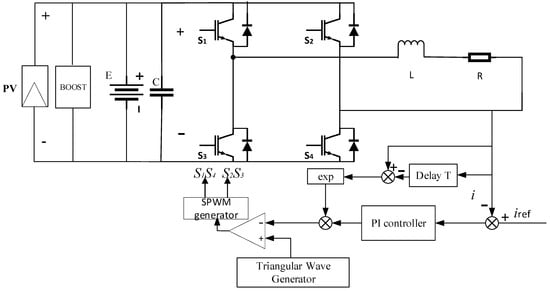
Figure 5.
Schematic diagram of photovoltaic energy storage inverter with an EDFC PI regulator.
At this time, the equilibrium point of the system remains unchanged, and the state variable of the system can be denoted as , and the Jacobian matrix of the system at this point can be calculated using Equation (21), as follows:
The three eigenvalues and of J2 can be obtained by solving the characteristic equation , and the trajectories of the variation in these eigenvalues with the parameters can be plotted.
Figure 6a–c illustrate the trajectories of the eigenvalues as kp varies from 0.1 to 2, E varies from 200 V to 600 V, and L varies from 1 mH to 20 mH. From Figure 6a, it can be seen that when kp is 1.58, E is 526 V, and L is 4.9 mH, one of the eigenvalues intersects the unit circle while the other two are still inside the circle. Based on the stability criterion of the Jacobian matrix at the equilibrium point, it is inferred that a period-doubling bifurcation occurs at this point. As kp and E increase and L decreases, the system progressively transitions towards instability. Moreover, when kp is reduced to 0.2, the pair of complex conjugate eigenvalues and cross the unit circle as kp decreases, indicating that the system undergoes a Hopf bifurcation, and when kp is between 0.2 and 1.58, E ranges from 200 V to 526 V, and L ranges from 20 mH to 4.9 mH, the system is still stable, outperforming the traditional PI control. But the addition of EDFC leads to a deterioration in the system’s stability when the proportional coefficient kp is small. This instability becomes more evident under certain conditions.
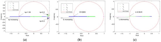
Figure 6.
Trajectories of system eigenvalue variation with circuit parameters: (a) trajectories of the variation in the system’s eigenvalues with from 0.1 to 2; (b) trajectories of the variation in the system’s eigenvalues with E from 200 V to 600 V; (c) trajectories of the variation in the system’s eigenvalues with from 1 mH to 20 mH.
Figure 6 shows that EDFC can effectively control the system when the bifurcation parameters deviate slightly from their stable values. However, when the bifurcation parameters deviate significantly, there is an issue of excessive disturbance caused by the feedback loop. Additionally, this control method lacks the ability to adjust the feedback intensity, thus making it difficult to achieve optimal control.
5. Nonlinear Dynamics of Inverter with SDFC Chaos Control
In response to the shortcomings mentioned above of applying EDFC to the PI control of single-phase energy storage H-bridge inverters for chaos control, a sinusoidal delay feedback control (SDFC) method is proposed. This method is mainly based on the improvement on EDFC, by which the chaos control effectiveness of photovoltaic energy storage H-bridge inverters can be effectively improved. Its basic principle can be described as follows: firstly, the difference between the controlled object’s output and its delayed value by one period is utilized as feedback, then, this feedback is multiplied by an adjustment coefficient , and then the result is passed through a sine function module; afterwards, the result is subtracted from 1 and multiplied by an adjustment coefficient , and finally, the final result is further multiplied by the original control signal. The system’s main and control circuits are depicted in Figure 7.
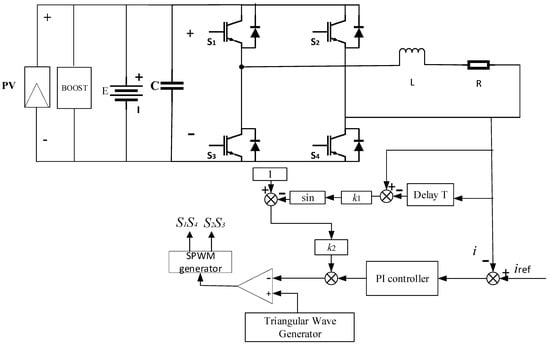
Figure 7.
Schematic diagram of photovoltaic energy storage inverter with SDFC PI regulator.
SDFC addresses the instability caused by excessive disturbance in the feedback loop by incorporating a sine function module and adjusting the feedback intensity through the adjustment coefficients and . This enhancement results in improved control effectiveness for the system.
Moreover, based on Figure 7 and the mechanism of SDFC, the discrete model of the modulation signal at this time is determined as
With the equilibrium point of the system remaining unchanged, and with the system’s state variable denoted as , the Jacobian matrix of the system at this point can be calculated using Equation (21), as follows:
The three eigenvalues and of J3 can be obtained by solving the characteristic equation , of which the characteristic polynomial is
where the coefficients are, respectively given by Equations (28) and (29),
To stabilize the system, all the characteristic roots must lie within the unit circle in the complex plane. The system’s stability determined by eigenvalues can be equivalently represented by According to the Jury stability criterion,
The values = 0.1 and = 0.2 can be selected. With the other parameters held constant, the bifurcation diagram is generated by combining Equations (4) and (25), where kp varies from 0.1 to 5, E ranges from 200 V to 1600 V, and L varies from 1 mH to 20 mH.
From the bifurcation diagram in Figure 8, it can be observed that the system remains stable when the proportional coefficient is increased to 3.89. The system also remains stable when the equivalent electromotive force of the power source is increased to 1245 V and the inductance is reduced to 2.7 mH.
Figure 8.
Bifurcation diagrams in SDFC mode with varying circuit parameters: (a) bifurcation diagram of the variation in inductor current with ; (b) bifurcation diagram of the variation in inductor current with ; (c) bifurcation diagram of the variation in inductor current with .
From Table 1, it can be observed that the introduction of SDFC significantly expands the parameter ranges for the stable operation of the system.

Table 1.
Parameter ranges (kp, E, L) for system stability under different control methods.
Figure 9 shows the trajectories of the variation in the system’s eigenvalues with parameters kp, E and L.
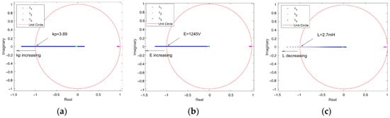
Figure 9.
Trajectories of system eigenvalue variation with circuit parameters: (a) trajectories of the variation in the system’s eigenvalues with from 0.1 to 5; (b) trajectories of the variation in the system’s eigenvalues with E from 200 V to 1600 V; (c) trajectories of the variation in the system’s eigenvalues with from 2 mH to 20 mH.
From the figure, it can be seen that when = 3.89, E = 1245 V, and L = 2.7 mH, the eigenvalue intersects the unit circle at −1, while and are in the unit circle. Based on the stability criterion of the Jacobian matrix at the equilibrium point, it can be inferred that the system undergoes a period-doubling bifurcation at this point. As kp and E increase and L decreases, the system gradually transitions to an unstable state. This observation is consistent with the results depicted in the bifurcation diagram in Figure 8.
Determining the instability boundary is crucial for system design purposes. Doing so assists engineers in selecting appropriate parameters during practical engineering tasks, thus avoiding the system from entering chaotic regions. Figure 10 illustrates the two-dimensional stability boundary formed by using the energy storage battery equivalent electromotive force E and the proportional coefficient as bifurcation parameters, the equivalent electromotive force E and the inductance L as bifurcation parameters, and the inductance L and the proportional coefficient as bifurcation parameters, with the other parameters of the system being constant. The stable operating region of the system is identified in the figure. Additionally, from Figure 10, it can be seen that the stable operating region obtained by the SDFC method is greater than that obtained by the EDFC and conventional PI control methods.
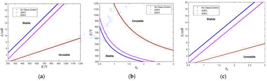
Figure 10.
Stability boundary: (a) stability boundary for the E and L parameters; (b) stability boundary for the and E parameters; (c) stability boundary for the and L parameters.
In conclusion, the stability of the photovoltaic energy storage inverter system is significantly influenced by the proportional coefficient , the equivalent electromotive force of the battery E, and the inductive load L. Therefore, the stable operating regions of the system under the traditional PI regulation and the enhanced SDFC regulation are presented with , E, and L as the bifurcation parameters. As shown in Figure 11, the region below the surface represents the stable operating domain, while the area above the surface indicates the system instability. It is evident that the incorporation of SDFC significantly expands the stable operating region.
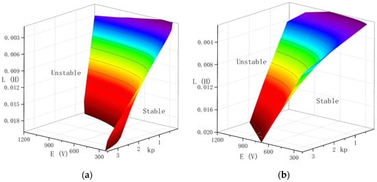
Figure 11.
Stability boundary: (a) stability boundary of PI control; (b) stability boundary of PI control with SDFC.
Figure 11a shows the stability boundary for the traditional PI control method. The stable region is relatively limited, indicating that the system is prone to instability with variations in the control parameter or the input voltage E. This constrained stability range poses a significant challenge for maintaining reliable inverter operation, particularly under the dynamic conditions as encountered in photovoltaic systems. Conversely, Figure 11b presents the stability boundary when SDFC is integrated with PI control. The plot demonstrates that the inclusion of SDFC substantially expands the stable operating region. This expanded stability range is crucial for photovoltaic energy storage inverters. The inclusion of SDFC significantly enhances the inverter system’s stability, making it more resilient to fluctuations in the control parameter and input voltage. This improvement is essential for ensuring continuous and reliable energy conversion and storage in photovoltaic applications, where maintaining stability under varying conditions is critical. The broader stability range underscores the robustness of the SDFC method. This robustness is vital for photovoltaic inverters, which must operate effectively under diverse environmental conditions, such as variations in sunlight intensity and temperature, and will directly affect the input voltage. The expanded stable region provides greater flexibility in system design and operation. Engineers can select from a wider range of and E values to optimize the performance without compromising stability. This flexibility is particularly beneficial for adapting the inverter to different photovoltaic panel configurations and storage requirements. By integrating SDFC, the photovoltaic energy storage inverter can achieve faster and more reliable stabilization of the output currents and voltages, even under sudden disturbances. This leads to a higher quality power output, reduced stress across electrical components, and extended equipment lifespan.
Additionally, the enhanced disturbance rejection capability ensures that the inverter can maintain stable operation in complex and dynamic photovoltaic environments, thus improving the overall efficiency and reliability of the energy storage system. In summary, incorporating SDFC into the control strategy of a photovoltaic energy storage inverter significantly enhances its stability, robustness, and flexibility. This improvement ensures the reliable operation under varying conditions and supports the improved performance and longevity of the inverter system, making SDFC a valuable control method for modern photovoltaic applications.
6. Simulation Verification
All simulations conducted to validate the findings were performed using MATLAB 2022b. To validate the numerical findings, simulations were conducted on a PI-controlled energy storage H-bridge inverter without chaos control. The parameters were set as follows: E = 300 V, = 0.9, ki = 150, R = 15 Ω, L = 10 mH, fs = 20 kHz, = 5 A, and f = 50 Hz. The simulations were conducted by individually changing one parameter, and the results are shown in Figure 12.
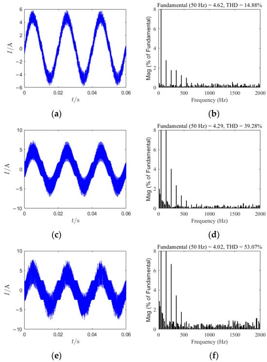
Figure 12.
Time-domain waveforms and total harmonic distortion without chaos control under various parameters: (a) the time-domain waveform diagram for = 3.5 without chaos control; (b) total harmonic distortion at = 3.5 without chaos control; (c) the time-domain waveform diagram for E = 800 V without chaos control; (d) total harmonic distortion at E = 800 V without chaos control; (e) the time-domain waveform diagram for L = 5 mH without chaos control; (f) total harmonic distortion at L = 5 mH without chaos control.
Figure 12a,b depict the time-domain waveform of the system’s output current and the total harmonic distortion (THD) under the condition where = 3.5 without chaotic control. The system exhibits a high level of harmonic content, with a THD as high as 14.88%. Similarly, in Figure 12c,d, the time-domain waveform of the system output current and THD are shown under the condition where E = 800 V without chaotic control, resulting in a high THD of 39.28%. Figure 12e,f illustrate the time-domain waveform of the system output current and THD under the condition where L = 5 mH without chaotic control, again with a high THD of 53.07%. Such excessive THD will cause significant disturbances to the system, rendering it unable to meet the requirements of the power system.
In Figure 13 is given the time-domain waveform of the system output current and the total harmonic distortion (THD) under the condition where = 3.5 under chaos control. At 0.06 s, the simulation starts, and EDFC and SDFC are introduced into the circuit, with the remaining parameters remaining unchanged. Figure 13a,b present the time-domain waveform and THD of the output current under EDFC when = 3.5. In this scenario, the output current exhibits a high level of harmonic content, with a total harmonic distortion coefficient of 14.90%. Conversely, Figure 13c,d illustrate the time-domain waveform and THD of the output current under SDFC with = 3.5. Under this condition, the total harmonic distortion coefficient decreases to 1.86% due to the reduced harmonic content in the output current. Under the same conditions, the decrease in the THD from 14.9% to 1.86% demonstrates the effectiveness of the SDFC strategy.
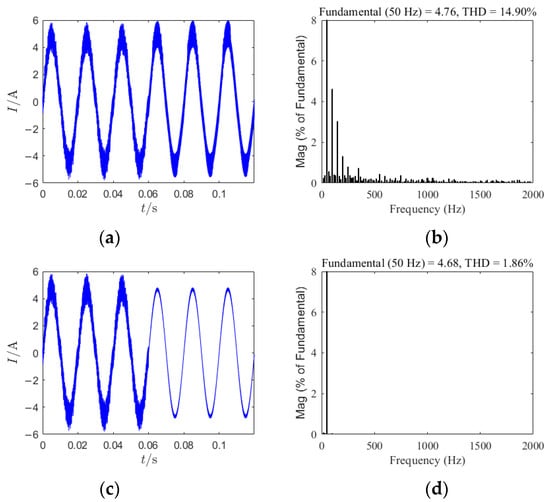
Figure 13.
Time-domain waveforms and total harmonic distortion: (a) the time-domain waveform diagram for = 3.5 under EDFC; (b) total harmonic distortion at = 3.5 under EDFC; (c) the time-domain waveform diagram for = 3.5 under SDFC; (d) total harmonic distortion at = 3.5 under SDFC.
In Figure 14 is given the time-domain waveform of the system output current and the total harmonic distortion (THD) under the condition where = 3.5 under chaos control. At 0.06 s, the simulation starts, and the EDFC and SDFC methods are introduced into the circuit, while the remaining parameters remain unchanged, with the inductance set at L = 3 mH. Figure 14a,b present the time-domain waveform and total harmonic distortion (THD) of the output current under EDFC. In this scenario, the output current exhibits a high level of harmonic content, with a THD of 60.79%. Conversely, Figure 14c,d illustrate the time-domain waveform and THD of the output current under SDFC. Under this condition, the harmonic content in the output current is significantly decreased, and the THD of which is reduced to 6.21%.
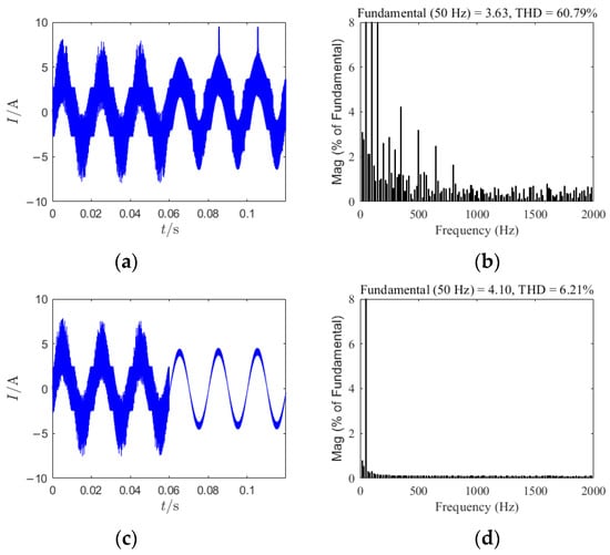
Figure 14.
Time-domain waveforms and total harmonic distortion: (a) the time-domain waveform diagram for L = 5 mH under EDFC; (b) total harmonic distortion at L = 5 mH under EDFC; (c) the time-domain waveform diagram for L = 5 mH under SDFC; (d) total harmonic distortion at L = 5 mH under SDFC.
In Figure 15 is given the time-domain waveform of the system output current and the total harmonic distortion (THD) under chaos control. At 0.06 s, the simulation starts, EDFC and SDFC are introduced into the circuit, and the remaining parameters remain unchanged. Figure 15a,b present the time-domain waveform and THD of the output current under EDFC when E = 800 V. In this scenario, the output current exhibits a high THD value, with a total harmonic distortion coefficient of 44.79%. Conversely, Figure 15c,d illustrate the time-domain waveform and THD of the output current under SDFC with E = 1200 V. Under this condition, the harmonic content in the output current is reduced, thus reducing the total harmonic distortion coefficient to 4.78%. Despite the significantly higher DC-side voltage in the SDFC method compared to the EDFC method, the THD under SDFC is markedly lower than that under EDFC. This demonstrates the substantial superiority of SDFC in harmonic suppression.
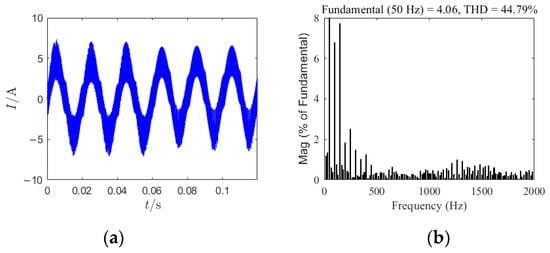
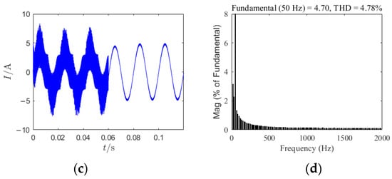
Figure 15.
Time-domain waveforms and total harmonic distortion: (a) the time-domain waveform diagram for E = 800 V under EDFC; (b) total harmonic distortion at E = 800 V under EDFC; (c) the time-domain waveform diagram for E = 1200 V under SDFC; (d) total harmonic distortion at E = 1200 V under SDFC.
Compared to the original PI control method, introducing EDFC leads to excessive disturbances, an increase in the inductance current THD, and a deterioration in the control performance when the system significantly deviates from the stable region, further exacerbating chaotic phenomena. Conversely, with the adoption of SDFC, the system transitions from an unstable state to a stable operation, resulting in a significant reduction in the inductance current THD and effectively suppressing chaotic behavior, thereby demonstrating outstanding control effectiveness.
In Figure 16 is given the comparison of the time-domain waveforms of the system output current under time-delay feedback control [7], filter-based chaos control [24], EDFC chaos control, EDFC with = 1.2 and E = 400 V, and with the other parameters unchanged. At 0.04 s, a disturbance of 100 V is applied to the DC-side of the system. Figure 16a–d depict the resulting AC-side current waveforms after applying these four chaos control methods. It can be observed that all the methods successfully transition the system from a chaotic state to a stable state; notably, the SDFC method exhibits the fastest response speed. Following the disturbance to the DC-side voltage, the time-delay feedback control, filter-based chaos control, and EDFC chaos control methods exhibit poorer disturbance rejection capabilities compared to the SDFC method, which maintains the stable operation of the system. The SDFC system shows significant response speed, disturbance rejection, and electrical energy quality advantages. The control method can respond to the variation in the system parameters and external disturbances rapidly, and minimize the system oscillations and instability duration effectively. Additionally, SDFC can also effectively suppress the oscillations and fluctuations during the regulation, ensuring a stable output current and voltage, thereby improving the electrical power quality. This high-quality electrical energy output reduces electrical and thermal stresses across the load equipment, prolonging the equipment lifespan and reducing the maintenance and replacement costs.
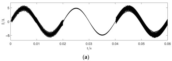
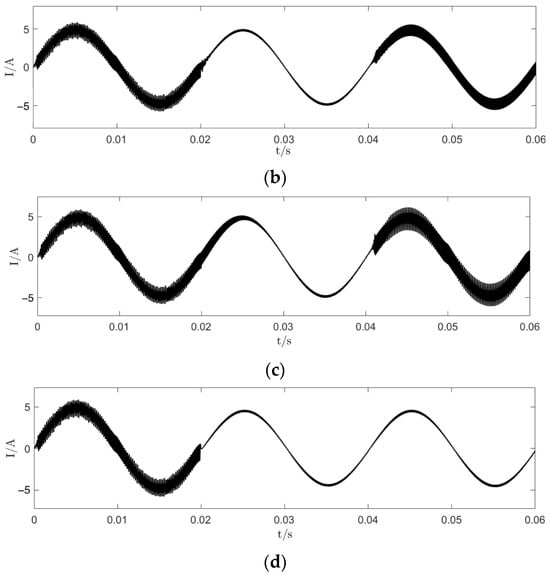
Figure 16.
Time-domain waveform diagram: (a) the time-domain waveform diagram under time-delay feedback control; (b) the time-domain waveform diagram under filter-based chaos control; (c) the time-domain waveform diagram under EDFC; (d) the time-domain waveform diagram under SDFC.
In response to the system disturbances, the SDFC system exhibits strong robust stability compared to the other methods, which display noticeable instability characteristics. This underscores the SDFC system’s capability to maintain stability in complex and dynamic operational environments, effectively reducing energy losses and improving the overall inverter efficiency and reliability.
This highlights the considerable advantage of the SDFC strategy in addressing the system deviations from the steady state and reducing chaotic phenomena, providing a viable solution for system stability and control performance.
7. Conclusions
From the perspective of nonlinear dynamics, this paper investigates a single-phase photovoltaic energy storage inverter under PI regulation, and a sinusoidal delayed feedback control method is proposed, detailing its fundamental principles. By establishing a discrete iterative model of the system, this study thoroughly explores the range of values for the control coefficient , the equivalent DC-side voltage E, and the inverter-side inductance L under stable operation. Additionally, based on the eigenvalues of the system’s Jacobian matrix, the stable operating regions under both the double-bifurcation and triple-bifurcation parameters are determined. Simulation experiments are conducted and compared with exponential delayed feedback control to validate this method’s effectiveness. The results indicate that using the proposed sinusoidal delayed feedback control method can effectively suppress the chaotic phenomena within the system and significantly expand the stable operating region. Compared to the other chaos controls, this approach demonstrates superior control performance with a faster response speed and better robustness in mitigating disturbances. By incorporating SDFC, the photovoltaic energy storage inverter achieves the swift stabilization of its outputs, and ensures high-quality power delivery. In addition, through this method, the strain of the components can be reduced, and the equipment lifespan can be extended. Moreover, the enhanced disturbance rejection enables its stable operation under dynamic conditions, thus boosting the system efficiency and reliability. These research findings provide the crucial theoretical underpinnings for designing and manufacturing photovoltaic energy storage inverters.
In future research, we plan to extend the application of the proposed SDFC strategy to cascaded and three-phase inverters. Additionally, efforts will focus on integrating grid synchronization capabilities.
Author Contributions
Conceptualization, T.L. and R.G.; methodology, T.L.; validation, T.L., Z.W. and Y.Q.; writing—original draft preparation, T.L.; writing—review and editing, T.L., R.G. and J.X.; project administration, R.G.; funding acquisition, R.G. All authors have read and agreed to the published version of the manuscript.
Funding
This research was funded by the National Natural Science Foundation of China, grant number 61561007, and the Natural Science Foundation of Guangxi Province, China, grant number 2017GXNSFAA198168.
Data Availability Statement
The data used to support the findings of the study are available within the article.
Conflicts of Interest
The authors declare no conflicts of interest.
References
- Alfayyoumi, M.; Nayfeh, A.; Borojevic, D. Modeling and Analysis of Switching-Mode DC-DC Regulators. Int. J. Bifurc. Chaos 2000, 10, 373–390. [Google Scholar] [CrossRef]
- Yu, Y.; Zhang, C. Bifurcation Analysis of Cascaded H-Bridge Converter Controlled by Proportional Resonant. Int. J. Electr. Power Energy Syst. 2021, 125, 106476. [Google Scholar] [CrossRef]
- Komurcugil, H.; Biricik, S.; Bayhan, S.; Zhang, Z. Sliding Mode Control: Overview of Its Applications in Power Converters. IEEE Ind. Electron. Mag. 2021, 15, 40–49. [Google Scholar] [CrossRef]
- Zhang, B. Study of Nonlinear Chaotic Phenomena of Power Converters and Their Applications. Trans. China Electrotech. Soc. 2005, 20, 12. [Google Scholar] [CrossRef]
- Yang, L.; Yang, L.; Yang, F.; Ma, X. Slow-Scale and Fast-Scale Instabilities in Parallel-Connected Single-Phase H-Bridge Inverters: A Design-Oriented Study. Int. J. Bifurc. Chaos 2020, 30, 2050005. [Google Scholar] [CrossRef]
- Omar, O.; Marei, M.; Attia, M. Comparative Study of AVR Control Systems Considering a Novel Optimized PID-Based Model Reference Fractional Adaptive Controller. Energies 2023, 16, 830. [Google Scholar] [CrossRef]
- Robert, B.; Robert, C. Border Collision Bifurcations in a One-Dimensional Piecewise Smooth Map for a PWNT Current-Programmed H-Bridge Inverter. Int. J. Control. 2002, 75, 1356–1367. [Google Scholar] [CrossRef]
- Iu, H.; Robert, B. Control of Chaos in a PWM Current-Mode H-Bridge Inverter Using Time-Delayed Feedback. IEEE Trans. Circuits Syst. i-Fundam. Theory Appl. 2003, 50, 1125–1129. [Google Scholar] [CrossRef]
- Wang, X.; Zhang, B. Study of Bifurcation and Chaos in Single-Phase SPWM Inverter. Trans. China Electrotech. Soc. 2009, 24, 101–107. [Google Scholar]
- Wang, X.; Zhang, B.; Qiu, D. The Fast- and Slow-Scale Stabilities and Chaotic Motion of H-Bridge Sine Inverter. Acta Phys. Sin. 2009, 58, 2248–2254. [Google Scholar] [CrossRef]
- Tao, H.; Ai, P. Dynamics Characteristics of Dual-Buck Inverter Under Improved Sliding Mode Control. Proc. CSU-EPSA 2023, 35, 130–136+144. [Google Scholar] [CrossRef]
- Bandyopadhyay, A.; Mandal, K.; Parui, S. A Filippov Method Based Analytical Perspective on Stability Analysis of a DC-AC H-Bridge Inverter with Nonlinear Rectifier Load. Int. J. Circuit Theory Appl. 2022, 50, 1686–1708. [Google Scholar] [CrossRef]
- Wu, X.; Xiao, G.; Lei, B. Improved Discrete-Time Model for a Digital Controlled Single-Phase Full-Bridge Voltage Inverter. Acta Phys. Sin. 2013, 62, 050503. [Google Scholar] [CrossRef]
- Lei, B.; Xiao, G.; Wu, X.; Zheng, L. A unified “scalar” discrete-time model for enhancing bifurcation prediction in digitally controlled h-bridge grid-connected inverter. Int. J. Bifurc. Chaos 2013, 23, 1350126. [Google Scholar] [CrossRef]
- Dai, L.; Long, Y. Study of Bifurcation and Chaos for Photovoltaic Inverter with PI Controller. Power Syst. Prot. Control 2012, 40, 89–94. [Google Scholar]
- Jiang, W.; Wu, R. A Study on Work_ing Stability of H-Bridge Inverter Based on PI Control. J. Vib. Shock. 2020, 39, 62–68. [Google Scholar]
- Shi, Y.; Wu, Z. Research on Bifurcation Behaviors of Three-Phase Full Bridge Inverters. Proc. CSEE 2016, 36, 19. [Google Scholar] [CrossRef]
- Tao, X.; Chen, Q.; Tian, L. Bifurcation analysis of Three-Phase Grid-Connected Inverters Based Onquasi PR Controller. Power Syst. Prot. Control. 2018, 46, 100–107. [Google Scholar]
- Robert, B.; Iu, H.; Feki, M. Adaptive Time-Delayed Feedback for Chaos Control in a PWM Single Phase Inverter. J. Circuits Syst. Comput. 2004, 13, 519–534. [Google Scholar] [CrossRef]
- Zhou, L.; Long, Y.; Xie, J. Controlling Chaos in H-Bridge Converter with Washout Filter. Power System Prot. Control 2013, 41, 32–37. [Google Scholar]
- Zhou, L.; Long, Y.; Guo, K.; Li, H.; Du, J. Bifurcation and Chaos of Inverter System Based on Coefficient Linear Model. Electr. Power Autom. Equip. 2013, 33, 100–104. [Google Scholar]
- Nakajima, H.; Ueda, Y. Limitation of Generalized Delayed Feedback Control. Physica D 1998, 111, 143–150. [Google Scholar] [CrossRef]
- Liu, X.; Huang, W. Delayed feedback control of chaotic systems and its theoretical and experimental researches. Adv. Mech. 2001, 31, 18–32. [Google Scholar]
- Lu, W.; Zhao, N.; Wu, J.; El Aroudi, A.; Zhou, L. Filter-Based Perturbation Control of Low-Frequency Oscillation in Voltage-Mode H-Bridge DC-AC Inverter. Int. J. Circuit Theory Appl. 2015, 43, 866–874. [Google Scholar] [CrossRef]
Disclaimer/Publisher’s Note: The statements, opinions and data contained in all publications are solely those of the individual author(s) and contributor(s) and not of MDPI and/or the editor(s). MDPI and/or the editor(s) disclaim responsibility for any injury to people or property resulting from any ideas, methods, instructions or products referred to in the content. |
© 2024 by the authors. Licensee MDPI, Basel, Switzerland. This article is an open access article distributed under the terms and conditions of the Creative Commons Attribution (CC BY) license (https://creativecommons.org/licenses/by/4.0/).