Beam Prediction for mmWave V2I Communication Using ML-Based Multiclass Classification Algorithms

Abstract

Beam management is a key functionality in establishing and maintaining reliable communication in cellular and vehicular networks, and it becomes more critical at millimeter-wave (mmWave) frequencies and for high-mobility scenarios. Traditional approaches consume wireless resources and incur high beam training overheads in finding the best beam pairings, thus necessitating alternative approaches such as position-aided, vision-aided, or, more generally, sensing-aided beam prediction approaches. Current systems are also leveraging artificial intelligence/machine learning (ML) to optimize the beam management procedures; however, the majority of the proposed ML frameworks have been applied to synthetic datasets, leading to overestimated performances. In this work, in the context of vehicle-to-infrastructure (V2I) communication and using the real-world DeepSense6G experimental datasets, we investigate the performance of four ML algorithms on beam prediction accuracy for mmWave V2I scenarios. We compare the performance of K-nearest neighbour (KNN), support vector machine (SVM), decision tree (DT), and naïve Bayes (NB) algorithms on position-aided beam prediction accuracy and related metrics such as precision, recall, specificity, and F1-score. The impacts of different beam codebook sizes and dataset split ratios on five different scenarios’ datasets were investigated, independently and collectively. Confusion matrices and area under the receiver operating characteristic curves were also employed to visualize the (mis)classification statistics of the considered ML algorithms. The results show that SVM outperforms the other three algorithms, for the most part, on the scenario-per-scenario cases. However, for the combined scenario with larger data samples, DT outperforms the other three algorithms for both the different codebook sizes and data split ratios. The results also show comparable performance for the different data split ratios considered for the different algorithms. However, with respect to the codebook sizes, the results show that the higher the codebook size, the lower the beam prediction accuracy. With the best accuracy results around 70% for the combined scenario in this study, multi-modal sensing-aided approaches can be explored to increase the beam prediction performance, although at the expense of higher system complexity when compared to the position-aided approach considered in this study.

1. Introduction

Millimeter-wave (mmWave) communication is an integral component of the fifth-generation (5G) networks and beyond. The mmWave frequency bands provide abundant spectrum that is required for the different bandwidth-hungry applications. They also enable high directional beams with high antenna gains for improved signal-to-noise ratios (SNRs). The spectral bands are, therefore, being extensively explored for different use cases in cellular and vehicular networks, among others. Despite the prospects, mmWave communications are prone to high losses due to blockage by various obstacles, such as buildings and other objects in the environment. For vehicle-to-everything (V2X) scenarios, such as vehicle-to-vehicle (V2V) [1,2] and vehicle-to-infrastructure (V2I) [3,4,5] scenarios, the obstacles include pedestrians, sign posts, and other vehicles in the environment. These obstacles can cause significant signal attenuation, in addition to the inherently-high mmWave path losses, which can make it challenging to maintain reliable communication links in mmWave networks. To mitigate these challenges and achieve sufficient received signal strength, various techniques such as directional beamforming and beam management techniques or procedures (i.e., beam alignment, training, tracking, pairing, steering, selection, prediction, etc.) are employed [3]. These techniques can help to extend the coverage area and ensure reliable communication with optimal beam alignment [6].

Beam management is a key functionality in communication networks in ensuring sufficient received signal strength and facilitating reliable communication. It is an integral feature of 5G cellular and vehicular networks and standards. It allows the transmitter (TX) and receiver (RX) to align beams and direct energy towards directions of interest, which reduces interference and maximizes spectral and energy efficiencies [7]. Beam management is more critical at the high frequency mmWave frequencies and in high-mobility scenarios and use cases. Using the downlink, for example, beam alignment and training is a key step in initial access, which is a process by which the RX establishes a physical connection with the TX before any downlink data can be sent [3]. Over the years, beam management has been explored using classical approaches. For example, some of the traditional beam management schemes in the 3rd Generation Partnership Project (3GPP) standards utilize the reference signal received power (RSRP) measurements to determine the optimal beam pairings. These traditional schemes consume wireless resources and incur high beam training overheads in finding the best beam pairings, thus necessitating alternative approaches such as position-aided, vision-aided, or, more generally, sensing-aided beam prediction approaches. Further, there is the increasing adoption of the “artificial intelligence (AI) for wireless” paradigm in communication systems, where several challenges, including beam management challenges, are now being addressed using AI or machine learning (ML) approaches [7].

In the vehicular network domain, intelligent transport systems such as autonomous driving have stringent performance requirements with respect to data rates, reliability, and latency, among others. In such systems, the vehicles use different types of sensors and generate large volumes of data that can be shared and used to enhance road safety, improve traffic management, and support infotainment and other allied services [5]. Over time, different algorithms and protocols have been developed to enable the exchange of safety messages or sharing of perception data and environmental maps through the vehicles, infrastructure, or network for intelligent and efficient coordination among vehicles, pedestrians, and other road users. Dedicated short range communication (DRSC) and 4G V2X have been the legacy systems used for vehicular networks. However, to support gigabits-per-second rates required for the intelligent transport and connected vehicular networks beyond the capabilities of DRSC and 4G V2X, the mmWave bands can provide a large spectrum to enable the exchange of raw sensor data that can facilitate improved vehicular communication operations [8].

However, to extend range and facilitate reliable communication with sufficient received signal power, mmWave systems must employ large antenna arrays with narrow beams and high directivity. The limited spatial coverage of each beam necessitates the use of either multiple beams with a predefined beamforming codebook to cover the entire region of interest or field of view (FoV), or beam sweeping operations where beams cover a spatial area during a time instant in a predetermined way and sweep through another area in another time instant. Such beam management procedures typically consume radio resources and are associated with large training overheads, which calls for AI/ML approaches to improve system efficiency. However, the intelligent systems, such as the automated driving cars, employing the ML-based beam predictions must ensure very high prediction accuracies to deliver the required performance targets and to mitigate risks and vulnerabilities, both for V2I and V2V systems [1,2].

Several studies have thus explored the application of ML techniques in mmWave communication systems. These studies leverage the capabilities of ML to address various challenges such as resource allocation, beam management, and overall network optimization [3]. The integration of ML techniques in wireless communication systems is vital as it ensures the improvement of network performance in diverse deployment scenarios [9,10]. By leveraging ML algorithms, wireless networks can adaptively optimize resource allocation, enhance real-time analysis, and improve user experience, which are poised to have a significant impact on wireless communication systems across various domains [10,11]. This work, therefore, investigates the application of ML algorithms on position-aided beam prediction using real-world mmWave V2I datasets. The contributions combine the use of low-complexity supervised learning-based multi-class classification algorithms on the one hand and the use of experimental, measurement-based datasets on the other hand, thereby extending the state-of-the-art on the topic.

The rest of the paper is organized as follows. Section 2 presents the related works. The materials and methods employed are presented in Section 3. Section 4 presents and discusses the performance results for the employed ML algorithms and scenarios. The conclusions and future research directions are outlined in Section 5.

2. Related Works

The “AI/ML for wireless” communication paradigm has seen a gradual and continuous rise in addressing different communication challenges, such as beam management in mmWave cellular and vehicular networks. In such networks, AI/ML techniques are used to improve network functions across different layers of the protocol stack to improve system performance [7]. Several studies have, therefore, investigated the application of AI/ML to beam management operations for different network scenarios.

In 2020, the 3GPP started AI/ML-based beam management schemes such as: (i) spatial-domain prediction use case where the AI/ML model predicts one or a few best beams pointing in certain directions instead of measurements of all beams; (ii) time-domain prediction use case where the AI/ML model predicts one or a few best beams to be used in the next time instant based on the past time instances of selected beam sequences [7]. The position-aided beam prediction investigated in this manuscript aligns with the spatial domain use case of the 3GPP for 5G-Advanced, where the position data of TX can be used to narrow down the candidate beams to a few best beams, such as 3 to 5 candidate beams, instead of making measurements on a large set of beams (e.g., 64 beams). By leveraging these ML algorithms, the networks can reduce signaling/measurement overheads, optimize network resources, and enhance system performance.

In [4], the authors introduced an online learning strategy for beam pairings. They proposed a strategy that incorporates risk awareness in mitigating the occurrence of severe beam misalignment during the learning phase. The employed methodology involves the design of algorithms that selectively choose high-risk beam pairings less frequently, thereby managing the risk associated with beam misalignment. The objective is to strike a balance between the learning burden on users in the early stages and the pace at which they acquire knowledge. The proposed solution was further characterized by regret evaluations of the algorithms, providing insights into the cost of learning incurred due to the integration of risk awareness. Regret evaluations typically quantify the cumulative difference between the performance of the algorithm and an idealized, optimal approach.

In a similar context, the authors of [3] introduced a beam alignment technique augmented by ML. Their methodology leverages ML models trained to predict the optimal access point (AP) and beam for a user equipment (UE) based solely on the UE’s location information. The approach streamlines the beam alignment process by utilizing predictive models to determine the most suitable AP and beam configuration for maximizing signal quality and network performance. The proposed solution is a promising solution for enhancing the efficiency and accuracy of beam alignment processes in wireless communication systems. However, to validate their approach, the authors trained and evaluated their ML models using datasets generated from commercial-grade ray-tracing simulations.

In [12], the authors introduced an ML-based approach that utilizes historical beam training data along with contextual information such as vehicle locations, receiver type, and proximity to neighboring vehicles. By incorporating these factors into the ML model, the system learns to identify the optimal beam pair index for maximizing communication performance. Along the same line, the authors of [13] utilized the support vector machine (SVM) model to solve the beam management problem in a 5G New Radio (NR) mmWave system. This solution uses geolocation data to improve beam management operations. Further, the authors of [14] leveraged the light detection and ranging (LiDAR) sensory data for predicting current and future beams and evaluated their approach in a V2I communication scenario involving highly mobile vehicles. Similarly, the authors of [15] proposed a deep learning-based model that enhances efficiency, reduces overhead, and increases the probability of selecting the optimal beam for V2I scenarios.

Most of these prior works employed synthetic or simulated datasets and not real-world measurement-based datasets, whereas synthetic datasets do not accurately represent the real world. As a result, the ML algorithms that perform well with simulated datasets do not perform as well with datasets from field measurements. Therefore, different from earlier approaches, the authors of [16] proposed position-aided beam prediction frameworks that use global positioning system (GPS) coordinates for V2I beam selection and evaluated the frameworks using the DeepSense6G datasets. The authors considered three approaches for performance evaluation: (i) look-up table, (ii) $\mathit{k}$-nearest neighbors (KNN), and (iii) fully-connected neural network. The results across nine different scenarios show average beam prediction accuracy less than $40\%$ for a 64-beam codebook and $80\%$ for the downsampled 8-beam codebook. These results are less than the typical over $95\%$ accuracy from synthetic datasets, and this underscores how the proposed ML-based and GPS-aided solutions perform on real-world datasets. The solutions in [16] leave room to test other ML algorithms.

Similarly, in [17], the authors presented an innovative approach that utilizes visual and positional sensory data for beam prediction. Their proposed ML solution is based on neural networks and integrates both position-based and vision-based predictions. To validate the effectiveness of their approach, they used two scenarios from the deepSense6G datasets. The scenarios include positional data, visual data from cameras, and mmWave beam training data, facilitating robust evaluation of the neural network’s performance in diverse vehicular environments. There are many studies that have explored how to improve wireless communication systems by utilizing user positions. However, only a few studies have examined real-world scenarios [18]. To the best knowledge of the authors, none of the earlier works have considered the scenarios, algorithms, and metric combinations employed in this work for real-world datasets.

In this paper, thus, we utilize measurement-based data obtained from the DeepSense6G dataset [19], which is a multi-modal communication and sensing dataset derived from extensive field experiments [16,20]. The dataset is composed of several scenarios, each featuring a diverse range of sensor data, including LiDAR, radar, received mmWave power, and GPS location coordinates [20]. The dataset [19] currently consists of more than forty different scenarios representing different use cases. For example, Scenarios 1–9, 13–15, and 31–35 are for V2I use cases. Scenarios 10–12 are for pedestrian communications, Scenario 16 is for indoor communications, Scenario 23 is for drone communications, Scenarios 36–39 are for V2V communication, and Scenarios 42–44 are for integrated sensing and communication use cases. For the numbering of scenarios throughout this manuscript, we have retained the scenario numbering as used in the DeepSense6G dataset [19].

In this study, we focus on selected V2I scenarios from [19] to investigate and analyze the influence of beam codebook and dataset sizes on the evaluation metrics (i.e., beam accuracy, precision, recall, specificity, and F1-score) of beam prediction in GPS-aided mmWave V2I communication scenarios. We examine the performance of four ML algorithms—KNN, SVM, decision tree (DT), and naïve Bayes (NB)—in predicting beams. We also present the results using confusion matrices to visualize the (mis)classification statistics. To the best of our knowledge, no prior research has compared the performance of these four algorithms using real-world datasets in the context of beam prediction for mmWave V2I communication systems. Our study aims to fill this gap by providing insights into the comparative performance of these ML algorithms for beam prediction.

3. Materials and Methods

This section describes the datasets employed for this study and the considered ML algorithms. It also presents the system parameters investigated as well as the performance evaluation metrics.

3.1. Dataset Description

Table 1. Scenarios’ summary.

Scenario * Number	Time & Weather	Total Samples	Number of Samples
			80:20 Split		70:30 Split		60:40 Split
			Train (80%)	Test (20%)	Train (70%)	Test (30%)	Train (60%)	Test (40%)
1	Day, Clear	2411	1929	482	1688	723	1447	964
2	Night, Clear	2974	2380	594	2082	892	1784	1190
5	Night, Rainy	2300	1840	460	1610	690	1380	920
6	Day, Clear	915	732	183	641	274	549	366
7	Day, Clear	854	684	170	598	256	512	342
Combined	Mixed	9454	7564	1890	6618	2836	5672	3782

* We have retained the scenario numbering as in DeepSense6G [19].

presents a summary of the five scenarios from DeepSense6G considered in this work (i.e., Scenarios 1, 2, 5, 6, and 7) as well as the combined scenario. Figure 1 then illustrates a sample V2I scenario (i.e., Scenario 6, representing one of the Scenarios). The layout of Scenario 6 comprises four lanes. Other scenarios, such as Scenarios 1, 2, 5, and 7, have similar layouts but with varying numbers of lanes and data samples. The data were collected at various locations and times of the day, as well as in different weather conditions, as shown in Table 1.

For the data collection setups, the TX with a quasi-omni antenna is attached to a vehicle. It transmits omnidirectionally at the 60 GHz mmWave frequency. The TX unit is also equipped with a GPS sensor. The RX is an AP infrastructure situated on the road sidewalk. It has 16 antennas and operates also on the 60 GHz mmWave frequency. It receives the transmitted signal using an oversampled codebook of 64 predefined beams. The vehicle traverses the lanes many times in both directions and transmits its communication and GPS signals to the AP. For each sample point, the AP selects the beam with the highest received power from its beam codebook. Figure 2 shows the received powers across the 64 beams for some data samples for Scenario 6, where the peak for each sample represents the maximum received power and correspondingly the optimal beam index. The typical distance between the base station (BS)/AP and the vehicle (TX) is around 20 m. Detailed information on the experimental testbed (i.e., Testbed 1) describing RX (i.e., unit 1—the street-level infrastructure) and the TX (i.e., unit 2—vehicle with attached TX module) can be found in [19,20].

This work employs the GPS data from the vehicle/TX and the received beam powers at the infrastructure/RX for beam prediction. The ML features are the latitude and longitude (i.e., GPS coordinates), and the target variable is the optimal beam index corresponding to the maximum received power at the AP. The features (i.e., GPS coordinates) are converted into Cartesian coordinates and normalized before the ML operations. The methodology employed for the study is shown in the flowchart of Figure 3.

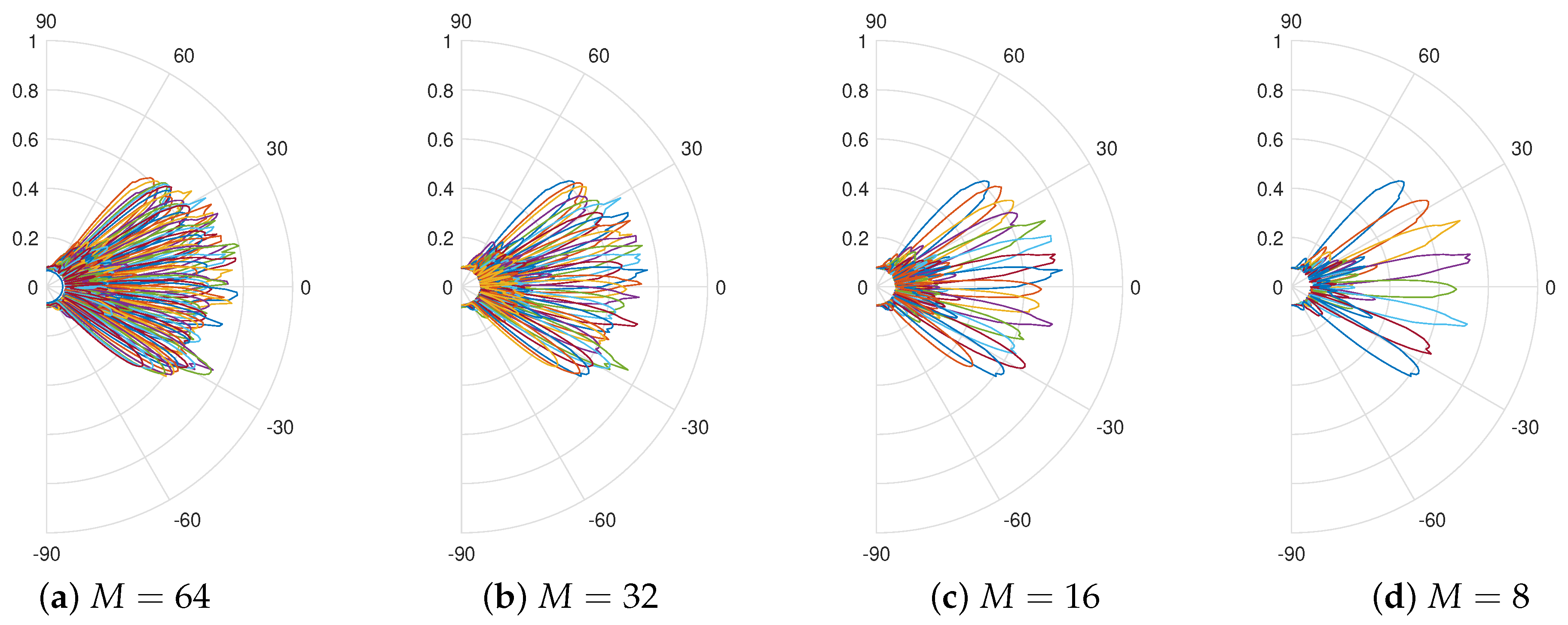
3.2. Codebook Sizes and Data Split Ratios

The main focus of this study is to investigate the impacts of codebook size and data split ratio on ML-driven beam prediction. The original dataset consists of indices $M=64$ beams. To reduce complexity and beams’ overlap, the beam codebook is downsampled from $M=64$ beams to $M\in \{32,16,8\}$ beams as shown in

Table 2. Beam Codebook Downsampling.

64 Beams	32 Beams	16 Beams	8 Beams
1, 2	1	1	1
3, 4	2
5, 6	3	2
7, 8	4
9, 10	5	3	2
11, 12	6
13, 14	7	4
15, 16	8
17, 18	9	5	3
19, 20	10
21, 22	11	6
23, 24	12
25, 26	13	7	4
27, 28	14
29, 30	15	8
31, 32	16
33, 34	17	9	5
35, 36	18
37, 38	19	10
39, 40	20
41, 42	21	11	6
43, 44	22
45, 46	23	12
47, 48	24
49, 50	25	13	7
51, 52	26
53, 54	27	14
55, 56	28
57, 58	29	15	8
59, 60	30
61, 62	31	16
63, 64	32

. We then analyze the impacts of this downsampling on the beam prediction performance (i.e., using accuracy and related metrics) for the considered ML algorithms (i.e., KNN, SVM, DT, and NB).

In Figure 4 and Figure 5, we compare the $M\in \{64,32,16,8\}$ multi-beam patterns for the ideal [21] and measured [19] cases, respectively. Unlike the ideal patterns in Figure 4 with uniform received powers and gains, the measured beam patterns in Figure 5 have non-uniform powers/gains across the beams, which indicate that the choice of beams in the downsampled codebooks may have impacts on performance. In Figure 6a–c, however, we show that the impact of beam codebook downsampling is not significant with respect to beam powers that determine the beam indices used as the ML output. Taking $M=32$ as an example, downsampling by a factor of 2 implies taking either odd-numbered $\{1,3,5,\dots ,63\}$ or even-numbered $\{2,4,6,\dots ,64\}$ beams for the 32 classes. The same patterns can be observed for $M=16$ and $M=8$. For all cases, the corresponding beam powers are comparable, except beam indexes 1 and 64 with significantly lower beam powers due to measurement design [19]. We note that the results in Figure 6 are averaged over the total 9454 samples used in this study (i.e., for Scenarios 1, 2, 5, 6, and 7 combined).

Further, this study also examines the impacts of the different data splits on the beam prediction accuracy performance of KNN, SVM, DT, and NB algorithms on the dataset. The different data splits used in the ML-based beam prediction training to testing sample ratios are as presented in Table 1 (i.e., {80:20, 70:30, 60:40}%). The hold-out partitioning method was used for data split.

3.3. ML Classification Algorithms

The ML classification algorithms considered in the study are: KNN, SVM, DT, and NB. These algorithms are fundamental ML algorithms that are widely used for classification problems, thus demonstrating their reliability and effectiveness. However, these algorithms have not been jointly applied to and compared for real-life measurement-based V2I communication datasets as carried out in this study. The four ML algorithms are briefly described as follows:

3.3.1. $\mathit{K}-$Nearest Neighbours

KNN is based on the idea that neighbors with comparable characteristics should share similar beams [16,22]. KNN algorithm is applied in the context of classifying samples based on their similarity in terms of beams using the Euclidean distance measure. With a predefined beam codebook, each beam covers a spatial direction within the FoV. Thus, KNN considers that similar or neighbor positions (using the location coordinate tuples) should have similar beams. Following the implementation in [16], the mode of the beams from $N_{knn}=5$ nearest neighbors is selected as the predicted beam. The k-smallest difference in Euclidean distances is employed as the parameter used in selecting the neighbors and predicting the beams. The true beam (ground truth) is the beam with the highest measured received power for each sample TX point. The accuracy of the algorithm is assessed by comparing its predictions to the ground truth.

3.3.2. Support Vector Machines

SVMs are effective for classification tasks. They employ kernels that turn the input data space into a higher-dimensional space. This classification approach is widely used due to its strong theoretical foundations, ability to generalize well, and adaptability to various datasets and applications. The SVMs’ effectiveness in both theory and practice has led to their broad use in the ML community [22].

In this study, we employ SVM with the Gaussian radial basis function (RBF) kernel, where the multi-class SVM (i.e., composed of multiple binary classifiers) is based on the directed acyclic graph SVM (DAG-SVM), as proposed in [23] and implemented in [24]. The RBF kernel generates nonlinear boundaries, or SVM hyperplane, between the two classes of each combination. The DAG-SVM predicts beams using only two features (location coordinate tuples in this case) and employs the one-versus-one framework to transform many two-class classifiers into a multi-class classifier for the multi-beam/multi-label prediction challenge. For an M-class problem, the DAG-SVM contains $M(M-1)/2$ classifiers, one for each pair of classes.

3.3.3. Decision Trees

DT is a well-known and commonly used classifier in classification problems [22,25]. The algorithm can handle complex datasets efficiently [26] and does not rely on data distribution assumptions [27]. A tree’s accuracy is based on its complexity [25]. DT is valued for its flexibility, efficiency with large datasets, and ability to handle diverse types of data without making strong assumptions about their distribution.

The DT algorithm predicts target beam by learning simple decision rules that it infers from the data features. The tree works as a piecewise constant approximation, and it can handle multi-class output problems. The DT classifier predicts the class of sample with the highest probability. In the event of multiple classes with the same and highest probabilities, the class with the lowest index among the classes is predicted.

3.3.4. Naïve Bayes

NB is a common classifier that applies the Bayes theorem to solve ML classification tasks [28,29]. Predicting a tuple’s membership probability is used to determine its class [28]. Before using the Bayes rule, the classifier learns the conditional probability of each attribute from the training dataset. Class predictions rely on higher posterior probability values. The naïve Bayes classifier assumes that the features are conditionally independent or unrelated for a given class.

3.4. Performance Evaluation Metrics

In this study, we employ beam prediction accuracy, precision, recall, specificity, and F1-score as performance metrics. These are commonly used evaluation metrics for ML classification problems [30,31]. Also, we show the confusion matrices for additional visual representation of the hit and miss statistics, with respect to the true and predicted beam indices. The confusion matrix is a tabular representation that summarizes the performance of a classification model by recording the number of occurrences between the true/actual classes and the predicted classes [31]. In this paper, the confusion matrices are presented such that the columns represent the model predictions, while the rows display the true classes/ground truths. The metrics are calculated for each class/beam (i.e., $\forall m\in \{1,2,\dots ,M\}$, and the results are averaged over the number of beams, M. The metrics are mathematically defined in Equations (1)–(5), respectively.

• Accuracy: This is a widely used metric for multi-class classification that can be directly derived from the confusion matrix using Equation (1). It represents the probability that the model’s prediction is accurate (i.e., how much of the predictions match the ground truths) [31].

  $$Accuracy=\sum _{m=1}^M\left({\displaystyle \frac{{\mathrm{TP}}_{\mathrm{m}}+{\mathrm{TN}}_{\mathrm{m}}}{{\mathrm{TP}}_{\mathrm{m}}+{\mathrm{TN}}_{\mathrm{m}}+{\mathrm{FP}}_{\mathrm{m}}+{\mathrm{FN}}_{\mathrm{m}}}}\right)$$

  (1)

  where TP is true positives, TN is true negatives, FP is false positives, and FN is false negatives.
• Precision: This measures the model’s ability to identify instances of a particular class correctly. It is the number of correctly classified positive samples (i.e., true positives) divided by the number of samples labeled by the system as positive, as given by Equation (2). It indicates how much we can trust the model when it predicts samples as positive.

  $$Precision={\displaystyle \frac{1}{M}}\sum _{m=1}^M\left({\displaystyle \frac{{\mathrm{TP}}_{\mathrm{m}}}{{\mathrm{TP}}_{\mathrm{m}}+{\mathrm{FP}}_{\mathrm{m}}}}\right)$$

  (2)
• Recall: This measures the model’s ability to identify all instances of a particular class. It is the number of the correctly classified positive samples divided by the number of positive samples in the data, as given by Equation (3). It measures the ability of the model to find all the positive samples in the dataset [31]. Recall is also known as the true positive rate (TPR) or sensitivity.

  $$Recall={\displaystyle \frac{1}{M}}\sum _{m=1}^M\left({\displaystyle \frac{{\mathrm{TP}}_{\mathrm{m}}}{{\mathrm{TP}}_{\mathrm{m}}+{\mathrm{FN}}_{\mathrm{m}}}}\right)$$

  (3)
• Specificity: This measures the model’s ability to identify negative instances of a particular class. It is the number of the correctly classified negative samples divided by the sum of the true negatives and false positives in the data, as given by Equation (4) [31]. Specificity is also known as the true negative rate (TNR)

  $$Specificity={\displaystyle \frac{1}{M}}\sum _{m=1}^M\left({\displaystyle \frac{{\mathrm{TN}}_{\mathrm{m}}}{{\mathrm{TN}}_{\mathrm{m}}+{\mathrm{FP}}_{\mathrm{m}}}}\right)$$

  (4)
• F1-score: This metric provides a comprehensive assessment of a classification model’s performance, taking into account both the ability to correctly identify positive instances (precision) and the ability to capture all positive instances (recall). It aggregates the precision and recall measures under the concept of harmonic mean, and its formula can be interpreted as a weighted average between precision and recall [31]. F1-score is evaluated using Equation (5). The F1-score ranges from 0 to 1, where a score of 1 indicates perfect precision and recall while a score of 0 indicates poor performance. In practice, F1-score values closer to 1 are desirable, as they indicate a well-balanced trade-off between precision and recall.

  $$F1\text{-}score={\displaystyle \frac{2·\mathrm{Precision}·\mathrm{Recall}}{\mathrm{Precision}+\mathrm{Recall}}}={\displaystyle \frac{2·\mathrm{TP}}{(2·\mathrm{TP})+\mathrm{FP}+\mathrm{FN}}}$$

  (5)

In addition, we also present the area under the receiver operating characteristic curves (AUC-ROC) to show the performance of the considered classifiers’ predictions. The ROC curve is the plot of the recall/sensitivity/TPR against the false positive rate (FPR) at different threshold values, where $FPR=1-TNR=1-specificity$. The closer the AUC to 1, the better the algorithm’s predictions, such that AUC = 1 represents a perfect model/classifier while AUC = 0.5 indicates a poor model/classifier with random guessing by the algorithm. Therefore, the closer the ROC curve to the upper left corner of the plot, the higher the accuracy of the model.

4. Performance Evaluation Results

This work focuses on multi-class classification of beam indices, in which the objective is to classify input data into one, and only one, class out of multiple non-overlapping classes. This means that each instance of input data belongs exclusively to one class out of multiple possible classes [30]. This is carried out for different data split ratios and codebook sizes as presented in Table 1 and Table 2, respectively.

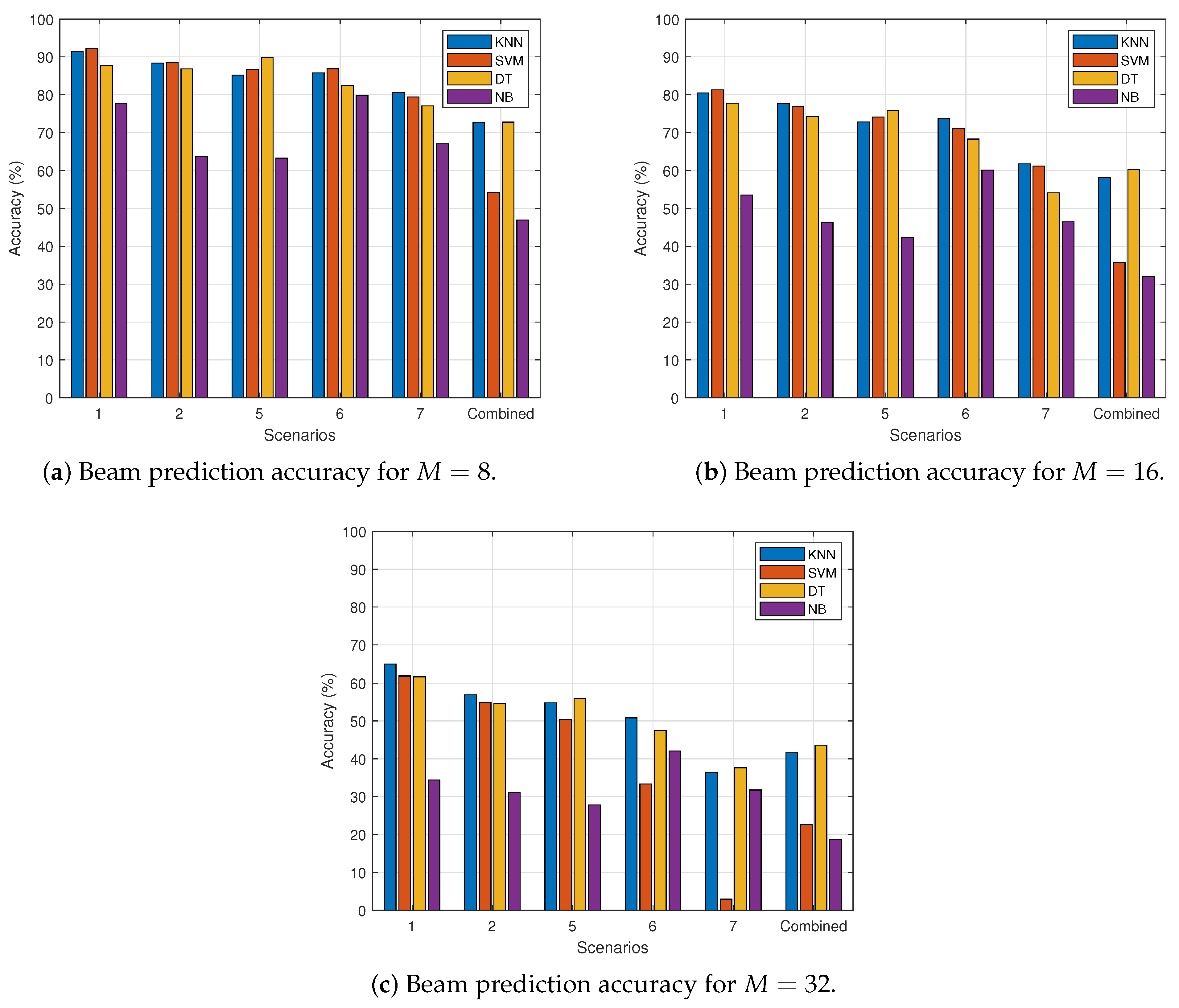
4.1. Impact of Codebook Size

The impact of codebook size $M=\{8,16,32\}$ (as given in Table 2) has been examined using the four algorithms considered in this work, across five different scenarios and the combined scenario (as given in Table 1). Figure 7a–c show the beam prediction accuracy plots of all five scenarios and the combined scenario for the {80:20}% data split for $M=8$, 16, and 32, respectively. Figure 7a–c shows that the accuracy of beam prediction decreases with increase in codebook size. Specifically, the 8-beam codebook (Figure 7a) has the best performance, while the 32-beam codebook (Figure 7c) has the least performance across the considered algorithms and scenarios. This is because the lower the number of beams in the codebook, the higher the beam pairing or prediction accuracy. Here, we note that the codebook is oversampled and the beams overlap. In systems with non-overlapping beams, covering the FoV with a lower number of beams will translate to a wider beamwidth per beam with reduced gain. Higher-dimension codebooks with narrower beams (and higher gains) will translate to a higher probability of beam misalignment and, by implication, lower beam prediction accuracies. There is, therefore, a tradeoff between the beam prediction accuracy (choice of beam) and the system performance (with respect to received power and gain, and by extension, SNR).

For scenario-by-scenario analyses for $M=8$, Figure 7a shows that SVM achieves an accuracy of over 90% in Scenario 1, followed by KNN with 90%, while DT and NB’s accuracies are 88% and 78%, respectively. In Scenario 2, SVM maintains its performance as the best algorithm, followed by DT, KNN, and NB. For Scenario 5, the best performing algorithm is DT with 90% accuracy, followed by SVM, KNN, and NB. In Scenario 6, SVM outperforms the other algorithms, followed by DT and KNN, with NB performing better than in Scenarios 2 and 5. Lastly, in Scenario 7, SVM is again the best performing algorithm, followed by DT and KNN, with NB ranking last. For $M=16$ and $M=32$, the performances follow the same trend as those of $M=8$. However, for the combined scenarios across all considered M, DT has the best performance, followed by KNN, SVM, and NB in decreasing order of performance. For $M=8$ in Figure 7a, the best accuracy results are ∼90%. For $M=16$ in Figure 7b, the best accuracy results are ∼80%, while for $M=32$ in Figure 7c, the best accuracy results are ∼60%. The results generally show higher degradation moving from $M=16$ to $M=32$ than moving from $M=8$ to $M=16$.

Overall, the beam accuracy results in Figure 7 show that the naïve Bayes algorithm consistently has the least beam prediction accuracy across the different codebooks and scenarios. This can be attributed to the fact that the longitude and latitude features are correlated or related, contrary to NB’s assumption of unrelated features. The results also reveal that the other three algorithms (KNN, SVM, and DT) have comparable performances across the codebooks and scenarios, with SVM outperforming others on the scenario-by-scenario case while DT outperforms other algorithms in the combined scenario with larger data samples than the per-scenario cases.

4.2. Impact of Dataset Split Ratio

Figure 8a–c shows the four algorithms’ beam prediction accuracy results for data splits {80:20}%, {70:30}%, and {60:40}%, for $M=8$ for the considered scenarios. The result patterns follow similar trends across the different splits and show that the data split ratios do not strongly influence the beam prediction accuracy. There are no significant changes in the results for the considered data split ratios.

4.3. Confusion Matrices for the Combined Scenario

Figure 9 shows the confusion matrices for the combined scenarios for the data split {80:20}% and $M=8$. The confusion matrices provide insights into the (mis)classification statistics of the different ML algorithms.

In Figure 9, each confusion matrix highlights the precision and recall percentages for each beam in the codebook, with precision values being displayed at the bottom of each table for each algorithm while the recall values are shown on the right sides of the confusion matrices. The classes are listed in the same order in both the rows and the columns, ensuring consistency between the true and predicted classifications. As a result, the correctly classified elements are located on the main diagonal of the confusion matrix, extending from the top left to the bottom right. These values correspond to the number of times that both the true and predicted classifications agree. By examining the values along the main diagonal, one can assess the accuracy of the classification model, as it reflects the number of correctly classified instances for each class. The off-diagonal elements provide insights into the misclassifications, showing where the model’s predictions diverge from the true classifications.

To further show the misclassification statistics,

Table 3. Misclassification percentages for KNN with $M=8$ beams.

		Predicted Beams’ Misclassification (%)
		1	2	3	4	5	6	7	8
	1	*	7.30		0.33	1.66	0.33		0.66
	2	12.77	*	12.41	0.36
Ground	3	1.16	7.54	*	10.50	0.58
Truth	4	0.55		19.67	*	18.58	1.64
Beams	5	0.48		0.96	16.35	*	15.59	1.44
	6	0.48			0.96	17.70	*	18.66	3.83
	7	0.45				3.62	16.72	*	12.67
	8	1.43					7.86	17.14	*

* represents correct classifications, omitted as the table focuses on misclassifications.

shows the percentages of the misclassified beams across the 8-beam codebook. The diagonal values are shown with * because they represent the correctly classified beams, while empty cells in Table 3 indicate no prediction for such beams. Based on the misclassification spread in the confusion matrices and on Table 3, beams have higher tendencies or probabilities to be misclassified as adjacent beams than as beams further away. Using beam 2 in the KNN 8-beam codebook as an example, out of the 25.5% misclassified beams, adjacent beam 1 and beam 3 received 12.77% and 12.41% misclassification respectively, while beam 4 that is further away from beam 2 received just 0.36% of the misclassifications. This trend is observable, to various degrees, across the considered codebooks and algorithms.

Figure 10 and Figure 11 show the confusion matrices for the combined scenarios for the data split {80:20}% for $M=16$ and $M=32$, respectively. We show the confusion matrix for $M=32$ for KNN only due to space constraints.

To further show and compare the performances of the four considered ML algorithms,

Table 4. Evaluation Metric Results for 8-beam codebook size.

Algorithm	Accuracy	Precision	Recall	Specificity	F1-Score
KNN	0.7275	0.7102	0.7098	0.9494	0.7100
SVM	0.5418	0.5288	0.5032	0.8918	0.5157
DT	0.7280	0.7119	0.7107	0.9494	0.7113
NB	0.4693	0.4849	0.4297	0.8620	0.4556

,

Table 5. Evaluation Metric Results for 16-beam codebook size.

Algorithm	Accuracy	Precision	Recall	Specificity	F1-Score
KNN	0.5820	0.5462	0.5407	0.9543	0.5435
SVM	0.3571	0.3369	0.2998	0.8823	0.3175
DT	0.6032	0.5753	0.5716	0.9582	0.5735
NB	0.3201	0.3000	0.2739	0.8564	0.2863

and

Table 6. Evaluation Metric Results for 32-beam codebook size.

Algorithm	Accuracy	Precision	Recall	Specificity	F1-Score
KNN	0.4158	0.3828	0.3623	0.9552	0.3723
SVM	0.2260	0.1686	0.1527	0.8765	0.1603
DT	0.4360	0.4035	0.3798	0.9587	0.3913
NB	0.1873	0.2013	0.1798	0.8632	0.1900

respectively show the results for codebook sizes $M=8$, 16, and 32 for the combined dataset, based on the evaluation metrics given by Equations (1)–(5) (i.e., accuracy, precision, recall, specificity, and F1-score, respectively). For all these five metrics, the closer the values to one, the better the algorithm/model’s performance. High accuracy indicates high correct predictions, while high precision shows high true positive prediction among all positive predictions by the classifier. In a similar vein, high recall shows that the model is effective at identifying positive instances, while high specificity shows that the model is effective at identifying negative instances. A higher F1-score translates to a better balance between the precision and recall values.

The results in Table 4, Table 5 and Table 6 show that the performances of the algorithms decreased as the codebook size increased. This indicates that an increase in codebook size leads to a higher rate of misclassification. Further, the results in Table 4, Table 5 and Table 6 show a beam prediction accuracy of ∼73% (for DT, $M=8$) for the best case and as low as 18% (for NB, $M=32$) for the worst case. Similarly, the F1-score statistics also reveal the best case of 0.71 and worst case value of 0.16 for the considered scenarios and codebooks. Overall, considering the performance of the four algorithms for $M=8$ beams in Table 4, the algorithm with the best performance is DT, followed by KNN, then SVM and NB. The algorithms’ performance order for $M=16$ (Table 5) and $M=32$ (Table 6) follow the same pattern as those of $M=8$, thus retaining their positions though with different performance values.

Figure 12a,b show the AUC-ROC curves for $M=8$ for DT and NB, respectively. As highlighted in Section 3.4, the closer the ROC curve is to the upper left corner of the plot (or the closer the AUC value to 1), the higher the accuracy of the model’s predictions. Also, an AUC = 0.5 (i.e., the back line on the ROC plots in Figure 12a,b with TPR = FPR) means that the model is only making random guesses. Therefore, comparing Figure 12a,b shows that DT is a better classifier than NB for the considered scenario/dataset. In Figure 12a for DT, the curves are closer to the upper left corner than those of NB in Figure 12b. Similarly, the AUCs and model operating points for beams 1–8 of DT are higher than those of NB. The DT’s average AUC is 0.89596, while that of NB is 0.82487. We have only shown AUC-ROC curves for DT (best-performing algorithm) and NB (worst-performing algorithm) and for $M=8$ only, due to space constraints. The analyses follow the same trends for KNN and SVM, and for $M=16$ and $M=32$.

On the comparison with the state-of-the-art, in

Table 7. Results’ comparison betweeen the KNN in this work and the top-1 accuracy results in [16].

Scenario	$\mathit{M}=32$		$\mathit{M}=16$		$\mathit{M}=8$
Number	[16]	This Work	[16]	This Work	[16]	This Work
1	0.7134	0.6494	0.8617	0.8050	0.9024	0.9149
2	0.6002	0.5690	0.7899	0.7778	0.8805	0.8838
5	0.5591	0.5478	0.7473	0.7283	0.8402	0.8522
6	0.6391	0.5082	0.7943	0.7377	0.9063	0.8579
7	0.4182	0.3647	0.6253	0.6177	0.7623	0.8059
Combined	0.5250	0.4159	0.5815	0.5820	0.8020	0.7275

, we compare our KNN results with the Top-1 accuracy results of Table III in [16]. The results are comparable, and the differences are due to the following:

• The number of samples or datapoints used in both works are slightly different. For example, the datapoints used in [16] for Scenarios 1, 6, and 7 are 2667, 1011, and 897, respectively (as in Figure 1 of [16]), as against the corresponding 2441, 915, and 854 samples in the publicly-released dataset used in this work, as presented in Table 2 and available in [19]. The number of samples used for Scenarios 2 and 5 are unavailable in [16].
• The combined results in [16] are averaged over nine scenarios, while the combined results in this work are averaged over five scenarios.
• In [16], the GPS coordinates are employed directly as ML features, while the coordinates are converted first to cartesian coordinates in this work as part of the preprocessing steps before being used as the ML features.

As also noted in [16], the performance results depend to a large extent on the specific scenario under consideration as well as on the number of samples, as can be observed in Table 7, and also depend on the employed algorithm.

In summary, the performance results, on the one hand, reveal realistic values achievable from real-life experimental datasets as against the performance with simulated datasets. On the other hand, the performance results point in the direction that position-only data may not be sufficient for high accuracies (typically more than 95%) needed to support the ambitious demands of 5G and beyond networks, particularly for high mobility vehicular use cases. The position data can therefore be combined with other sensor data (such as LiDAR, radar, and camera) to improve the beam accuracies and the overall network performance.

5. Conclusions and Future Directions

This study examined the effects of codebook size and dataset split ratios on the performance of four ML algorithms, namely KNN, SVM, DT, and NB, for GPS-aided mmWave V2I beam prediction. The datasets used in this study were based on the real-world mmWave V2I DeepSense6G experimental datasets. The results show that the performance of the ML algorithms declines as the codebook size increases. This means that lower codebook sizes (i.e., with lower number of beams) lead to more accurate beam pairing predictions as the probability of beam alignment is higher. Additionally, the algorithms are mostly unaffected by the data split ratios used in the ML algorithms, such that 20, 30, and 40% testing ratios of the dataset give comparable beam prediction accuracy results. Generally, for the combined scenario, the results show that DT outperform the other classifiers, followed by KNN, SVM, and NB. The future research direction is to investigate other ML algorithms, explore the impacts of other system parameters, and consider multi-modal approaches employing a combination of sensor data such as LiDAR, radar, and camera in addition to the position data employed as ML features in this study.

References

1. Ballesteros, C.; Montero, L.; Ramírez, G.A.; Jofre-Roca, L. Multi-antenna 3D pattern design for millimeter-wave vehicular communications. Veh. Commun. 2022, 35, 100473. [Google Scholar] [CrossRef]
2. Decarli, N.; Guerra, A.; Giovannetti, C.; Guidi, F.; Masini, B.M. V2X Sidelink Localization of Connected Automated Vehicles. IEEE J. Sel. Areas Commun. 2024, 42, 120–133. [Google Scholar] [CrossRef]
3. Heng, Y.; Andrews, J.G. Machine Learning-Assisted Beam Alignment for mmWave Systems. In Proceedings of the 2019 IEEE Global Communications Conference (GLOBECOM), Waikoloa, HI, USA, 9–13 December 2019. [Google Scholar]
4. Va, V.; Shimizu, T.; Bansal, G.; Heath, R.W. Online Learning for Position-Aided Millimeter Wave Beam Training. IEEE Access 2019, 7, 30507–30526. [Google Scholar] [CrossRef]
5. Busari, S.A.; Khan, M.A.; Huq, K.M.S.; Mumtaz, S.; Rodriguez, J. Millimetre-wave massive MIMO for cellular vehicle-to-infrastructure communication. IET Intell. Transp. Syst. 2019, 13, 983–990. [Google Scholar] [CrossRef]
6. Attaoui, W.; Bouraqia, K.; Sabir, E. Initial Access & Beam Alignment for mmWave and Terahertz Communications. IEEE Access 2022, 10, 35363–35397. [Google Scholar] [CrossRef]
7. Sun, C.; Zhao, L.; Cui, T.; Li, H.; Bai, Y.; Wu, S.; Tong, Q. AI model Selection and Monitoring for Beam Management in 5G-Advanced. IEEE Open J. Commun. Soc. 2024, 5, 38–40. [Google Scholar] [CrossRef]
8. Choi, J.; Va, V.; Gonzalez-Prelcic, N.; Daniels, R.; Bhat, C.R.; Heath, R.W. Millimeter-Wave Vehicular Communication to Support Massive Automotive Sensing. IEEE Commun. Mag. 2016, 54, 160–167. [Google Scholar] [CrossRef]
9. Yang, Z.; Chen, M.; Wong, K.; Poor, H.V.; Cui, S. Federated Learning for 6G: Applications, Challenges, and Opportunities. Engineering 2022, 8, 33–41. [Google Scholar] [CrossRef]
10. Ali, S.; Saad, W.; Rajatheva, N.; Chang, K.; Steinbach, D.; Sliwa, B.; Wietfeld, C.; Mei, K.; Shiri, H.; Zepernick, H.; et al. 6G White Paper on Machine Learning in Wireless Communication Networks. arXiv 2020, arXiv:2004.13875. [Google Scholar]
11. Burghal, D.; Abbasi, N.A.; Molisch, A.F. A Machine Learning Solution for Beam Tracking in mmWave Systems. In Proceedings of the 2019 53rd IEEE Asilomar Conference on Signals, Systems, and Computers, Pacific Grove, CA, USA, 3–6 November 2019; pp. 173–177. [Google Scholar]
12. Wang, Y.; Klautau, A.; Ribero, M.; Soong, A.C.K.; Heath, R.W. MmWave Vehicular Beam Selection with Situational Awareness Using Machine Learning. IEEE Access 2019, 7, 87479–87493. [Google Scholar] [CrossRef]
13. Arvinte, M.; Tavares, M.; Samardzija, D. Beam Management in 5G NR using Geolocation Side Information. In Proceedings of the 2019 53rd IEEE Annual Conference on Information Sciences and Systems (CISS), Baltimore, MD, USA, 20–22 March 2019; pp. 1–6. [Google Scholar]
14. Jiang, S.; Charan, G.; Alkhateeb, A. LiDAR Aided Future Beam Prediction in Real-World Millimeter Wave V2I Communications. IEEE Wirel. Commun. Lett. 2023, 12, 212–216. [Google Scholar] [CrossRef]
15. Echigo, H.; Cao, Y.; Bouazizi, M.; Ohtsuki, T. A Deep Learning-Based Low Overhead Beam Selection in mmWave Communications. IEEE Trans. Veh. Technol. 2021, 70, 682–691. [Google Scholar] [CrossRef]
16. Morais, J.; Bchboodi, A.; Pezeshki, H.; Alkhateeb, A. Position-Aided Beam Prediction in the Real World: How Useful GPS Locations Actually are? In Proceedings of the 2023 IEEE International Conference on Communications, Rome, Italy, 28 May–1 June 2023; pp. 1824–1829. [Google Scholar]
17. Charan, G.; Osman, T.; Hredzak, A.; Thawdar, N.; Alkhateeb, A. Vision-Position Multi-Modal Beam Prediction Using Real Millimeter Wave Datasets. In Proceedings of the 2022 IEEE International Conference on Communications, Austin, TX, USA, 10–13 April 2022; pp. 2727–2731. [Google Scholar] [CrossRef]
18. Makadia, O.B.; Patel, D.K.; Shah, K.D.; Raval, M.S.; Zaveri, M.; Merchant, S.N. Millimeter-Wave Vehicle-to-Infrastructure Communications for Autonomous Vehicles: Location-Aided Beam Forecasting in 6G. In Proceedings of the 2024 16th International Conference on COMmunication Systems & NETworkS (COMSNETS), Bengaluru, India, 3–7 January 2024; pp. 1100–1105. [Google Scholar] [CrossRef]
19. A Large-Scale Real-World Multi-Modal Sensing and Communication Dataset for 6G Deep Learning Research. Available online: https://www.deepsense6g.net/ (accessed on 10 April 2024).
20. Alkhateeb, A.; Charan, G.; Osman, T.; Hredzak, A.; Morais, J.; Demirhan, U.; Srinivas, N. DeepSense 6G: A Large-Scale Real-World Multi-Modal Sensing and Communication Dataset. IEEE Commun. Mag. 2023, 61, 122–128. [Google Scholar] [CrossRef]
21. Roberts, I.P. MIMO for MATLAB: A Toolbox for Simulating MIMO Communication Systems in MATLAB. January 2021. Available online: http://mimoformatlab.com (accessed on 15 May 2024).
22. Cervantes, J.; Garcia-Lamont, F.; Rodrıguez-Mazahua, L.; Lopez, A. A comprehensive survey on support vector machine classification: Applications, challenges and trends. Neurocomputing 2020, 408, 189–215. [Google Scholar] [CrossRef]
23. Platt, J.C.; Cristianini, N.; Shawe-Taylor, J. Large Margin DAGs for Multiclass Classification. In Advances in Neural Information Processing Systems 12 (NIPS 1999); MIT Press: Cambridge, MA, USA, 1999; pp. 547–553. [Google Scholar]
24. Pilario, K.E. Binary and Multi-Class SVM. MATLAB Central File Exchange. Available online: https://www.mathworks.com/matlabcentral/fileexchange/65232-binary-and-multi-class-svm (accessed on 10 April 2024).
25. Rokach, L.; Maimon, O. Decision Trees. In Data Mining and Knowledge Discovery Handbook; Springer: New York, NY, USA, 2005; pp. 165–192. [Google Scholar]
26. Song, Y.Y.; Lu, Y. Decision tree methods: Applications for classification and prediction. Shanghai Arch. Psychiatry 2015, 45, 130–135. [Google Scholar]
27. Fletcher, S.; Islam, M.Z. Decision Tree Classification with Differential Privacy: A Survey. ACM Comput. Surv. 2019, 52, 83. [Google Scholar] [CrossRef]
28. Guleria, K.; Sharma, S.; Kumar, S.; Tiwari, S. Early prediction of hypothyroidism and multiclass classification using predictive machine learning and deep learning. Meas. Sens. 2022, 24, 100482. [Google Scholar] [CrossRef]
29. Farid, D.M.; Rahman, M.M.; Al-Mamuny, M.A. Efficient and scalable multi-class classification using Naïve Bayes tree. In Proceedings of the 2014 International Conference on Informatics, Electronics & Vision (ICIEV), Dhaka, Bangladesh, 23–24 May 2014; pp. 1–4. [Google Scholar]
30. Sokolova, M.; Lapalme, G. A systematic analysis of performance measures for classification tasks. Inf. Process. Manag. 2009, 45, 427–437. [Google Scholar] [CrossRef]
31. Margherita, G.; Enrico, B.; Giorgio, V. Metrics for Multi-Class Classification: An Overview. arXiv 2020, arXiv:2008.05756. [Google Scholar]
Figure 1. Scenario 6 layout showing the vehicle’s (TX) positions on the lanes (i.e., colored circles where the colors represent the beam indices) and the RX/AP’s position and its field of view (Reproduced from https://www.wi-lab.net/research/position-aided-prediction-paper-how-useful-gps-positions-actually-are/, accessed on 1 May 2024).
Electronics 13 02656 g001
Figure 2. Received powers vs. Beam Indices for selected Scenario 6 data samples (64-beam codebook).
Electronics 13 02656 g002
Figure 3. Study methodology flowchart.
Electronics 13 02656 g003
Figure 4. Ideal multi-beam patterns for M { 64 , 32 , 16 , 8 } (Generated using MATLAB code from [21]).
Electronics 13 02656 g004
Figure 5. Measured multi-beam patterns for M { 64 , 32 , 16 , 8 } (Generated using data and MATLAB code from [19]).
Electronics 13 02656 g005
Figure 6. Received powers against beam indices for different for M { 32 , 16 , 8 } downsampling.
Electronics 13 02656 g006
Figure 7. Beam Prediction accuracy comparison for different codebook sizes and 80:20% dataset split.
Electronics 13 02656 g007
Figure 8. Beam Prediction accuracy comparison for different dataset splits for M = 8 .
Electronics 13 02656 g008
Figure 9. Confusion Matrices for the Combined Scenario with the M = 8 beams (Blue color represents correct classifications while orange represents misclassifcations; the darker the color tone, the higher the value).
Electronics 13 02656 g009
Figure 10. Confusion matrices for the Combined Scenario with M = 16 and 80:20% split (Blue color represents correct classifications while orange represents misclassifcations; the darker the color tone, the higher the value).
Electronics 13 02656 g010
Figure 11. KNN Confusion Matrix for the Combined Scenario with M = 32 and 80:20% split (Blue color represents correct classifications while orange represents misclassifcations; the darker the color tone, the higher the value).
Electronics 13 02656 g011
Figure 12. AUC-ROC curves for (a) DT and (b) NB for the Combined Scenario with M = 8 .
Electronics 13 02656 g012