Article

Few-Shot Image Segmentation Using Generating Mask with Meta-Learning Classifier Weight Transformer Network

by
Jian-Hong Wang
1,†,
Phuong Thi Le
2,†,
Fong-Ci Jhou
3,
Ming-Hsiang Su
4,*,
Kuo-Chen Li
5,*,
Shih-Lun Chen
6,
Tuan Pham
7,
Ji-Long He
1,
Chien-Yao Wang
8,
Jia-Ching Wang
9 and
Pao-Chi Chang
3
1
School of Computer Science and Technology, Shandong University of Technology, Zibo 255000, China
2
Department of Computer Science and Information Engineering, Fu Jen Catholic University, New Taipei City 24205, Taiwan
3
Department of Communication Engineering, National Central University, Taoyuan City 320314, Taiwan
4
Department of Data Science, Soochow University, Taipei City 10048, Taiwan
5
Department of Information Management, Chung Yuan Christian University, Taoyuan City 320314, Taiwan
6
Department of Electronic Engineering, Chung Yuan Christian University, Taoyuan City 320314, Taiwan
7
Faculty of Digital Technology, University of Technology and Education—The University of Danang, Danang 550000, Vietnam
8
Institute of Information Science, Academia Sinica, Taipei 115201, Taiwan
9
Department of Computer Science and Information Engineering, National Central University, Taoyuan City 320314, Taiwan
*
Authors to whom correspondence should be addressed.
These authors contributed equally to this work.
Electronics 2024, 13(13), 2634; https://doi.org/10.3390/electronics13132634
Submission received: 5 May 2024 / Revised: 14 June 2024 / Accepted: 26 June 2024 / Published: 4 July 2024
(This article belongs to the Special Issue Intelligent Big Data Analysis for High-Dimensional Internet of Things)

Abstract

:
With the rapid advancement of modern hardware technology, breakthroughs have been made in many areas of artificial intelligence research, leading to the direction of machine replacement or assistance in various fields. However, most artificial intelligence or deep learning techniques require large amounts of training data and are typically applicable to a single task objective. Acquiring such large training datasets can be particularly challenging, especially in domains like medical imaging. In the field of image processing, few-shot image segmentation is an area of active research. Recent studies have employed deep learning and meta-learning approaches to enable models to segment objects in images with only a small amount of training data, allowing them to quickly adapt to new task objectives. This paper proposes a network architecture for meta-learning few-shot image segmentation, utilizing a meta-learning classification weight transfer network to generate masks for few-shot image segmentation. The architecture leverages pre-trained classification weight transfers to generate informative prior masks and employs pre-trained feature extraction architecture for feature extraction of query and support images. Furthermore, it utilizes a Feature Enrichment Module to adaptively propagate information from finer features to coarser features in a top-down manner for query image feature extraction. Finally, a classification module is employed for query image segmentation prediction. Experimental results demonstrate that compared to the baseline using the mean Intersection over Union (mIOU) as the evaluation metric, the accuracy increases by 1.7% in the one-shot experiment and by 2.6% in the five-shot experiment. Thus, compared to the baseline, the proposed architecture with meta-learning classification weight transfer network for mask generation exhibits superior performance in few-shot image segmentation.

1. Introduction

Humans possess high intelligence and exhibit keen senses in both vision and hearing, enabling rapid learning and identification of information received by the eyes and ears. However, achieving precise outcomes in high-precision instrument operations often requires the assistance of relevant programs or instruments, as human capabilities alone may fall short. Therefore, there is a desire to leverage machines to replace human labor and reduce labor costs. With the development of artificial intelligence (AI) technology, various fields have delved into AI research, leading to the emergence of machine learning and deep learning techniques applied in real-life scenarios. In recent years, there has been groundbreaking progress in deep learning and machine learning, particularly in the research of visual imagery and audio, creating a trend of deep learning research.
Among the numerous topics in deep learning research, visual imagery processing is one of the most extensively studied areas. Many researchers utilize deep neural network (DNN) models to explore applications such as classification, segmentation, and recognition, which are closely related to daily life, including facial recognition, calcaneus fracture detection, medical image segmentation, iris image segmentation, animal species classification, guitar playing technique recognition, sound recognition, and speech recognition [1,2,3,4,5,6,7,8]. These studies typically require large amounts of training data and annotations to train accurate models. Therefore, the investigation of how to train deep learning models with limited annotated data as well as feature generalization [9] is crucial to align with the scarcity of data available for real-world applications. In response to this challenge, research areas such as meta-learning and few-shot learning have emerged, aiming to train deep learning models effectively with limited training data. Some research applies pseudo-labeling to enhance the data of certain classes, improving the robustness of few-shot learning [10,11,12]. Other research leverages better generalization performance from the robustness of meta-learning.
In this paper, we focus on utilizing meta-learning for few-shot semantic segmentation of images. This paper clearly described our few-shot image segmentation system [13].
Traditional deep training models for image segmentation often rely on extensive training data to achieve satisfactory model performance. However, real-world applications may not provide such abundant training data. Therefore, the question of how to utilize meta-learning for few-shot image segmentation remains an important topic for research and exploration.
In today’s landscape of high-performing deep learning models for image and speech processing, a significant amount of annotated training data is required to train a model that excels at specific task objectives. However, preparing large amounts of annotated data before training a model consumes considerable resources such as time, manpower, and finances. Moreover, trained models are limited to the tasks or categories they were trained on, highlighting the need for a solution to this challenge. Combining few-shot image segmentation training with meta-learning provides a promising approach to address these issues.
However, in training few-shot image segmentation models, the key objective is to enhance accuracy by utilizing only one correctly annotated image or a small set of five annotated images. Additionally, after training a few-shot image segmentation model, integrating meta-learning to enable the model to perform well on new category targets is crucial. This paper aims to pursue these objectives. Furthermore, comparing the proposed architecture with other meta-learning integrated few-shot image segmentation models aims to demonstrate its superior performance.
In summary, the research objectives and focuses of this paper are as follows:
  • Proposing improvements to enhance the accuracy of few-shot image segmentation models.
  • Integrating meta-learning with few-shot image segmentation models to enable excellent performance on new category targets.

2. Attention Mechanism

The attention mechanism was first introduced in 2014 by D. Bahdanau in the Seq2Seq architecture [14], initially applied to the problem of neural machine translation. In 2017, Google introduced the “Transformer” network architecture [15], which achieved a breakthrough in the field of natural language processing (NLP), attracting increasing attention from researchers and leading to the incorporation of the attention mechanism in various research fields. This section will introduce different methods of the attention mechanism [15].

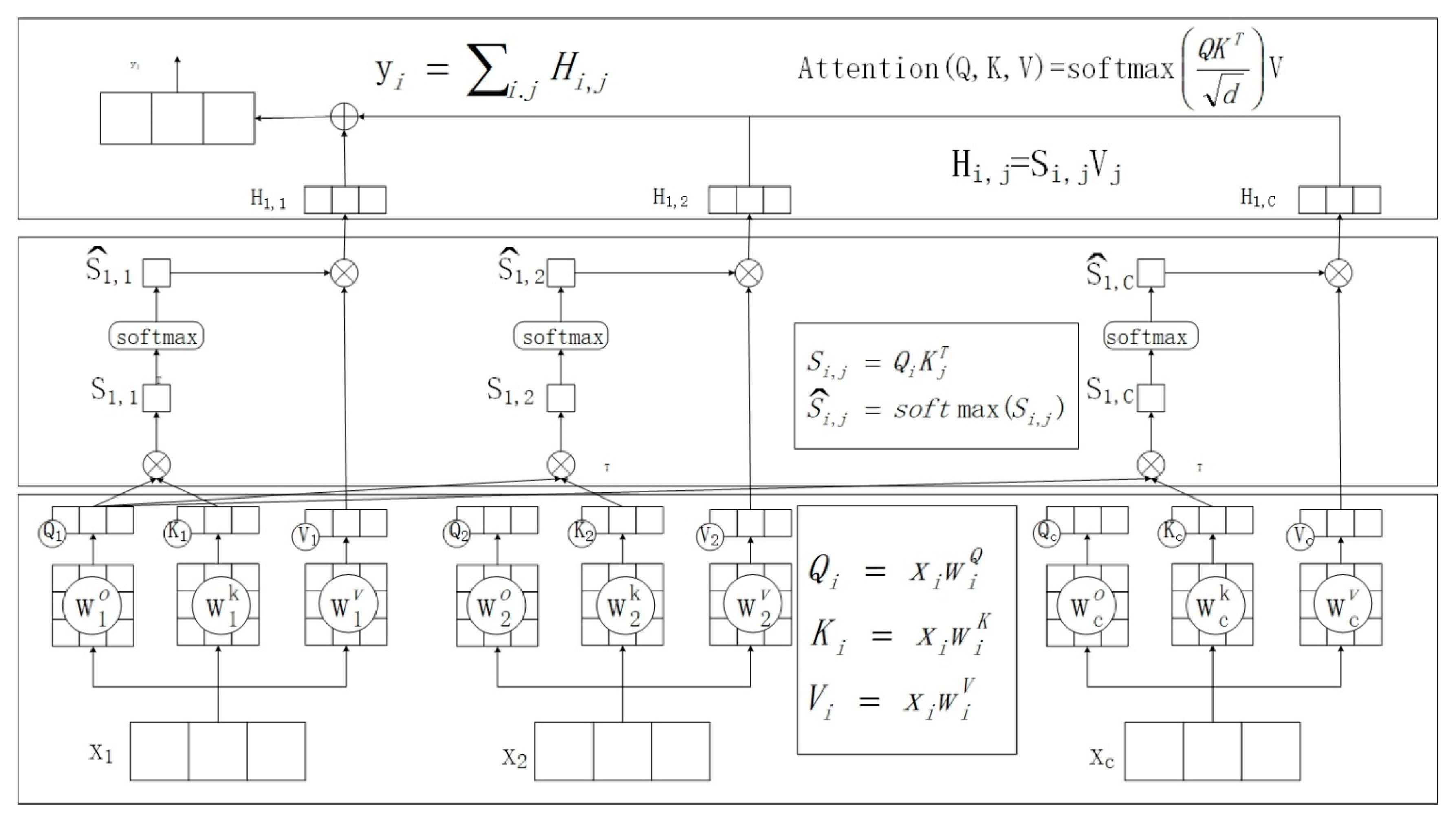
2.1. Self-Attention Mechanism

The Seq2Seq network architecture can be seen as comprising an Encoder and a Decoder. During training, no intermediate outputs are generated; instead, the prediction results are directly outputted after inputting the data. Therefore, such models are often composed of RNNs. However, RNN models exhibit sequential computation, requiring the processing of the previous data before handling the current data. As the sequence lengthens, RNN models tend to forget past information. To address this issue, the self-attention mechanism was proposed. The main formula of the self-attention mechanism, as shown in Equation (1), consists of three inputs: Q (Query), K (Key), and V (Value). Each signal is multiplied by different weights, denoted as W q , W k , and W v , which are initially set by random initialization during training. Query and Key calculate similarity at different time steps, while Value represents the input feature vectors of each signal.
The process is illustrated in Figure A1. Given input data x 1 ,   x 2 , ,   x c , each input calculates Q, K, and V separately. When computing the Attention Score for x 1 , it multiplies the Q of x 1 by its own K and the K of other inputs, then normalizes the result by dividing by d . Afterward, it multiplies the matching degree of x 1 with other inputs by their respective V and sums them up to output y 1 .
A t t e n t i o n Q , K , V = s o f t m a x Q K T d V

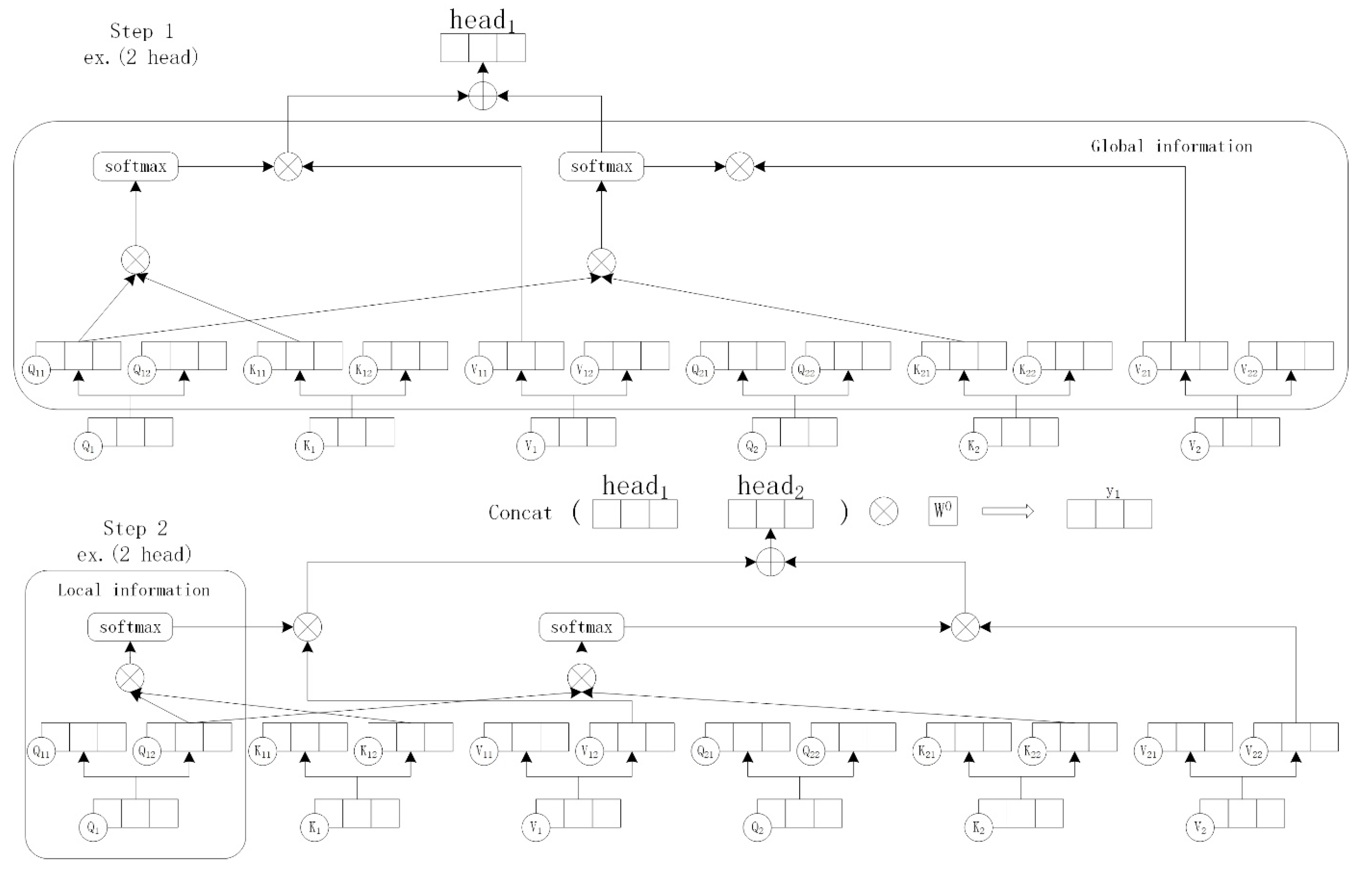
2.2. Multi-Head Self-Attention Mechanism

The Multi-Head Self-Attention Mechanism (MHSA) is an extension of the self-attention mechanism. It involves partitioning the original Q , K and V of each input into multiple sets, forming multiple different spaces beneath each input. This allows the model to learn a wider range of contextual information, as represented by Equations (2) and (3). As illustrated in Figure A2, taking two heads as an example, the original Q , K and V are divided into two sets each to perform self-attention mechanism computation. Finally, the outputs of the two heads are concatenated together and multiplied by weights for output.
M u l t i H e a d Q , K , V = C o n c a t h e a d 1 , h e a d 2 , , h e a d n W 0
w h e r e   h e a d i = A t t e n t i o n Q W i Q , K W i K , V W i V

3. Meta-Learning and Few-Shot Learning Background

With the development of deep learning, significant breakthroughs have been achieved in the fields of image and speech processing, and deep learning models have already demonstrated outstanding performance on specific tasks. However, there is still a gap between deep learning models and humans. For example, when learning new things, humans can learn from a few examples, and our instinctive learning mechanisms enable us to quickly leverage previous knowledge to learn about new problems in different environments. Therefore, in order to enable models to learn how to learn, the concept of meta-learning has been developed.
In few-shot learning, the goal is also to learn models for new tasks with only a small number of labeled samples, making it related to the concept of meta-learning. Moreover, in the current fields of image processing and speech processing, training a model that performs well on a single task requires a large amount of annotated data. Acquiring such data entails significant time, manpower, and financial costs. Thus, the topic of few-shot learning has been proposed, aiming to train models with a small amount of labeled data to achieve good performance on new tasks.
This section will introduce methods related to meta-learning, few-shot learning, and relevant literature on image segmentation.

3.1. Meta-Learning

Meta-learning, also known as “learning to learn”, involves teaching models how to utilize past knowledge and experience to learn new tasks. Meta-learning can facilitate rapid learning in few-shot training scenarios, making it commonly used to address few-shot training problems. This section will discuss different approaches to meta-learning.

3.1.1. Gradient-Based Meta-Learning

In this subsection, we introduce a method proposed by Chelsea Finn et al. in 2017, called Model-Agnostic Meta-Learning (MAML) [16]. From the name of this method, it can be inferred that it is a “model-agnostic” meta-learning framework. The meta-learning framework proposed can be applied to any deep learning model based on gradient descent algorithms and can learn various task objectives.
Before introducing the MAML method, we need to explain the part of training and testing data in meta-learning. In conventional deep learning, training data and testing data are referred to as meta-training and meta-testing in meta-learning, respectively. Then, within these two sets, there are subsets referred to as training data, also known as support data, and testing data, also known as query data.
Algorithm 1 is the Model-Agnostic Meta-Learning Algorithm [16]:
Algorithm 1. Model-Agnostic Meta-Learning Algorithm:
Require: p T : distribution over task
Require: a , β :step size hyperparameters
 1: randomly initialize 0
 2: while not done do
 3:  Sample batch of task T i   p T
 4:  for all T i do
 5:   Sample K data points D = { x j , y j } from T i
 6:   Evaluate θ L T i f θ using D
 7:   Compute adapted parameters with gradient descent: θ i = θ α θ L T i f θ
 8:   Sample data points D i = { x j , y j } from T i , for the meta-update
 9:   end for
10:  Update θ θ β θ T i   p T L T i f θ i using each D_i^’
11: end while
Now, we introduce the algorithm of MAML. It is mainly divided into three major steps:
  • Sample batch of tasks: Randomly sample one or more batches of training tasks from meta-training, and then sample training data from each task.
  • Evaluate gradient and compute adapted parameters: Compute the gradient for each task and its corresponding labels in the training data and update the model parameters θ i accordingly.
  • Update the model: With the newly updated model parameters θ i for each task using the meta-training data, validate using the meta-training test data sampled calculate the loss for all tasks, update the original model parameters, and store the model.

3.1.2. Metric-Based Meta-Learning

The following subsection will introduce metric-based meta-learning. In 2017, Prototypical Networks proposed by Jake Snell et al. [17] calculated the average features of each class in the support data and classified the query data using the nearest-centroid method.
N is the total number of samples in meta-training, K is the number of categories in meta-training, N C is the number of categories after one episode of the algorithm, N S is the training data of meta-training (support examples), and N Q is the testing data of meta-training (query examples). After sampling the training data, the equation “Compute prototype from support examples” calculates the mean vector of the embedded features for each class in the training data of meta-training (support examples). Then, the “Update loss” equation calculates the distance between the testing data of training data (query examples) and the previously computed mean vector c k using a distance function (d), which can be Euclidean distance or cosine distance. Finally, the calculated loss is used to update the overall model parameters.
Algorithm 2 is the Prototypical Networks Algorithm [17]:
Algorithm 2. Training Episode Loss Computation for Prototypical Networks. N is the Number of Examples in the Training Set, K is the Number of Classes in the Training Set, Nc < K is the Number of Classes per Episode, Ns is the Number of Support Examples per Class, NQ is the Number of Query Examples per Class. RANDOMSAMPLE(S, N) Denotes a Set of N Elements Chosen Uniformly at Random from Set S, without Replacement.
Input: Training set D = { x 1 , y 1 , . . . , x N , y N } , where each y i { 1 , . . . , K } . Dk denotes the subset of D containing all elements x i , y i such that y i = k .
Output: The loss J for a randomly generated training episode.
 1: V R A N D O M S A M P L E { 1 , . . . , K } , N c  Select class indices for episode
 2: for k in { 1 , . . . , N C } do
 3:    S k R A N D O M S A M P L E D V k , N S  Select support examples
 4:    Q k R A N D O M S A M P L E D V k / S S , N Q  Select query examples
 5:    c k 1 N C x i , y i S k f Φ x i  Compute prototype from support examples
 6: end for
 7: J 0
 8: for k in { 1 , . . . , N C } do Initialize loss
 9:   for x , y in Q k do
10:     J J + 1 N C N Q d f Φ x , c k + l o g k e x p d f Φ x , c k  Update loss
11:  end for
12: end for

3.2. Few-Shot Learning

Few-shot learning, as the name suggests, is about learning models for new categories with only a few labeled samples. It is typically expressed in K-shot experiments, where during model training, only K-labeled samples are used. In classification tasks, it is represented as N-way, K-shot, such as a five-way, five-shot classification task, meaning there are five classes with only five labeled samples per class.
Many people have used meta-learning methods to address few-shot learning tasks. However, the definition of few-shot learning in the context of meta-learning training differs slightly. Taking the MAML algorithm described in Section 3.1.1 as an example, in a five-way, five-shot experiment, a task is first sampled from the training data of meta-training, using five labeled training data (support data) to train a temporary model. Then, 15 labeled testing data (query data) per class are sampled from the testing data of meta-training to perform the final model update. After obtaining a trained model, the process enters the meta-testing stage. Using the model updated in the meta-training stage, a five-way, five-shot task is sampled from the training data of meta-testing, and again, five labeled training data (support data) are used to train a temporary model. Then, one unlabeled testing data (query data) is sampled from the testing data of meta-testing and input into the trained temporary model for prediction.
Therefore, the few-shot training problem solved using meta-learning is consistent with the previous few-shot learning settings only in the meta-testing stage. Most current few-shot learning methods adopt meta-learning approaches, primarily focusing on classification tasks using gradient descent methods like MAML and metric-based approaches like Prototypical Networks [17]. There are also other metric-based meta-learning methods for few-shot training, such as [18,19,20,21].

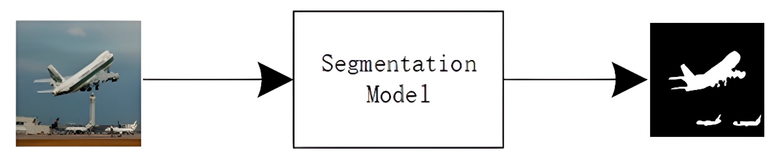
3.3. Image segmentation

3.3.1. Semantic Segmentation

Semantic segmentation is a fundamental topic in image segmentation, which involves classifying all pixels in an image, as shown in Figure 1. In 2014, Long, J. et al. proposed Fully Convolutional Networks (FCN) [22], which replaced fully connected layers with convolutional layers to develop semantic segmentation tasks, laying an important foundation for subsequent semantic segmentation tasks.
In the subsequent development of semantic segmentation models, the importance of receptive fields has been recognized. Therefore, dilation convolutions were introduced by Yu, F. et al. in 2016 [23] and were utilized in the DeepLab model proposed by Chen, L. et al. in 2018 [24] to enlarge the receptive field. Many semantic segmentation models that followed also adopted architectures based on encoders and decoders. For instance, U-net [25], proposed by Ronneberger, O. et al. in 2015, falls into this category. In many semantic segmentation studies, extracting contextual information has proven to be beneficial. ParseNet [26], introduced by Liu, W. et al. in 2015, was the first to utilize global pooling to extract global features. Subsequently, in 2017, Zhao, H. et al. proposed PSPNet [27], which employed the Pyramid Pooling Module (PPM) to combine context features extracted using pooling of different sizes. Additionally, DeepLab developed the Atrous Spatial Pyramid Pooling Module (ASPP), which consists of filters with different dilation rates.
The aforementioned methods are suitable for training on large sample classes. They are not specifically designed to handle rare and unseen categories. Without fine-tuning, they may also struggle to adapt.

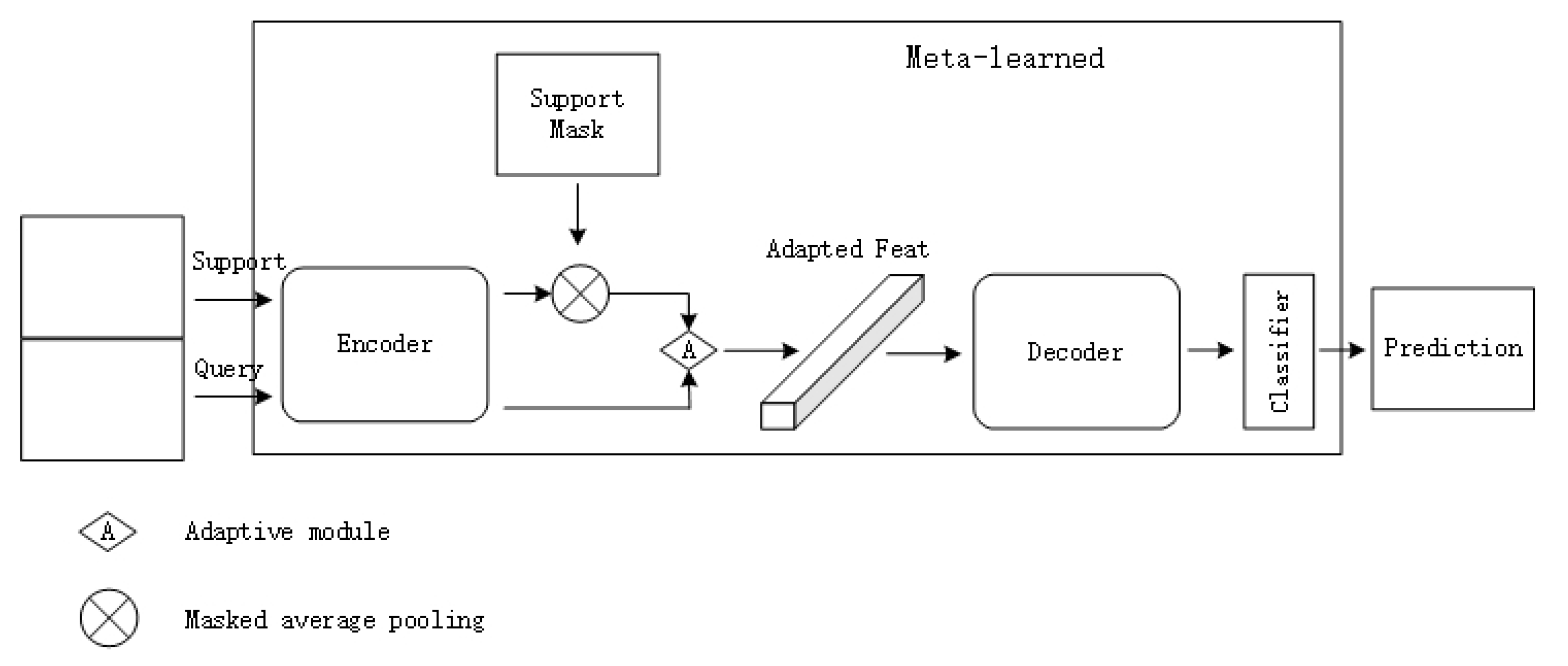
3.3.2. Few-Shot Image Segmentation

Few-shot image segmentation involves training a model with only a few training samples for the purpose of segmenting images, enabling the trained model to be applicable to segmentation tasks of new classes. Similar to the meta-learning techniques introduced in Section 3.1 and Section 3.2, meta-learning has also been introduced into few-shot semantic image segmentation to address the same few-shot learning problem.
In 2017, the OSLSM [28] model proposed by Shaban, A. et al. addressed few-shot segmentation problems by training weights for classifiers for each category. In general, semantic segmentation systems consist of three parts: an encoder, a decoder, and a classifier. To integrate meta-learning, existing models typically associate features from support data and query data images obtained from the encoder, and then update all three components by minimizing the loss by measuring the difference between predictions and ground truth (as shown in Figure 2). For example, in 2018, Dong, N. et al. applied the Prototype Network [17] to few-shot image segmentation tasks and proposed the PL [29] network architecture, which learns prototypes for each category and calculates cosine similarity between targets and prototypes for prediction. Subsequently, many models have emerged. For instance, PANet [30] introduced prototype alignment regularization for bidirectional prototype learning, enabling the model to learn identical prototypes and achieve better performance. However, CANet [31] used an iterative optimization module when connecting query data features and support data features to optimize results. Then, in 2017, PPNet [32], proposed by Lin, G. et al., emphasized the importance of fine-grained features and introduced partial perception prototypes.
Based on the aforementioned few-shot semantic segmentation models, meta-learning is incorporated to address the few-shot learning problem, enabling the trained models to adapt to image segmentation applications of new categories.

4. Experimental Results

This study aims to achieve few-shot image segmentation using meta-learning. A deep learning approach is employed to construct a network model capable of semantic segmentation with a small number of training samples while maintaining excellent segmentation accuracy when segmenting images of new categories. Two experimental architectures are designed based on different network architectures. Among them, the model proposed in this paper, based on meta-learning for few-shot image segmentation, demonstrates good image segmentation accuracy when presented with images of categories not seen during training.
This section mainly introduces the model proposed in this paper, which is based on meta-learning for few-shot image segmentation. Firstly, we briefly describe the two experimental architecture processes designed in this paper. These include the Continual Weight Transfer (CWT) architecture [33], which updates part of the network, and the experimental architecture proposed in this paper, which incorporates meta-learning for few-shot image segmentation, featuring a meta-learning classification weight transfer network for generating masks in few-shot image segmentation experiments. Next, we introduce the feature extraction methods and the classification weight transfer used in the two experiments. We then discuss the prior mask generation method and the Feature Enrichment Module used in the second experimental method. Finally, we introduce the loss functions used in the two experimental methods.

4.1. System Architecture

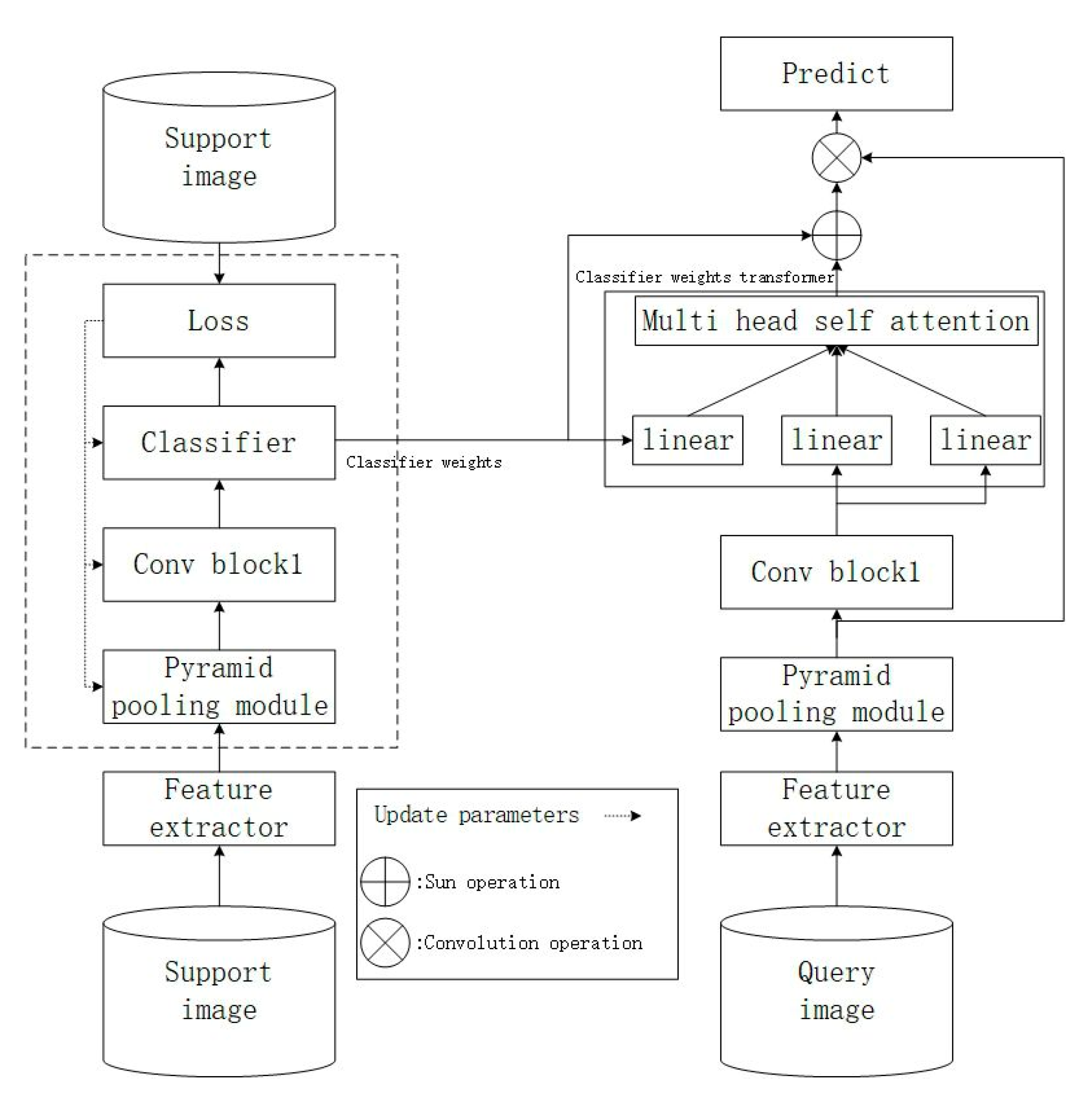
4.1.1. CWT Architecture with Partial Network Updates

The first experimental architecture designed in this paper is an improvement upon the CWT (Continual Weight Transfer) architecture proposed by Lu, Z. et al. [33]. The flowchart is depicted in Figure 3, aiming to perform few-shot image segmentation using meta-learning. During the training phase (meta-training), the training data (support image) undergo initial feature extraction. The extracted features are then fed into the Pyramid Pooling Module (PPM) [27] to extract diverse feature information, which is subsequently merged and input into Conv Block1. This block comprises convolution layers (conv2D), batch normalization (BN), ReLU, and dropout, followed by output generation. Next, the output enters the classifier for loss computation and output generation, and then the training parameters of the Pyramid Pooling Module, Conv Block1, and classifier are updated. Similarly, the query image undergoes initial feature extraction, and then, utilizing the previously trained Pyramid Pooling Module and Conv Block1, extracts features of different sizes, which are merged with the query features. The merged query features and the trained classifier parameters pass through a linear layer before being input into the Multi-Head Attention Module to obtain attention scores specific to the query image. These scores are then convolved with the query image features input into the Multi-Head Attention Module to produce the final prediction results. During training, this process is repeated as described above. The method employed in this experimental architecture utilizes the parameters trained on support images for the Pyramid Pooling Module, as well as subsequent convolutional and classification layers. The parameters trained on support images are used for feature extraction on query images, thereby training the parameters of the classifier weight transformer. Detailed explanations of the feature extractor, Pyramid Pooling Module, and Conv Block1 depicted in Figure 3 will be provided in Section 4.2.
Algorithm 3 is the steps for experimental training and testing:
Algorithm 3. Meta-Training
Require: D(T): 60 classes’ data for meta-training
Require: feature extractor, Pyramid Pooling Module: pre-trained on D(T)
 1: for all epochs:
 2:   Sample support image and query image from D(T)
 3:   Extract support feature by feature extractor and Pyramid Pooling Module
 4:   for i in range(200)
 5:     Use support feature training the Pyramid Pooling Module, Conv Block1, classifier
 6:   end for
 7:   Extract query feature by feature extractor and Pyramid Pooling Module
 8:   Calculate the new query weights by classifier weight transformer
 9:   Make convolution of query feature and new query weights and predict result
10:  Compute the loss
11:  Update classifier weight transformer parameters
12: end for
  • This experiment uses a dataset with a total of 80 classes, which are divided into four branches, each containing 20 classes. During training, three branches, totaling 60 classes, are used. The query image serves as the segmentation target.
  • The feature extractor utilizes a pre-trained backbone. Parameters are frozen during both training and testing and are not updated.
  • Taking the five-shot experiment as an example, for each class, five annotated images are randomly sampled as support images to train the PPM, Conv Block1, and classifier in Figure 3.
  • One annotated image is randomly sampled as the query image. It undergoes feature extraction through the feature extractor and the PPM and Conv Block1 trained with support images. Then, it is used to train the classifier weight transformer in Figure 3.
  • Finally, the model parameters of the classifier weight transformer are stored.
Algorithm 4 is the steps for experimental training and testing:
Algorithm 4. Meta-Testing
Require: D’(T): 20 classes’ data for meta-training
Require: feature extractor, Pyramid Pooling Module: pre-trained on D’(T)
Require: CWT: meta-trained classifier weight transformer
 1: for all epochs:
 2:  Sample support image and query image from D’(T)
 3:  Extract support feature by feature extractor and Pyramid Pooling Module
 4:  for i in range(200)
 5:   Use support feature training the Pyramid Pooling Module, Conv Block1, classifier
 6:  end for
 7:  Extract query feature by feature extractor and Pyramid Pooling Module
 8:  Calculate the new query weights by CWT
 9:  Make convolution of query feature and new query weights and predict result
10: end for
  • During meta-testing the remaining 20 classes of data are used.
  • For each class, five annotated images are randomly sampled as support images to train the PPM, Conv Block1, and classifier in Figure 3.
  • An unlabeled image is inputted as the query image. It undergoes feature extraction through the feature extractor and utilizes the PPM and Conv Block1 trained with support images. The extracted features are then inputted into the classifier weight transformer trained during the previous meta-training for final prediction.

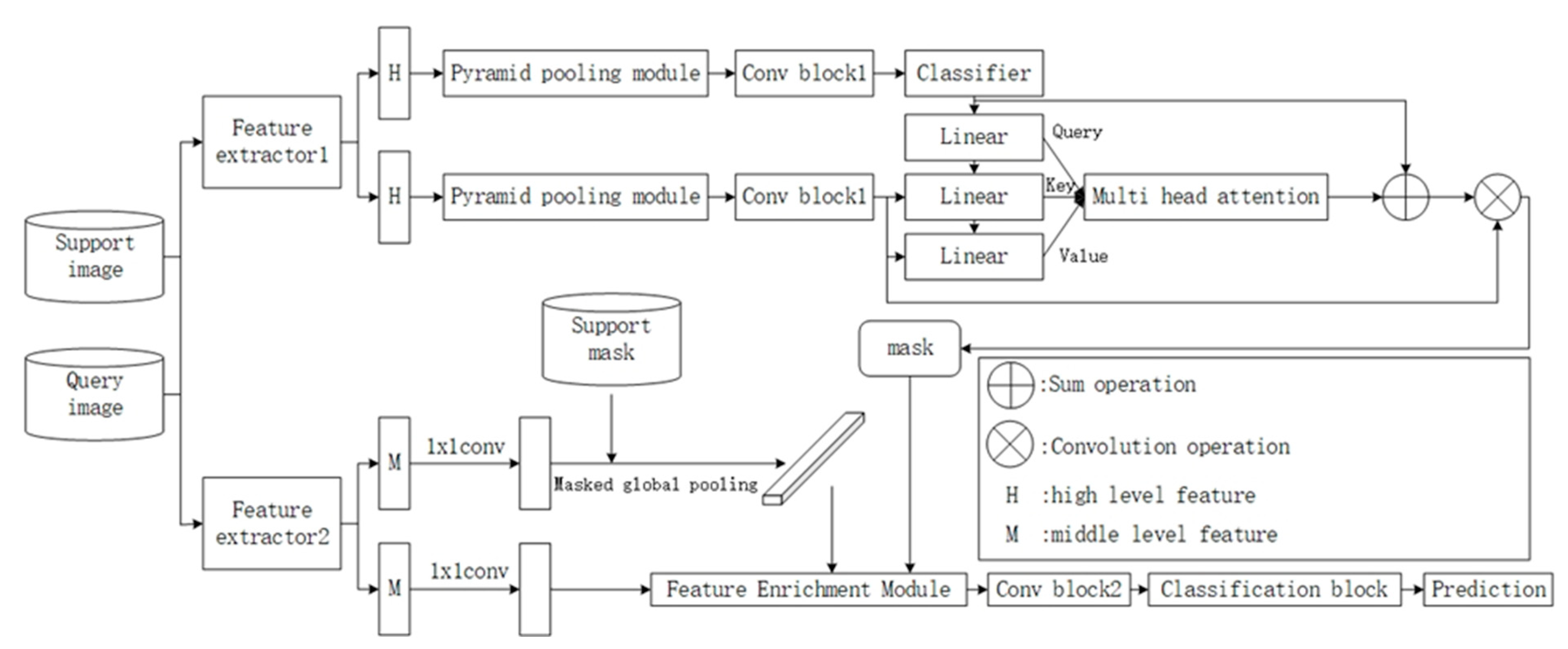
4.1.2. Meta-Learning Classification Weight Transfer Network for Generating Masked Few-Shot Image Segmentation Framework

The second experimental architecture proposed in this paper is the primary experimental framework, which is an improvement upon the CWT architecture proposed by Lu, Z. et al. [33] and the PFENet architecture proposed by Zhuotao Tian et al. [34]. The motivation for this improvement is inspired by the approach of PFENet++ [35], an evolved version of PFENet. PFENet++ improves upon PFENet by modifying the method of generating prior masks, shifting from a non-training approach to a training-based approach for generating prior masks containing contextual feature information, leading to better overall model performance. Therefore, in the design of the second experimental architecture, this paper adopts the CWT method to generate prior masks with higher accuracy and combines it with the PFENet approach to design the overall experimental framework. The experimental architecture flowchart is shown in Figure 4. Feature extractors 1 and 2, the Pyramid Pooling Module, Conv Block1, and the settings of the first experimental architecture are the same, so they will be introduced in Section 4.2. Section 4.3 will discuss the classifier weight transformer (CWT), Section 4.4 will introduce the method of prior mask generation, and the Feature Enrichment Module (FEM), Conv Block2, and classification block will be discussed in Section 4.5.
Algorithm 5 is the steps for experimental training and testing:
Algorithm 5. Meta-Training
Require: D(T): 60 classes’ data for meta-training
Require: CVT: pre-trained classifier weight transformer
 1: for all epoch:
 2:  Sample support image and query image from D(T)
 3:  Extract support feature by feature extractor 1 and Pyramid Pooling Module
 4:  for i in range (200)
 5:   Use support feature training the classifier
 6:  end for
 7:  Extract query feature by feature extractor 1 and Pyramid Pooling Module
 8:  Calculate the new query weights by CWT and generate query mask
 9:  Extract support and query middle-level feature M
 10:  Input M and query mask to Feature Enrichment Module, then get new query feature
 11:  Predict the result by classification block
 12:  Compute the loss
 13:  Update Feature Enrichment Module, Conv Block2, classification block parameters
 14: end for
  • The dataset used in this experiment consists of a total of 80 classes, which will be divided into four branches, each containing 20 classes. During training, 60 of these classes will be utilized. The query image serves as the segmentation target.
  • In Figure 4, both feature extractor 1, Pyramid Pooling Module, Conv Block1, linear, and feature extractor 2 utilize pre-trained parameters. These parameters remain unchanged during both the training and testing phases.
  • Taking the five-shot experiment as an example, five annotated images per class are randomly sampled from the training data to serve as support images, while one annotated image per class is designated as the query image. Subsequently, feature extractor 1 and feature extractor 2 are employed to individually extract high-order features (H) and mid-order features (M).
  • Next, in Figure 4, utilizing the high-order features from the support images, a linear classifier is trained. The high-order features extracted from the query image are inputted into the pre-trained linear layer to compute the attention score for the query. This score is then convolved with the query features to generate a mask.
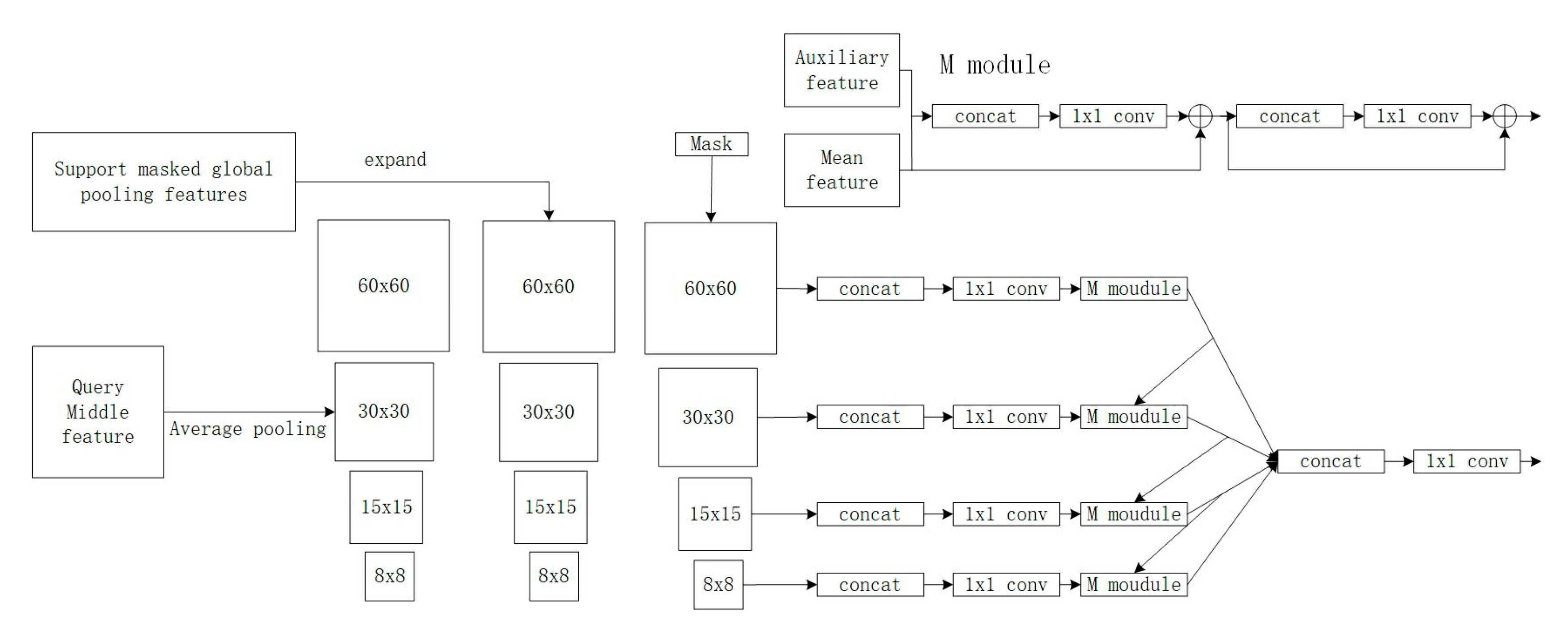
  • Following this, the mid-order features (M) extracted from both the support and query images, along with the mask generated in steps 3 and 4, are inputted into the Feature Enrichment Module (FEM). This process generates new query features, which are then passed through Conv Block2 and the classification block to predict the final results and update the parameters of the Feature Enrichment Module, Conv Block2, and classification block.
Algorithm 6 is the steps for experimental training and testing:
Algorithm 6. Meta-Testing
Require: D(T): 20 classes’ data for meta-testing
Require: CWT: pre-trained classifier weight transformer
Require: FEM: meta-trained Feature Enrichment Module
 1: for all epochs:
 2:  Sample support image and query image from D(T)
 3:  Extract support feature by feature extractor 1 and pyramid pooling module
 4:  for i in range (200)
 5:   Use support feature training the classifier
 6:  end for
 7:  Extract query feature by feature extractor 1 and pyramid pooling module
 8:  Calculate the new query weights by CWT and generate query mask
 9:  Extract support and query middle-level feature M by feature extractor 2
10:  Input M and query mask to FEM, then get new query feature
11:  Predict the result by trained classification block
12: end for
  • For the test phase, the remaining 20 classes are utilized, with five annotated images randomly sampled per class to serve as support images, along with one unlabeled query image.
  • The method of generating the mask follows the same procedure as steps 3–4 during training. Subsequently, the mask, mid-order features of the query image, and mid-order features of the support images are inputted into the trained Feature Enrichment Module, conv block2, and classification block to predict the results for the query image.

4.2. Feature Extraction

This section will introduce the feature extraction method and the Pyramid Pooling Module (PPM) used in this paper.
Both experimental architectures in the paper utilize the ResNet-50V2 [36] architecture for the feature extractor. As depicted in Figure 5, the number of residual blocks per layer, as well as the sizes and channel numbers of convolutional layers, are listed in Table 1. The structure of residual blocks is shown in Figure 6. In the first experimental architecture, image features are extracted from the complete ResNet-50V2, specifically from Layer 4 as shown in Figure 5, and then inputted into the Pyramid Pooling Module. In the second experimental architecture, high-level features are also extracted from Layer 4, while mid-level features are concatenated from features extracted from Layer 2 and Layer 3.
In the experimental architecture, mid-level and high-level features are set according to the method used in PFENet, as its improved version PFENet++ also utilizes mid-level and high-level features for experimental design. It solely employs high-level features to generate contextual information and relevance masks, which are then used for subsequent feature extraction with mid-level features, thus improving the overall model performance. Moreover, in the CWT method, high-level features are also used for result prediction. Therefore, the second experimental architecture in the paper adopts settings similar to those of the original PFENet.
In the first experimental architecture, the feature extractor uses pre-trained parameters from the training classes. However, in the second experimental architecture, feature extractor 1, like the feature extraction in the first architecture, uses parameters pre-trained with the training classes, while feature extractor 2 utilizes pre-training parameters from ImageNet.
Next, let us introduce the Pyramid Pooling Module (PPM) [27], whose architecture is illustrated in Figure 7. It takes high-level features extracted by ResNet-50V2 as input and utilizes four different pooling sizes to extract features of various scales. This approach enables the model to capture more global information compared to a single pooling operation, thus preserving features with global contextual information. In this paper, the pyramid pooling sizes used are 1 × 1, 2 × 2, 3 × 3, and 6 × 6 pooling. Figure 8 represents Conv Block1, which takes the features extracted by the pyramid pooling module as input and outputs them to the classifier for classification.
In both the first and second experimental architectures, the Pyramid Pooling Module and Conv Block1 are initially trained with pre-trained parameters for feature extraction. However, in the first experimental architecture, the support image updates the Pyramid Pooling Module and Conv Block1, while in the second experimental architecture, they remain unchanged.
The Pyramid Pooling Module in the second experimental architecture is designed following the methodology of the original CWT (baseline1). In the CWT approach, both the pyramid pooling module and feature extractor utilize pre-trained parameters for feature extraction, resulting in good segmentation results. In the subsequent second experimental architecture, generating a mask with higher accuracy proves beneficial for model performance. Therefore, the design of pooling sizes in the second experimental architecture follows the same approach as in the original CWT and also employs pre-trained parameters. Thus, in the second experimental architecture, the CWT for generating query masks maintains the settings of the original CWT method.

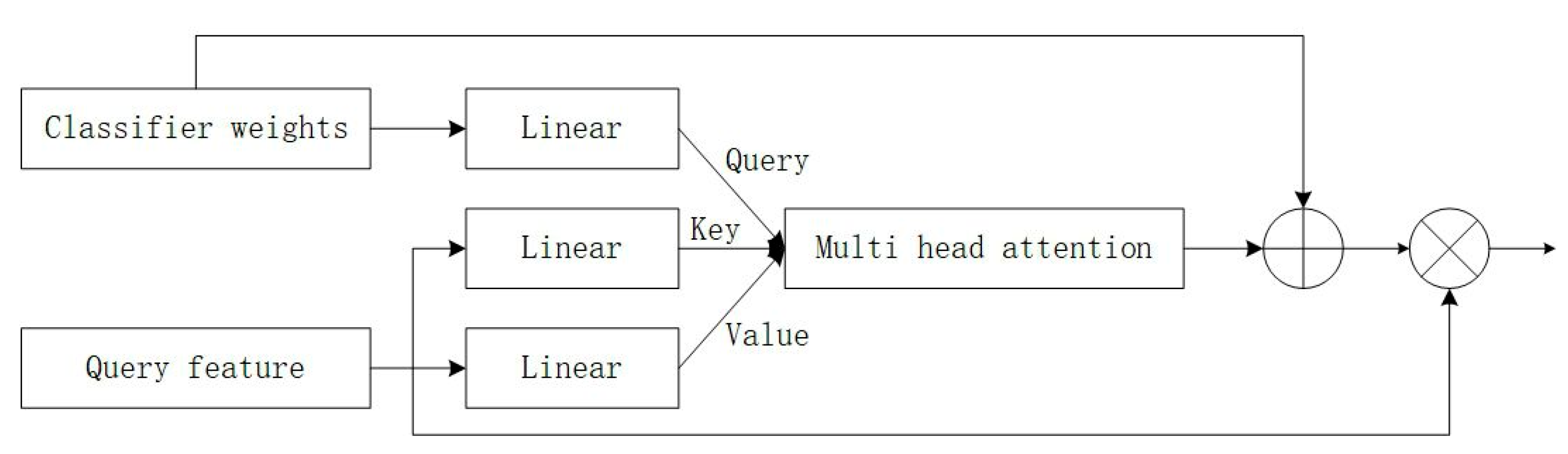
4.3. Classifier Weight Transformer

Next, let us introduce the Classifier Weight Transformer (CWT) [33]. Its inputs are the parameters of the classifier trained with the support image and the features extracted from the query image by the Pyramid Pooling Module and Conv Block1. The expressions (4) and (5) illustrate this. Here, w represents the parameters of the classifier trained with the support image, and F q represents the features extracted from the query image through the Pyramid Pooling Module. W q , W k , W v are learnable coefficients, while Ψ denotes a linear layer. The flow diagram is shown in Figure 9. This process allows the classifier trained with the support image to adapt to each query image.
In the second experimental architecture described in this paper, for the method that generates the mask, only the parameters of the classifier are updated, without making any updates to other parts of the CWT’s network architecture.
Q u e r y = w W q , K e y = F q W k , V a l u e = F q W v
w = w + Ψ s o f t m a x w W q F q W k T d a F q W v

4.4. Prior Mask Generation

In the second experimental architecture, the generation of the blue mask as depicted in Figure 4 follows the approach proposed by Lu, Z. et al. utilizing the CWT architecture. First, I utilize meta-learning to train a Classifier Weight Transformer (CWT) on 60 classes during training. The feature extractor 1, Pyramid Pooling Module, and Conv Block1 all utilize previously trained network parameters pre-trained on the 60 classes as described in Section 4.2. Then, the trained CWT is used to generate the mask inputted into the Feature Enrichment Module. The generation steps are as follows:
  • Input the high-level features of the support image, extract contextual information through the Pyramid Pooling Module, and train a temporary classifier.
  • Input the high-level features of the query image through the Pyramid Pooling Module, and use the trained Classifier Weight Transformer (CWT) to predict the mask.
In the second experimental architecture, the mask generation method is equivalent to performing meta-testing for the Classifier Weight Transformer.

4.5. Feature Enhancement

This subsection introduces the Feature Enrichment Module (FEM), as well as the subsequent Conv Block2 and classification block used in the second experimental architecture. The Feature Enrichment Module, depicted in Figure 10, takes intermediate features extracted from the query image and performs average pooling to obtain four different sizes of features: {60 × 60, 30 × 30, 15 × 15, 8 × 8}. Then, it multiplies the intermediate features extracted from the support image by the support mask, performs average pooling, and expands the resulting features to the size of {60 × 60, 30 × 30, 15 × 15, 8 × 8}. Next, the mask generated in Section 4.4 is resized to the same four different sizes mentioned above. The features and masks of the same size are concatenated together and processed by 1 × 1 convolutions to reduce the channel size to 256. They are then inputted into the Merge Module (M module), where the size of the auxiliary features is adjusted to match that of the main features. Subsequently, concatenation is used to combine the main features with the auxiliary features, and 1 × 1 convolutions are applied to extract information between the two features. The original main features are added, and two 3 × 3 convolutions are used for feature extraction, resulting in refined features. The residual connection in the Merge Module aims to preserve the integrity of the main features in the output. In Figure 10, for the 60 × 60-sized features inputted into the Merge Module, there are no auxiliary features; only the main features undergo two 3 × 3 convolutions and residual connection. Finally, the four different sizes of features generated by the Merge Module are concatenated, and after reducing the channel size with 1 × 1 convolutions, they are outputted to Conv Block2 in Figure 11 and then inputted into the classification block in Figure 12 for classification and outputting prediction results.
In the Feature Enrichment Module, this top-down pathway enables the integration of information from finer features to coarser features, facilitating the establishment of contextual relationships and overall performance improvement.

4.6. Loss Function

This subsection introduces the loss functions utilized in the experiments conducted in this paper. Cross-entropy (CE) [37] is employed as the loss function in both experimental architectures, as follows:
L C E = i = 1 C y i l o g p i
where:
-
C is the number of classes. Since our target is to segment the foreground and background, C = 2.
-
y i represents the ground truth labels of the target image
-
p i denotes the predicted results.
The loss function for the second experimental architecture is illustrated in Equation (7). Here, L C E 1 i , i 1,2 , 3,4 signifies the intermediate supervised losses, computed for the features outputted by the Merge Module in the Feature Enrichment Module. L C E 2 represents the loss for the final predicted results, where σ is the weight balancing the intermediate supervision, set to 1 in the experiments.
L = σ n i = 1 n L C E 1 i + L C E 2

5. Experimental Results and Analysis

This section presents a comparison and analysis of the experimental results of the proposed meta-learning model for few-shot image segmentation. It will discuss the experimental setup, including the environment and parameters, describe the datasets and evaluation metrics used, and finally, compare and analyze the experimental results with the modified experimental architectures.

5.1. Experimental Environment and Setup

The experiments in this paper were conducted on an Ubuntu 18.04 operating system, utilizing an Intel Core i7-9700k @ 3.60GHz processor (CPU) and a GeForce RTX2080 8 GB graphics adapter (GPU) to accelerate deep learning computations. The coding part was done using the widely used open-source Python machine learning library, PyTorch. Table 2 is the Specifications of Experimental Hardware and Training Parameters
For model training parameters, a total of 15 epochs were used, employing the Stochastic Gradient Descent (SGD) optimizer for parameter updates during backpropagation. The initial learning rate was set to 0.0025, with a decrease of 0.0001 for every iteration to aid convergence. The input image size was set to 473 × 473.

5.2. Experimental Dataset

The COCO- 20 i dataset [38,39] was utilized in this paper, which is currently the largest and most challenging dataset in the few-shot segmentation domain. It provides both train and validation sets, totaling 82,081/40,137 images, with the same 80 categories in both sets, selected from the COCO dataset [38]. Then, based on [39], the 80 classes in COCO- 20 i were divided into 4 branches denoted by i∈{0,1,2,3}, with each branch containing 20 categories. The detailed class distribution is shown in Table 3.
In a single experiment, three branches are used as meta-training data, while the remaining 1 branch serves as meta-testing data. Thus, 60 classes from the train set are used for meta-training, and 20 classes from the validation set are used for meta-testing. For instance, split-0, split-1, and split-2 from the train set are used for meta-training, while split-3 from the validation set is used for meta-testing.

5.3. Evaluation Mechanism

As for the evaluation mechanism used for image segmentation in this paper, it employs the mean Intersection over Union (mIOU) [40], which is a semantic segmentation metric measuring the degree of segmentation for images. It calculates the Mean Intersection over Union of two sets, namely the model’s predicted results and the ground truth annotations.
The formula for mean Intersection over Union (mIOU) is as follows:
I O U = T P T P + F P + F N
m I O U = 1 C i = 1 C I O U i
Equation (9) in this paper represents the class-wise mean Intersection over Union, which is the sum of the intersection over union for each class divided by the total number of classes C.
Equation (8) presents another form of intersection over union calculation, which computes the overlapping region of the image target and prediction divided by their union. Here, TP, FN, and FP are defined as follows:
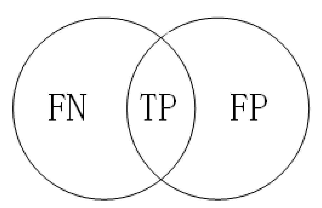
  • TP (True Positive): Pixels labeled as 1 in the ground truth and predicted as 1 by the model, or pixels labeled as 0 in the ground truth and predicted as 0, indicating correct predictions.
  • FN (False Negative): Pixels labeled as 0 in the ground truth but predicted as 1 by the model, representing prediction errors.
  • FP (False Positive): Pixels labeled as 1 in the ground truth but predicted as 0 by the model, indicating prediction errors.
Figure 13 can help us understand more quickly how Equations (8) and (9) evaluate the model’s prediction performance.
In model evaluation, four experiments are conducted, and the average intersection over union (IoU) of each experiment is taken as the final model performance. For example, if split-3 of the validation set is chosen as the target categories for meta-testing, split-0, split-1, and split-2 from the training set are used as meta-training categories, and so on. Each split-0, split-1, and split-2 is used as meta-testing categories, and the average results are obtained by averaging across all branches. Furthermore, the experiments are conducted using both one-shot and five-shot settings. In one-shot, only one annotated image is used as the support image during meta-testing, while the segmentation target (query image) is an unannotated image. In five-shot, five annotated images are used as support images during meta-testing, while the segmentation target (query image) remains unannotated.

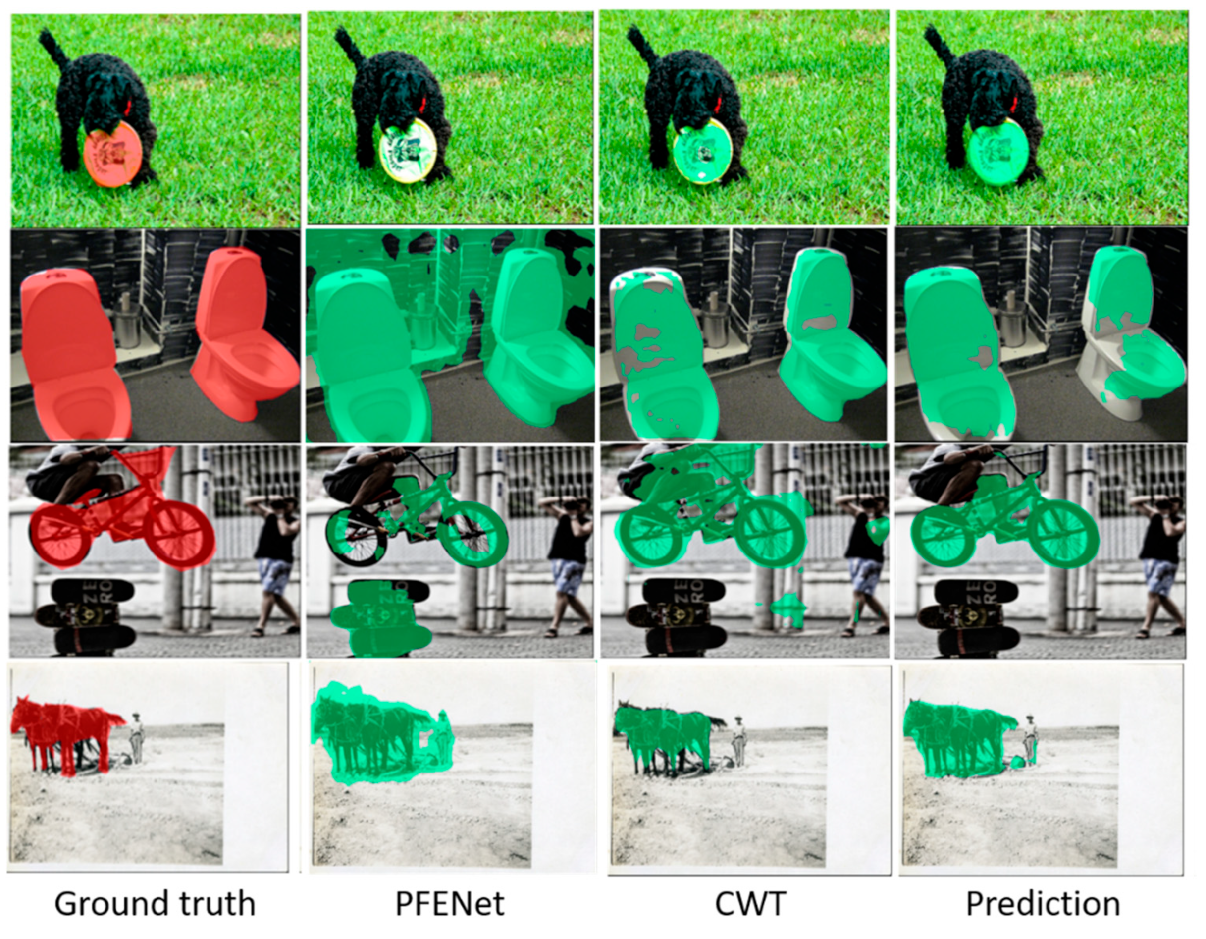
5.4. Experimental Results Comparison and Analysis

In this section, the performance of the proposed unified mean Intersection over Union (mIOU) mechanism is evaluated using the COCO- 20 i evaluation dataset (validation set) to assess model performance. Firstly, the evaluation of the first experimental architecture will be compared with CWT, as the first experimental architecture is derived from improvements made to CWT. Additionally, the second experimental architecture proposed, “Generating Masked Few-Shot Image Segmentation with Meta-Learning Weight Transfer Networks”, is based on improvements to the architectures of PFENet and CWT, hence it will be compared with PFENet and CWT. Moreover, considering the improvements are inspired by PFENet++, comparisons will also include PFENet++.
  • Experimental Architecture 1: Updated Partial Network CWT Architecture
    One-shot Experiment: As shown in Table 4, where mIOU is converted to percentages (%) for comparison.
Table 4. Experimental Results of Updated Partial Network CWT in One-shot Experiment.
MethodsSplit-0Split-1Split-2Split-3Mean
CWT32.236.031.631.632.9
PFENet34.333.032.330.132.4
PFENet++40.946.042.340.142.3
Proposed 28.035.734.338.434.1
As seen in Table 4, for the proposed first experimental architecture where partial network updates of CWT are employed, the average joint mean Intersection over Union of the four branches in the one-shot experiment is 2% higher than the original CWT architecture. Although the performance in split-0 and split-1 is lower than the baseline CWT architecture, overall model performance is improved compared to CWT. This indicates that training multiple pyramid pooling modules and convolutional layers during meta-training and meta-testing stages is somewhat beneficial for subsequent target image segmentation.
5-shot Experiment: As shown in Table 5, where mIOU is converted to percentages (%) for comparison.
As shown in Table 5, for the proposed first experimental architecture, which involves updating parts of the CWT network, the average joint mean Intersection over Union of the four branches in the five-shot experiment is 2.3% lower than the original CWT architecture. The performance in split-0 and split-1 is similar to the one-shot results, all of which are lower than the baseline CWT architecture. Hence, this architecture proposed in the first experiment performs relatively poorly in learning for split-0 and split-1. Additionally, its performance is relatively poor in handling a larger number of samples (five-shot). Based on the results from Table 4 and Table 5, the first proposed experimental architecture, involving updating parts of the CWT network, does not lead to a significant improvement in the overall model performance; at most, it can only maintain the experimental results obtained from training the original model.
Next, we present the results of the second experimental architecture proposed in this paper: a meta-learning classification weight transfer network to generate masking for few-shot image segmentation.
  • Experimental Architecture 2: Meta-learning Classification Weight Transfer Network for Generating Masks in Few-shot Image Segmentation
This experiment is the primary experimental architecture proposed in this paper for few-shot image segmentation using meta-learning, mainly utilizing a classification weight transfer network to generate effective prior masking to train an outstanding few-shot image segmentation network.
The reason for not following the design of the first experiment when conducting the second experiment is that in the first experiment, training the model with multiple updates to the pyramid pooling module in feature extraction would consume twice the training time compared to the original CWT method, and the model’s performance was not as good as the original CWT method. In the second experiment, CWT was used to generate better query masks. If the first experimental design were followed, because more parameters would need to be updated, the training time of the model would increase by 2 to 3 times. Therefore, the first experimental design was not chosen for the second experiment. Thus, in the following experiments, the method proposed in this paper for generating masks is the same as the original setting of CWT. Similar to PFENet++, the second experimental architecture proposed in this paper only changes the method of mask generation.
The following experiments analyze and compare the results of one-shot and five-shot experiments.
One-shot Experiment: As shown in Table 6, where mIOU is converted to percentages (%) for comparison.
As shown in Table 6, in the experimental architecture proposed in this paper, when employing superior prior masking, the model’s performance in one-shot scenarios across split-0, split-1, and split-3 demonstrates segmentation performance better than the original baseline, with split-2 also exhibiting similar performance to the baseline. In terms of the overall model performance across the four branches, the architecture proposed in this paper shows an improvement of 1.7% to 2.2% compared to the baseline.
  • Five-shot Experiment: As shown in Table 7, where mIOU is converted to percentages (%) for comparison.
Table 7. The results of 5-shot experiments on few-shot image segmentation using meta-learning for class-weight transfer network-generated masks.
MethodsSplit-0Split-1Split-2Split-3Mean
CWT40.143.839.042.441.3
PFENet38.538.638.234.337.4
PFENet++47.553.347.346.448.6
Proposed42.947.040.245.843.9
Table 7 summarizes the performance of our second proposed architecture, which utilizes meta-learning to transfer class weights to network-generated masks within a five-shot few-shot image segmentation framework. This approach, where the PFENet model leverages superior masks generated by the weight classifier transfer, outperforms the baseline model in all four branches of the five-shot experiment. The improvement in overall segmentation accuracy ranges from 2.6% to 6.5%. While our proposed architecture achieves lower performance compared to PFENet++ in both one-shot and five-shot settings, it demonstrates synergy when combined with CWT and PFENet. This combination surpasses the performance of the original baselines. These results suggest that incorporating CWT for mask generation, as proposed in this paper, is an effective way to improve the overall performance of PFENet, even if it doesn’t outperform PFENet++ alone.
The following Figure 14, Figure 15, Figure 16, Figure 17, Figure 18, Figure 19, Figure 20 and Figure 21 visualize the test results of few-shot image segmentation with meta-learning for class-weight transfer network-generated masks, including images segmented by each branch in the one-shot experiment and the five-shot experiment.
In the second experimental architecture, middle-level features are incorporated to generate masks.
In this paper, our choice of using only high-level features for mask generation is motivated by two factors:
-
Consistency with CWT: The original CWT method, which also employs high-level features for feature extraction and segmentation, achieved the best performance in their experiments. Maintaining consistency with this approach simplifies the comparison.
-
Alignment with PFENet++ Improvements: Recent advancements in PFENet++, particularly its use of high-level features to generate masks with contextual information, have shown positive impacts on overall model performance. This suggests that focusing on high-level features can be beneficial.
To explore the potential benefits of incorporating middle-level features, we conducted further experiments. Table 8 and Table 9 present the results when middle-level features are included during mask generation in the CWT framework. Table 8 shows the performance in the one-shot setting, while Table 9 focuses on the five-shot experiments.
From the experimental results, it can be observed that incorporating middle-level features into mask generation does not improve the model performance. Therefore, according to the experimental design, sticking to the original baseline setting would yield the best results.

6. Conclusions and Future Outlook

This paper proposes a novel technique for generating masks in few-shot image segmentation using a meta-learning classification weight transfer network. It employs a distinct method for prior mask generation, leveraging the architecture of a pre-trained meta-learning classification weight transferor to produce high-accuracy masks for query images based on the high-order features of query and support images. Subsequently, an input Feature Enrichment Module gathers information between feature maps of different sizes, ultimately generating new feature maps for the query image for segmentation. The experimental results demonstrate that utilizing the meta-learning classification weight transfer network to generate masks enhances the training effectiveness for few-shot image segmentation of new classes. Evaluated by the mean Intersection over Union (mIOU) metric, compared to the baseline, the overall mIOU increases by 1.7% in one-shot experiments and by 2.6% in five-shot experiments. However, there remains a gap between the performance of the proposed method and the state-of-the-art PFENet++. Drawing inspiration from the improvement techniques of PFENet++, we designed the experimental architecture of this paper. It is evident that generating effective prior masks contributes to improving model performance. Therefore, in future research, exploring various methods for generating prior masks could further enhance model performance.
The proposed meta-learning few-shot image segmentation model exhibits decent segmentation accuracy compared to the baseline. While it falls short of the state-of-the-art methods, it demonstrates a fundamental performance for segmenting images of new classes with few samples. However, the current study focuses on training and testing on the COCO- 20 i dataset, which presents a challenging dataset compared to others. Considering real-world applications, the accuracy of the experimental architecture has not yet reached practical application levels. Furthermore, the statistical characteristics of datasets collected using different devices vary, thereby influencing the model’s performance on datasets of new classes with different statistical distributions. Hence, there is significant room for improvement in the proposed method to address these issues. In future research, we aim to enhance the accuracy of this technique and enable it to handle few-shot image segmentation of new classes across datasets with different statistical distributions, thereby facilitating its practical application in real life.

Author Contributions

Conceptualization, J.-C.W. and P.-C.C.; Methodology, F.-C.J. and C.-Y.W.; writing—original draft preparation, F.-C.J.; writing—review and editing, J.-H.W., P.T.L., M.-H.S., K.-C.L., S.-L.C., T.P. and J.-L.H.; supervision, P.-C.C. All authors have read and agreed to the published version of the manuscript.

Funding

This research received no external funding.

Institutional Review Board Statement

Not applicable.

Informed Consent Statement

Not applicable.

Data Availability Statement

Data are contained within the article.

Conflicts of Interest

The authors declare no conflicts of interest.

Appendix A

Figure A1. Self-Attention Diagram.
Electronics 13 02634 g0a1
Figure A2. Multi Head Self Attention Diagram.
Electronics 13 02634 g0a2

References

  1. Vu, D.-Q.; Le, N.; Wang, J.-C. Teaching Yourself: A Self-Knowledge Distillation Approach to Action Recognition. IEEE Access 2021, 9, 105711–105723. [Google Scholar] [CrossRef]
  2. Cao, H.N.; Duc-Quang, V.; Huong, H.L.; Chien-Lin, H.; Jia-Ching, W. Cyclic Transfer Learning for Mandarin-English Code-Switching Speech Recognition. IEEE Signal Process. Lett. 2023, 30, 1387–1391. [Google Scholar]
  3. Pranata, Y.D.; Wang, K.-C.; Wang, J.-C.; Idram, I.; Lai, J.-Y.; Liu, J.-W.; Hsieh, I.-H. Deep Learning and SURF for Automated Classification and Detection of Calcaneus Fractures in CT Images. Comput. Methods Programs Biomed. 2019, 171, 27–37. [Google Scholar] [CrossRef] [PubMed]
  4. Thi Le, P.; Pham, T.; Hsu, Y.-C.; Wang, J.-C. Convolutional Blur Attention Network for Cell Nuclei Segmentation. Sensors 2022, 22, 1586. [Google Scholar] [CrossRef] [PubMed]
  5. Putri, W.R.; Liu, S.-H.; Aslam, M.S.; Li, Y.-H.; Chang, C.-C.; Wang, J.-C. Self-Supervised Learning Framework toward State-of-the-Art Iris Image Segmentation. Sensors 2022, 22, 2133. [Google Scholar] [CrossRef] [PubMed]
  6. Wang, C.-Y.; Chang, P.-C.; Ding, J.-J.; Tai, T.-C.; Santoso, A.; Liu, Y.-T.; Wang, J.-C. Spectral–Temporal Receptive Field-Based Descriptors and Hierarchical Cascade Deep Belief Network for Guitar Playing Technique Classification. IEEE Trans. Cybern. 2022, 52, 3684–3695. [Google Scholar] [CrossRef]
  7. Wang, C.-Y.; Tai, T.-C.; Wang, J.-C.; Santoso, A.; Mathulaprangsan, S.; Chiang, C.-C.; Wu, C.-H. Sound Events Recognition and Retrieval Using Multi-Convolutional-Channel Sparse Coding Convolutional Neural Networks. IEEE/ACM Trans. Audio Speech Lang. Process. 2020, 28, 1875–1887. [Google Scholar] [CrossRef]
  8. Quintero, F.O.L.; Contreras-Reyes, J.E. Estimation for finite mixture of simplex models: Applications to biomedical data. Stat. Model. 2018, 18, 129–148. [Google Scholar] [CrossRef]
  9. Ranaldi, L.; Pucci, G. Knowing Knowledge: Epistemological Study of Knowledge in Transformers. Appl. Sci. 2023, 13, 677. [Google Scholar] [CrossRef]
  10. Wang, K.; Wang, X.; Cheng, Y. Few-shot learning based on enhanced pseudo-labels and graded pseudo-labeled data selection. Int. J. Mach. Learn. Cybern. 2023, 14, 1783–1795. [Google Scholar] [CrossRef]
  11. Jiang, C.; Wang, T.; Li, S.; Wang, J.; Wang, S.; Antoniou, A. Few-shot Class-Incremental Semantic Segmentation via Pseudo-Labeling and Knowledge Distillation. In Proceedings of the 2023 4th International Conference on Information Science, Parallel and Distributed Systems (ISPDS), Guangzhou, China, 14–16 July 2023; IEEE: Piscataway, NJ, USA, 2023. [Google Scholar]
  12. Yu, X.; Ouyang, B.; Principe, J.C.; Farrington, S.; Reed, J.; Li, Y. Weakly supervised learning of point-level annotation for coral image segmentation. In Proceedings of the OCEANS 2019 MTS/IEEE SEATTLE, Seattle, WA, USA, 27–31 October 2019; IEEE: Piscataway, NJ, USA, 2019; pp. 1–7. [Google Scholar]
  13. Jhou, F.-C.; Liang, K.-W.; Lo, C.-H.; Wang, C.-Y.; Chen, Y.-F.; Wang, J.-C.; Chang, P.-C. Mask Generation with Meta-Learning Classifier Weight Transformer Network for Few-Shot Image Segmentation. In Proceedings of the 2023 International Conference on Consumer Electronics—Taiwan (ICCE-Taiwan), PingTung, Taiwan, 17–19 July 2023; pp. 457–458. [Google Scholar]
  14. Bahdanau, D.; Cho, K.; Bengio, Y. Neural Machine Translation by Jointly Learning to Align and Translate. arXiv 2014, arXiv:1409.0473. [Google Scholar]
  15. Vaswani, A.; Shazeer, N.; Parmar, N.; Uszkoreit, J.; Jones, L.; Gomez, A.N.; Kaiser, L.; Polosukhin, I. Attention Is All You Need. Neural Inf. Process. Syst. 2017, 30. [Google Scholar]
  16. Finn, C.; Abbeel, P.; Levine, S. Model-Agnostic Meta-Learning for Fast Adaptation of Deep Networks. Proc. Mach. Learn. Res. 2017, 70, 1126–1135. [Google Scholar]
  17. Snell, J.; Swersky, K.; Zemel, R. Prototypical Networks for Few-Shot Learning. Neural Inf. Process. Syst. 2017, 30. [Google Scholar]
  18. Gidaris, S.; Komodakis, N. Dynamic Few-Shot Visual Learning without Forgetting. In Proceedings of the 2018 IEEE/CVF Conference on Computer Vision and Pattern Recognition, Salt Lake City, UT, USA, 18–23 June 2018. [Google Scholar]
  19. Goldblum, M.; Reich, S.; Fowl, L.; Ni, R.; Cherepanova, V.; Goldstein, T. Unraveling Meta-Learning: Understanding Feature Representations for Few-Shot Tasks. Proc. Mach. Learn. Res. 2020, 119, 3607–3616. [Google Scholar]
  20. Liu, J.; Song, L.; Qin, Y. Prototype Rectification for Few-Shot Learning. In Proceedings of the Computer Vision—ECCV 2020, Lecture Notes in Computer Science, Glasgow, UK, 23–28 August 2020; pp. 741–756. [Google Scholar]
  21. Chen, Y.; Liu, Z.; Xu, H.; Darrell, T.; Wang, X. Meta-Baseline: Exploring Simple Meta-Learning for Few-Shot Learning. In Proceedings of the 2021 IEEE/CVF International Conference on Computer Vision (ICCV), Montreal, QC, Canada, 11–17 October 2021. [Google Scholar]
  22. Long, J.; Shelhamer, E.; Darrell, T. Fully Convolutional Networks for Semantic Segmentation. In Proceedings of the 2015 IEEE Conference on Computer Vision and Pattern Recognition (CVPR), Boston, MA, USA, 7–12 June 2015. [Google Scholar]
  23. Yu, F.; Koltun, V. Multi-Scale Context Aggregation by Dilated Convolutions. arXiv 2015, arXiv:1511.07122. [Google Scholar]
  24. Chen, L.-C.; Papandreou, G.; Kokkinos, I.; Murphy, K.; Yuille, A.L. DeepLab: Semantic Image Segmentation with Deep Convolutional Nets, Atrous Convolution, and Fully Connected CRFs. IEEE Trans. Pattern Anal. Mach. Intell. 2018, 40, 834–848. [Google Scholar] [CrossRef] [PubMed]
  25. Ronneberger, O.; Fischer, P.; Brox, T. U-Net: Convolutional Networks for Biomedical Image Segmentation. In Proceedings of the Lecture Notes in Computer Science, Medical Image Computing and Computer-Assisted Intervention—MICCAI 2015, Munich, Germany, 5–9 October 2015; pp. 234–241. [Google Scholar]
  26. Liu, W.; Rabinovich, A.; Berg, A.C. ParseNet: Looking Wider to See Better. arXiv 2015, arXiv:1506.04579. [Google Scholar]
  27. Zhao, H.; Shi, J.; Qi, X.; Wang, X.; Jia, J. Pyramid Scene Parsing Network. In Proceedings of the 2017 IEEE Conference on Computer Vision and Pattern Recognition (CVPR), Honolulu, HI, USA, 21–26 July 2017. [Google Scholar]
  28. Shaban, A.; Bansal, S.; Liu, Z.; Essa, I.; Boots, B. One-Shot Learning for Semantic Segmentation. In Proceedings of the British Machine Vision Conference 2017, London, UK, 4–7 September 2017. [Google Scholar]
  29. Dong, N.; Xing, E.P. Few-Shot Semantic Segmentation with Prototype Learning. In Proceedings of the British Machine Vision Conference 2018, Newcastle, UK, 3–6 September 2018. [Google Scholar]
  30. Wang, K.; Liew, J.H.; Zou, Y.; Zhou, D.; Feng, J. PANet: Few-Shot Image Semantic Segmentation with Prototype Alignment. In Proceedings of the 2019 IEEE/CVF International Conference on Computer Vision (ICCV), Seoul, Republic of Korea, 27 October–2 November 2019. [Google Scholar]
  31. Zhang, C.; Lin, G.; Liu, F.; Yao, R.; Shen, C. CANet: Class-Agnostic Segmentation Networks with Iterative Refinement and Attentive Few-Shot Learning. In Proceedings of the 2019 IEEE/CVF Conference on Computer Vision and Pattern Recognition (CVPR), Long Beach, CA, USA, 19–20 June 2019. [Google Scholar]
  32. Lin, G.; Milan, A.; Shen, C.; Reid, I. RefineNet: Multi-Path Refinement Networks for High-Resolution Semantic Segmentation. In Proceedings of the 2017 IEEE Conference on Computer Vision and Pattern Recognition (CVPR), Honolulu, HI, USA, 21–26 July 2017. [Google Scholar]
  33. Lu, Z.; He, S.; Zhu, X.; Zhang, L.; Song, Y.-Z.; Xiang, T. Simpler Is Better: Few-Shot Semantic Segmentation with Classifier Weight Transformer. In Proceedings of the 2021 IEEE/CVF International Conference on Computer Vision (ICCV), Montreal, BC, Canada, 11–17 October 2021. [Google Scholar]
  34. Tian, Z.; Zhao, H.; Shu, M.; Yang, Z.; Li, R.; Jia, J. Prior Guided Feature Enrichment Network for Few-Shot Segmentation. IEEE Trans. Pattern Anal. Mach. Intell. 2022, 44, 1050–1065. [Google Scholar] [CrossRef] [PubMed]
  35. Luo, X.; Tian, Z.; Zhang, T.; Yu, B.; Tang, Y.; Jia, J. PFENet++: Boosting Few-Shot Semantic Segmentation with the Noise-Filtered Context-Aware Prior Mask. arXiv 2021, arXiv:2109.13788. [Google Scholar] [CrossRef] [PubMed]
  36. He, K.; Zhang, X.; Ren, S.; Sun, J. Deep Residual Learning for Image Recognition. In Proceedings of the 2016 IEEE Conference on Computer Vision and Pattern Recognition (CVPR), Las Vegas, NV, USA, 27–30 June 2016; pp. 770–778. [Google Scholar]
  37. Ramírez-Parietti, I.; Contreras-Reyes, J.E.; Idrovo-Aguirre, B.J. Cross-sample entropy estimation for time series analysis: A nonparametric approach. Nonlinear Dyn. 2021, 105, 2485–2508. [Google Scholar] [CrossRef]
  38. Lin, T.-Y.; Maire, M.; Belongie, S.; Hays, J.; Perona, P.; Ramanan, D.; Dollár, P.; Zitnick, C.L. Microsoft COCO: Common Objects in Context. In Proceedings of the Computer Vision—ECCV 2014, Zurich, Switzerland, 6–12 September 2014; Lecture Notes in Computer Science. 2014; pp. 740–755. [Google Scholar]
  39. Nguyen, K.; Todorovic, S. Feature Weighting and Boosting for Few-Shot Segmentation. In Proceedings of the 2019 IEEE/CVF International Conference on Computer Vision (ICCV), Seoul, Republic of Korea, 27 October–2 November 2019. [Google Scholar]
  40. Semantic Segmentation Evaluation Index MIOU. Available online: https://blog.csdn.net/qq_34197944/article/details/103574436/ (accessed on 17 December 2019).
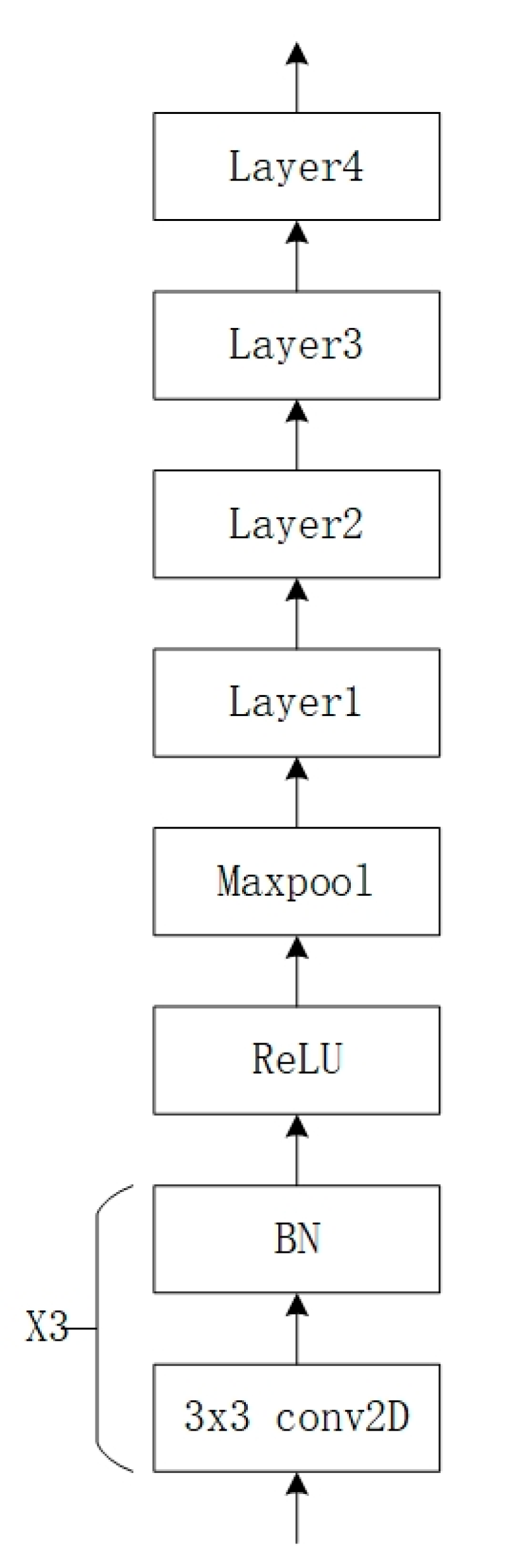
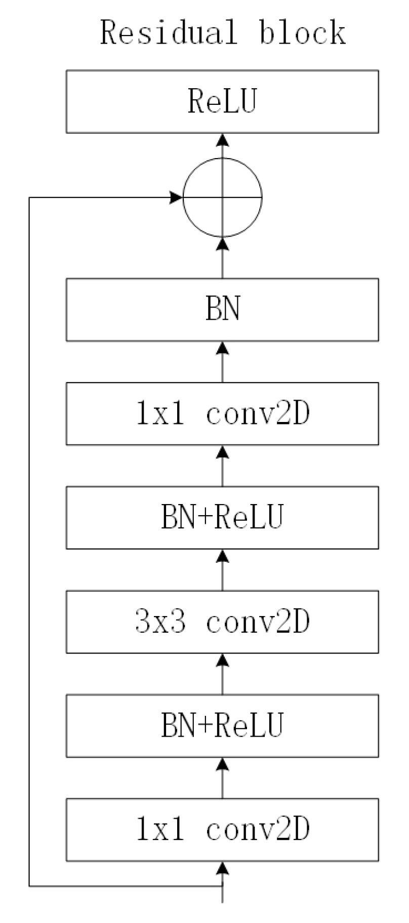
Figure 1. Illustration of Semantic Segmentation.
Electronics 13 02634 g001
Figure 2. Schematic diagram of image segmentation models combined with meta-learning.
Electronics 13 02634 g002
Figure 3. System Architecture Diagram 1.
Electronics 13 02634 g003
Figure 4. System Architecture Diagram 2.
Electronics 13 02634 g004
Figure 5. ResNet-50V2 Architecture Diagram.
Electronics 13 02634 g005
Figure 6. Residual Block Diagram.
Electronics 13 02634 g006
Figure 7. Pyramid pooling module.
Electronics 13 02634 g007
Figure 8. Conv Block1.
Electronics 13 02634 g008
Figure 9. Diagram of the Classifier Weight Transformer.
Electronics 13 02634 g009
Figure 10. Feature Enrichment Module.
Electronics 13 02634 g010
Figure 11. Conv Block2.
Electronics 13 02634 g011
Figure 12. Classification block.
Electronics 13 02634 g012
Figure 13. Model Prediction Evaluation Schematic.
Electronics 13 02634 g013
Figure 14. Visualization of one-shot split-0 image segmentation.
Electronics 13 02634 g014
Figure 15. Visualization of one-shot split-1 image segmentation.
Electronics 13 02634 g015
Figure 16. Visualization of one-shot split-2 image segmentation.
Electronics 13 02634 g016
Figure 17. Visualization of one-shot split-3 image segmentation.
Electronics 13 02634 g017
Figure 18. Visualization of five-shot split-0 image segmentation.
Electronics 13 02634 g018
Figure 19. Visualization of five-shot split-1 image segmentation.
Electronics 13 02634 g019
Figure 20. Visualization of five-shot split-2 image segmentation.
Electronics 13 02634 g020
Figure 21. Visualization of five-shot split-3 image segmentation.
Electronics 13 02634 g021
Table 1. Number of Residual Blocks in Each Layer of ResNet.
Layer NameResidual Blocks
Layer 1 1 × 1.64 3 × 3.64 1 × 1.256 × 3
Layer 2 1 × 1.128 3 × 3.128 1 × 1.512 × 4
Layer 3 1 × 1.256 3 × 3.256 1 × 1.1024 × 6
Layer 4 1 × 1.512 3 × 3.512 1 × 1.2048 × 3
Table 2. Specifications of Hardware and Training Parameters in the experiments.
DeviceParameters
CPUIntel Core i7-9700k @ 3.60 GHz
GPUGeForce RTX2080 8 GB
RAMDDR4-3200 MHz 64 GB
OSUbuntu 18.04
Software languagePython 3.7
Neural network toolPytorch
Training settingEpoch15
Classifier learning rate0.1
Learning rate0.0025
OptimizerSGD
Image size473 × 473
Table 3. Class Distribution of COCO- 20 i Branches.
Split-0Split-1Split-2Split-3
1: person2: bicycle3: car4: motorcycle
5: airplane6: bus7: train8: truck
9: boat10: traffic light11: fire hydrant12: stop sign
13: parking meter14: bench15: bird16: cat
17: dog18: horse19: sheep20: cow
21: elephant22: bear23: zebra24: giraffe
24: backpack26: umbrella27: handbag28: tie
29: suitcase30: frisbee31: skis32: snowboard
33: sports ball34: kite35: baseball bat36: baseball glove
37: skateboard38: surfboard39: tennis racket40: bottle
41: wine glass42: cup43: fork44: knife
45: spoon46: bowl47: banana48: apple
49: sandwich50: orange51: broccoli52: carrot
53: hot dog54: pizza55: donut56: cake
57: chair58: sofa59: potted plant60: bed
61: dining table62: toilet63: tv64: laptop
65: mouse66: remote67: keyboard68: cellphone
69: microwave70: oven71: toaster72: sink
73: refrigerator74: book75: clock76: vase
77: scissors78: teddy bear79: hair drier80: toothbrush
Table 5. Experimental Results of Updated Partial Network CWT in five-shot Experiment.
MethodsSplit-0Split-1Split-2Split-3Mean
CWT40.143.839.042.441.3
PFENet38.538.638.234.337.4
PFENet++47.553.347.346.448.6
Proposed 35.040.539.441.239.0
Table 6. Results of the one-shot experiment for the meta-learning classification weight transfer network to generate masking for few-shot image segmentation.
MethodsSplit-0Split-1Split-2Split-3Mean
CWT32.236.031.631.632.9
PFENet34.333.032.330.132.4
PFENet++40.946.042.340.142.3
Proposed 34.337.932.234.034.6
Table 8. One-shot results with middle-level features incorporated into mask generation.
MethodsSplit-0Split-1Split-2Split-3Mean
CWT32.236.031.631.632.9
PFENet34.333.032.330.132.4
PFENet++40.946.042.340.142.3
Proposed 34.337.932.234.034.6
Proposed
(H + M feature)
33.133.530.931.532.2
Table 9. Five-shot results with middle-level features incorporated into mask generation.
MethodsSplit-0Split-1Split-2Split-3Mean
CWT40.143.839.042.441.3
PFENet38.538.638.234.337.4
PFENet++47.553.347.346.448.6
Proposed42.947.040.245.843.9
Proposed
(H + M feature)
38.040.736.135.837.6
Disclaimer/Publisher’s Note: The statements, opinions and data contained in all publications are solely those of the individual author(s) and contributor(s) and not of MDPI and/or the editor(s). MDPI and/or the editor(s) disclaim responsibility for any injury to people or property resulting from any ideas, methods, instructions or products referred to in the content.

