Deep Residual-in-Residual Model-Based PET Image Super-Resolution with Motion Blur

Abstract

Positron emission tomography (PET) is a non-invasive molecular imaging technique. The limited spatial resolution of PET images, due to technological and physical imaging constraints, directly affects the precise localization and interpretation of small lesions and biological processes. The super-resolution (SR) technique aims to enhance image quality by improving spatial resolution, thereby aiding clinicians in achieving more accurate diagnoses. However, most conventional SR methods rely on idealized degradation models and fail to effectively capture both low- and high-frequency information present in medical images. For the challenging SR reconstruction of PET images exhibiting motion-induced artefacts, a degradation model that better aligns with practical scanning scenarios was designed by us. Furthermore, we proposed a PET image SR method based on the deep residual-in-residual network (DRRN), focusing on the recovery of both low- and high-frequency information. By incorporating multi-level residual connections, our approach facilitates direct feature propagation across different network levels. This design effectively mitigates the lack of feature correlation between adjacent convolutional layers in deep networks. Our proposed method surpasses benchmark methods in both full-reference and no-reference metrics and subjective visual effects across small animal PET (SAPET), phantoms, and Alzheimer’s Disease Neuroimaging Initiative (ADNI) datasets. The experimental findings confirm the remarkable efficacy of DRRN in enhancing spatial resolution and mitigating blurring in PET images. In comparison to conventional SR techniques, this method demonstrates superior proficiency in restoring low-frequency structural texture information while simultaneously maintaining high-frequency details, thus showcasing exceptional multi-frequency information fusion capabilities.

1. Introduction

PET plays an invaluable role in the realm of medical imaging, serving as a nuclear imaging technology with profound significance in both clinical applications and research [1]. It provides essential information on the body’s metabolic processes, and it is essential for the diagnosis of cancer and the evaluation of ailments, including heart disease and neurological disorders [2,3,4,5]. PET excels in discerning lesions from the surrounding healthy tissues due to its remarkable contrast capabilities. The limitations of PET imaging stem from a range of physical and technical factors, collectively affecting image resolution. Obtaining high-resolution (HR) PET images is hampered by factors such as motion blur, image reconstruction techniques, short scan periods, and detector scatter in addition to positron range, noncolinearity, and scatter [6]. The inherent physical limitations of PET result in a lower image resolution compared to MRI, CT, and X-ray modalities [7,8,9]. This poorer resolution leads to diffuse, blurred lesion boundaries, posing a significant challenge for accurate structure and lesion delineation, particularly in small regions of interest (ROIs) [10,11]. The intrinsic fuzziness and low resolution of PET images can greatly impact clinical decision-making, leading to erroneous lesion segmentation, missed diagnoses, and misdiagnoses. Improving PET hardware and software is essential to enhance image quality and diagnostic accuracy.

Within the field of medical imaging, advanced computer vision can enhance image quality [12], enable automatic lesion recognition and classification [13], and assist physicians in diagnosis. One promising application area of computer vision is image super-resolution (SR), which aims to reconstruct HR images from their low-resolution counterparts. As an affordable post-processing technology, SR can provide an alternative to the high cost of upgrading PET scanners to improve resolution. To advance the application of SR in the clinical domain [14], the focus should be on adapting SR methods to suit medical data nuances, demonstrating practical feasibility on a large scale. Through the comprehensive validation and continuous optimization of algorithms, SR will emerge as a key technology in the field of medical imaging. This technology holds great promise in providing physicians with high-quality diagnostic results under limited scanning settings.

Image super-resolution (SR) methods can be classified into three main categories: interpolation-based [15,16], reconstruction-based [17,18], and learning-based [19,20]. Interpolation methods, such as bilinear or bicubic interpolation, provide a straightforward approach in image processing. However, it is noted that these techniques often exhibit a tendency to emphasize smoothing characteristics, potentially resulting in the generation of blurred outputs, particularly when applied to complex images. Reconstruction-based methods can be further divided into frequency-domain and spatial-domain techniques, but they may struggle with generalization across diverse image types. In recent years, research focus in SR has shifted notably towards learning-based methodologies, particularly leveraging deep learning technologies. These methods involve training models with extensive datasets of high-resolution (HR) images, demonstrating superior representation capabilities compared to traditional techniques. In 2015, Dong et al. pioneered the application of convolutional neural networks to image SR, proposing a three-layer convolutional neural network for super-resolution (SRCNN) [21] that established an end-to-end mapping between HR and LR images. This end-to-end SR model utilizing a three-layer convolutional neural network requires no human intervention or multi-stage processing and achieved significant improvements in image reconstruction over traditional SR algorithms. Building upon the SRCNN [21] concept, researchers subsequently developed models such as the fast super-resolution convolutional neural network (FSRCNN) [22] and ESPCN [23]. However, the shallow network architectures of these models limit their ability to restore intricate features. To extract more feature maps and increase accuracy, Kim et al. [24] proposed the very deep super-resolution (VDSR) model, which expanded the original SRCNN’s depth. By learning the residual between HR and LR images, VDSR [24] attained higher fidelity results and faster training. Zhang et al. [25] further augmented network depth by introducing the very deep residual channel attention network (RCAN) for precision SR. Their residual-in-residual (RIR) structure enables the training of immensely deep networks focused on high-frequency details, while channel attention provides an adaptive scaling of features. Qiu et al. proposed an efficient medical image super-resolution (EMISR) [26] technique. EMISR integrates the SRCNN architecture with the sub-pixel convolution of the efficient sub-pixel convolutional neural network (ESPCN) [23], improving reconstruction accuracy and reducing processing time for knee MRI. Similarly, Song et al. [27] developed a CNN-based SR approach for PET, leveraging high-resolution MRI to facilitate resolution restoration. Encoding spatial input patch locations as additional CNN inputs accommodated the spatially varying fuzziness of PET nuclei. For retinal image SR, Qiu et al. [28] enhanced a generative adversarial network (GAN) algorithm with a novel residual attention block, improving high-frequency and texture detail. Zhu et al. [29] introduced a feedback attention network (FBAN) to address cardiac MRI SR, mitigating upsampling information loss and high-frequency reconstruction challenges.

Universally recognized, the SR problem is an inverse problem in which the unknown image is to be reconstructed based on the measurements associated with the additive noise through linear operators (geometric distortions, blurring, and extraction operations). Nowadays, most of the methods that have been proposed for SR are based on generic solutions of ordinary degradation, such as assuming a bicubic downsampling kernel without incorporating the actual degradation. While these methods can produce visually pleasing results, they often fail when applied to real images, particularly in medical imaging contexts. Existing SR techniques in medical imaging often rely on ideal scanning settings and ignore the challenges of physiological movement during the scanning process. In practical medical imaging scenarios, these methods encounter significant limitations due to inherent intricacies and real-world challenges. Conventional approaches utilizing generative adversarial networks (GANs) [30], convolutional neural networks (CNNs) [31], and attention networks [25] show promise in controlled settings but struggle with low-quality inputs affected by motion artifacts. The residual network for the SR of medical images proposed by Qiu et al. [32] and the SR attentional mechanism network for lung cancer images proposed by Zhu et al. [33] were degraded by Gaussian filtering in order to obtain an LR image. Gaussian filtering is a straightforward linear blurring technique that can only replicate the fundamental uniform blurring effect and ignores noise. A self-supervised SR (SSSR) method for PET based on CycleGAN was developed by Song et al. [34]. It does not account for noise and employs a spatially variant PSF in the degradation phase. The spatially variant PSF is usually used to characterize the non-uniform blurring of images at different locations without focusing more on physiological motion. These schemes can deal with a very limited number of blurred images, which may even be different from an actual measured image. In real scanning situations, due to the long duration of PET scanning, patients who have been on hold for a long period may experience irregular and complex physiological movements. However, even slight jerks may affect the image quality [35]. Therefore, it is particularly important to consider practical degradation issues in medical image SR tasks.

This study focuses on preclinical PET imaging, where mice were administered anesthetics to maintain stillness during scanning. Insufficient anesthetic can lead to substantial mouse movement, exacerbated by physiological twitching. In clinical PET imaging, patient discomfort may cause unconscious movements, resulting in uniform motion that can introduce artifacts, blurring, or distortion. To address these challenges, a deep residual-in-residual network (DRRN)-based SR approach for blurry PET images affected by pure translational motion and common space invariance was proposed by us, inspired by [36,37]. Motion blur point spread function (PSF) is applied in Wiener filtering to realistically replicate the micro-physiological motion blur induced by the scanned object in PET images. The main innovations of this paper can be briefly described as follows.

• The actual degradation due to physiological motion in a deep learning-based SR task for medical images is considered for the first time by us.
• A degradation model focusing on noise and simplified blur for the more complex SR recovery problem is designed by us. The directional motion blur present in the image is simulated to a certain degree using a motion blur PSF. Additionally, instead of a fixed K value of inverse signal-to-noise ratio (SNR) in the Wiener filtering, which lacks flexibility, K is implemented with variable parameters.
• In the reconstruction part, to address issues such as a loss of information during computation and potential degradation during the feature extraction process, a new network based on the deep residual-in-residual network, known as DRRN, has been designed by us. This innovative approach aims to overcome problems traditionally associated with classic convolutional or fully connected layers.
• Both full-reference and no-reference indicators were utilized in the evaluation metrics as a means to obtain richer, comprehensive, and reliable evaluation results. It is evident from our results that the proposed method demonstrates excellent qualitative and quantitative performance on three datasets, achieving significant advantages over other comparative methods.

The rest of this paper is organized as follows. Section 2 introduces the model framework and proposed methods, including the degradation mathematical model, network architecture, and loss function. Section 3 presents detailed experiments on three PET datasets. Section 4 provides a comprehensive discussion. Section 5 provides a general summary of the work.

2. Methods

Owing to the aforementioned limitations of the current medical image SR models, we propose an SR method resilient to motion blur by modeling real-world conditions. The whole model for the SR task is divided into two main parts: the first part comprises the degradation model, and the second part encompasses the SR reconstruction. The entire framework has been designed as depicted in Figure 1. $Y$ represents the ground-truth (GT) image of the target HR image, $y$ represents the corresponding LR image generated by the degradation of the HR image, and $\widehat{Y}$ represents the SR image obtained after SR reconstruction of the LR image. Slight movements of the scanned object during the scanning process were considered, and a complex degradation model incorporating noise and directional motion blur was devised initially. Subsequently, a novel deep residual-in-residual network was designed to learn intricate feature representations, enhancing information optimization to mitigate the issue of gradient vanishing. This architecture enhanced information flow through identity mappings while extracting hierarchical features. Its efficacy was showcased on PET images featuring artificial motion artefacts, with intricate details and high-frequency data regained, while traditional methods were surpassed.

2.1. Degradation

2.1.1. Classical Degradation Model

Supervised learning-based methodologies have asserted their dominance in DL-based single image super resolution (SISR). In the majority of studies, SISR techniques are often created using supervised learning despite the practical issue that GT images are frequently not available. To generate HR-LR pairs for training, a given HR image is usually degraded to obtain an LR image.

$$y=D(Y;\delta )$$

(1)

The variable $y$ designates the LR image, $D$ signifies the degradation function applied to the HR image $Y$, and $\delta$ stands for the parameters defining the degradation process. Most works model degenerate mapping as a single sampling operation, where ${\downarrow }_r$ is a downsampling operation with a scale factor of $r$. The most commonly used downsampling operation is bicubic interpolation, which can be expressed as follows:

$$y=(Y){\downarrow }_r$$

(2)

However, it is noteworthy that this method, while widely adopted, is simplistic in its approximation of a genuine degradation model. This simple interpolation method is inherently deficient, so more sophisticated degradation models are needed to capture the inherent complexity of real-world image degradation.

Therefore, research indicates that multiple mechanisms for the degradation function [38] are combined, including but not limited to blurring, downsampling, additive noise, and JPEG compression. This approach is recognized as a first-order degradation model and is fundamental to classical degradation schemes:

$$y={[(Y\otimes k){\downarrow }_r+n]}_{JPEG}$$

(3)

Within this equation, $\otimes$ denotes the convolution with a blur kernel $k$, $n$ is the noise introduced, and the subscript JPEG indicates the application of JPEG compression. The comprehensive degradation process begins with blurring the pristine HR image, followed by sequential downsampling and the introduction of noise and concludes with a compression step, culminating in the creation of the LR image.

2.1.2. Proposed Degradation Model

Image degradation in the field of medical imaging is mostly a result of several issues related to scanning protocols, equipment specifications, and other external factors, such as noise and motion artefacts. These variables may have a detrimental effect on the quality of the image; however, in contrast to general image processing, medical images are typically of a high standard and are frequently stored in the DICOM file format, which is widely used in the field of medical imaging and supports the high-fidelity transmission and storage of medical images. Therefore, medical images typically do not undergo extensive JPEG compression.

Traditional degradation methods frequently rely on uniformly distributed fuzzy kernels, which are non-directional and primarily used to define the weight of individual points on the image. This fuzzy kernel cannot precisely capture directional information regarding motion, which limits its ability to convey motion blur. At the same time, the blur kernel containing noise factors cannot dynamically adjust the noise level. Adding noise through the convolution kernel in the spatial domain does not fully utilize frequency domain information to process signals and noise of different frequency components.

Given the aforementioned challenges, we embraced an innovative degradation methodology by incorporating a Wiener filter instead of the conventional first-order degradation methods, which can simulate some degree of motion blur. This strategy not only adeptly mitigates the impact of JPEG compression but also substitutes the motion blur PSF for the blur kernel, all the while accounting for noise considerations. The Wiener filter dynamically adjusts the filtering intensity by setting the noise variance and calculating the inverse value of the SNR, allowing it to adapt to different noise levels in images. Even without explicitly adding noise, varying noise intensities can be simulated by using the appropriate inverse value of the SNR. The proposed overall degradation method is articulated in Equation (4).

$$y=W(Y){\downarrow }_2^{BC}{\downarrow }_2^{BL}$$

(4)

In this revised model, W represents an advanced Wiener filter. ${\downarrow }_2^{BC}$ is a bicubic downsampling operation with a scale factor of 2, and ${\downarrow }_2^{BL}$ denotes a bilinear downsampling operation, also with a scale factor of 2. The LR image undergoes Wiener filter for blurring and subsequent downsampling through both bicubic and bilinear interpolation methods, utilizing an identical scale factor for downsampling in each case.

A.

Wiener Filter

At the core of the degradation, we deployed the Wiener filter, which is designed to minimize the estimation error, so it can also balance the effects of signal and noise when applying the motion blur PSF to blur the image. Specifically, we first estimated the variance of the original image $Y$, as shown in Equation (5), where $M$ and $N$ denote the image’s height and width, respectively. $Y_{ij}$ represents the pixel value at position (i, j) in the image, and $\overline{Y}$ is the mean value of image $Y$. As depicted in Equation (6), by introducing $K$, which is the inverse of SNR, the Wiener filter can better adapt to different levels of noise and balance the effects of degradation and noise by considering noise variance $\epsilon$. Subsequently, the input image $Y$ and the motion blur PSF $H$ are converted to the frequency domain to obtain $Y_{FFT}$ and $H_{FFT}$, as shown in Equations (7) and (8), where $F$ represents Fourier transform. A weak noise $\epsilon$ is added to $H_{FFT}$, ensuring that the noise variance estimate matches the noise level, thereby obtaining the optimal frequency gain. The frequency domain representation of the Wiener filter is given by Equation (9), where $H_{FFT}^{\ast }$ is the complex conjugate of $H_{FFT}$, and ${\left|H_{FFT}\right|}^2$ is the modulus square of $H_{FFT}$. In the frequency domain, the Fourier transform $Y_{FFT}$ of the input image is multiplied by the Wiener filter $W$ to obtain the filtered frequency domain result $Y_{FFT}^{filtered}$, as shown in Equation (10). Finally, inverse Fourier transform $F^{-1}$ on $Y_{FFT}^{filtered}$ is performed to obtain the final image $W(Y)$, as depicted in Equation (11).

$${\sigma }_Y^2=\frac{1}{MN}{\displaystyle \sum _{i=1}^M{\displaystyle \sum _{j=1}^N\left(Y_{ij}-\overline{Y}\right)}}$$

(5)

$$K=SN{R}^{-1}=\frac{\epsilon }{{\sigma }_Y^2}$$

(6)

$$Y_{FFT}=F(Y)$$

(7)

$$H_{FFT}=F(H)+\epsilon$$

(8)

$$W=\frac{H_{FFT}^{\ast }}{{\left|H_{FFT}\right|}^2+K}$$

(9)

$$Y_{FFT}^{filtered}=Y_{FFT}\cdot H_{FFT}^{-1}$$

(10)

$$W(Y)=F^{-1}(Y_{FFT}^{filtered})=F^{-1}\left[\frac{Y_{FFT}{H}_{FFT}^{\ast }}{{\left|H_{FFT}\right|}^2+K}\right]$$

(11)

B.

Motion Blur PSF

In the Wiener filtering methodology, we emulated the motion blur induced by actual physical motion by tailoring a customized motion blur PSF. First, the motion blur PSF matrix is initialized to an $M\times N$ matrix $H\left[i,j\right]$, where $M$, $N$ represent the matrix size of the image length and width, respectively, where $0\le i<M$ and $0\le j<N$. $\left[i,j\right]$ represents the pixel coordinates and $H\left[i,j\right]$ represents the discrete value of the motion blur PSF in the image plane. The center coordinates $\left(x_c,y_c\right)$ of the image are calculated as shown in Equations (12) and (13). These center coordinates represent the starting point of the motion blur path. The sine value $s$ and cosine value $c$ of the motion angle are then calculated to determine the direction of the motion blur, as shown in Equations (14) and (15). The input motion angle $\alpha$ is converted from degrees to radians. According to the calculated sine and cosine values, the motion blur PSF matrix is updated point by point along the given motion angle and distance. The $x_o$ and $y_o$ values represent the offset of the motion angle in the $x$ and $y$ directions, respectively, as shown in Equations (16) and (17). Each point $i$ is an iterative variable from 0 to $d-1$, where $d$ is the distance of the motion. In Equations (16) and (17), $r$ indicates that the offset of the sinusoidal motion is rounded to an integer when determining the position of the pixel in the image. It is important to note that the offset increases linearly with the increase in $i$, effectively simulating the motion at the specified angle $\alpha$. By calculating $x_c-x_o$ and $y_c+y_o$, the $x$ and $y$ coordinate positions after the offset along the motion direction in the motion blur PSF matrix are determined. In the motion blur PSF matrix, the point value on the path is set to 1 along the direction of motion blur, as shown in Equation (18), indicating that the point is recorded in the motion blur, thereby generating a motion blur effect. Finally, the sum of all elements in the motion blur PSF matrix $H\left[i,j\right]$ is calculated in Equation (19). The motion blur PSF matrix is then normalized by dividing motion blur PSF matrix by this sum, ensuring that the total sum of the motion blur PSF values is equal to 1. This normalization step guarantees that the total brightness of the image remains unchanged after the convolution with the motion blur PSF. The final step yields the normalized motion blur PSF.

$$x_c=\frac{M-1}{2}$$

(12)

$$y_c=\frac{N-1}{2}$$

(13)

$$s=\sin \frac{\alpha \cdot \pi }{180}$$

(14)

$$c=\cos \frac{\alpha \cdot \pi }{180}$$

(15)

$$x_o=r(s\cdot i),i\in (0,1,2,\cdot \cdot \cdot ,d-1)$$

(16)

$$y_o=r(c\cdot i),i\in (0,1,2,\cdot \cdot \cdot ,d-1)$$

(17)

$$H[i,j]=\left\{\begin{array}{c}1,i=\mathrm{int}(x_c-x_o)\cap j=\mathrm{int}(y_c+y_o)\\ 0,\mathrm{otherwise}\end{array}\right.$$

(18)

$$H_{norm}=\frac{H}{{\displaystyle \sum _{i=1}^M{\displaystyle \sum _{j=1}^{N}H\left[i,j\right]}}}$$

(19)

C.

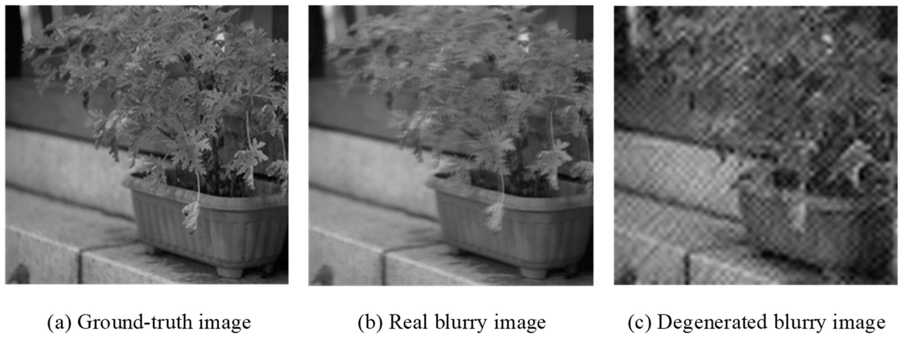
Validation of Degradation Model

In order to verify the reasonableness of our proposed degradation model, we performed degradation simulations on natural images. Illustrated in Figure 2, panels (a) and (b) depict a subset of scenes sourced from the Real-World Blur Dataset for learning and benchmarking deblurring algorithms [39]. Notably, panel (b) serves as the corresponding blur counterpart to the scene presented in panel (a) within the dataset. Employing our proposed degradation model, we subjected the GT image in panel (a) to degradation, resulting in the generation of the blurred image showcased in Figure 2c. Given the monochromatic nature of PET images, our initial preprocessing step involved the conversion of the three-channel natural image into a singular channel. Subsequently, we resized the image to achieve a square format, facilitating a more intuitive and visually discernible assessment of image degradation. This preparatory procedure was undertaken to enhance the clarity of observing the impact of degradation on the image. As depicted in Figure 2, our devised degradation methodology successfully simulated motion blur to a considerable extent, yielding promising outcomes. Nevertheless, it is imperative to acknowledge that variations in the simulated motion degree, coupled with the introduction of a moderate amount of additional noise, may contribute to subtle visual distinctions when compared to the authentic blurred images furnished for reference.

2.2. Proposed Architecture

Our objective was the training of a model, denoted as M, to acquire proficiency in learning non-linear mappings. This entailed the minimization of the mean squared error loss function, l_MSE, as delineated in Equation (20). Herein, we denoted the input LR image as y, output HR image as Y.

$$l_{MSE}=\frac{1}{n}{\displaystyle \sum _{i=1}^n{‖M(y_i)-Y_i‖}^2}$$

(20)

We addressed the following equation in the context of training images Y_i, where I = 1, ..., n, with n being the total number of training samples:

$$\widehat{Y}=\arg \min {\displaystyle \sum _{i=1}^n{l}_{MSE}(M(y_i),Y_i)}$$

(21)

$\widehat{Y}$ is the estimate of the target HR image, which is the generated SR image.

This subsection describes the principal constituents of our architecture y as depicted in Figure 3. Preserving the overarching design principles from the generator of SRGAN [30], we opted to excise the batch normalization (BN) layer. This strategic omission aimed to streamline the model’s complexity, fostering an enhancement in generalization capability. Although removing the BN layer may lead to slow convergence, unstable training, and easy overfitting, the residual connection maintained the identity mapping through the network layer, making it easier to optimize deeper networks and helping the model converge faster. Concurrently, the residual structure network in the deep residual can effectively solve the gradient flow and stability problems caused by removing the BN layer. Furthermore, the residual block architecture also aided in preventing overfitting. There are various ways to simplify the complexity of the model, but removing the BN layer is very consistent with using the residual network in the deep residual, which is the most direct way to balance the model among simplicity, training stability, and efficiency. Furthermore, we incorporated two successive parameterized rectified linear unit (PReLU) activation functions before the final output layer. This innovative integration is intended to empower the neural network to better handle non-linearity, enabling more effective learning and representation of intricate patterns in the data. The experimentation, expounded in Section 3.4, thoroughly substantiated the pivotal role played by the incorporation of two PReLUs. The tanh activation function was incorporated following the concluding convolution layer to expedite convergence throughout the training process. In tandem with this, we introduced an extensive skip connection, facilitating long-range information access. This architectural decision ensured the preservation of original data, mitigating any risk of data loss before the subsequent reconstruction process. Simultaneously, our approach introduced a feature extraction block—termed the deep residual-in-residual (DRRB), elucidated in Figure 3a. Motivated by the empirical observation that increased layers and interconnections invariably yield performance improvements, the proposed DRRB adopted a more complex and deeper structure within the SRGAN [30] generator, surpassing the ordinary residual block in terms of depth and complexity.

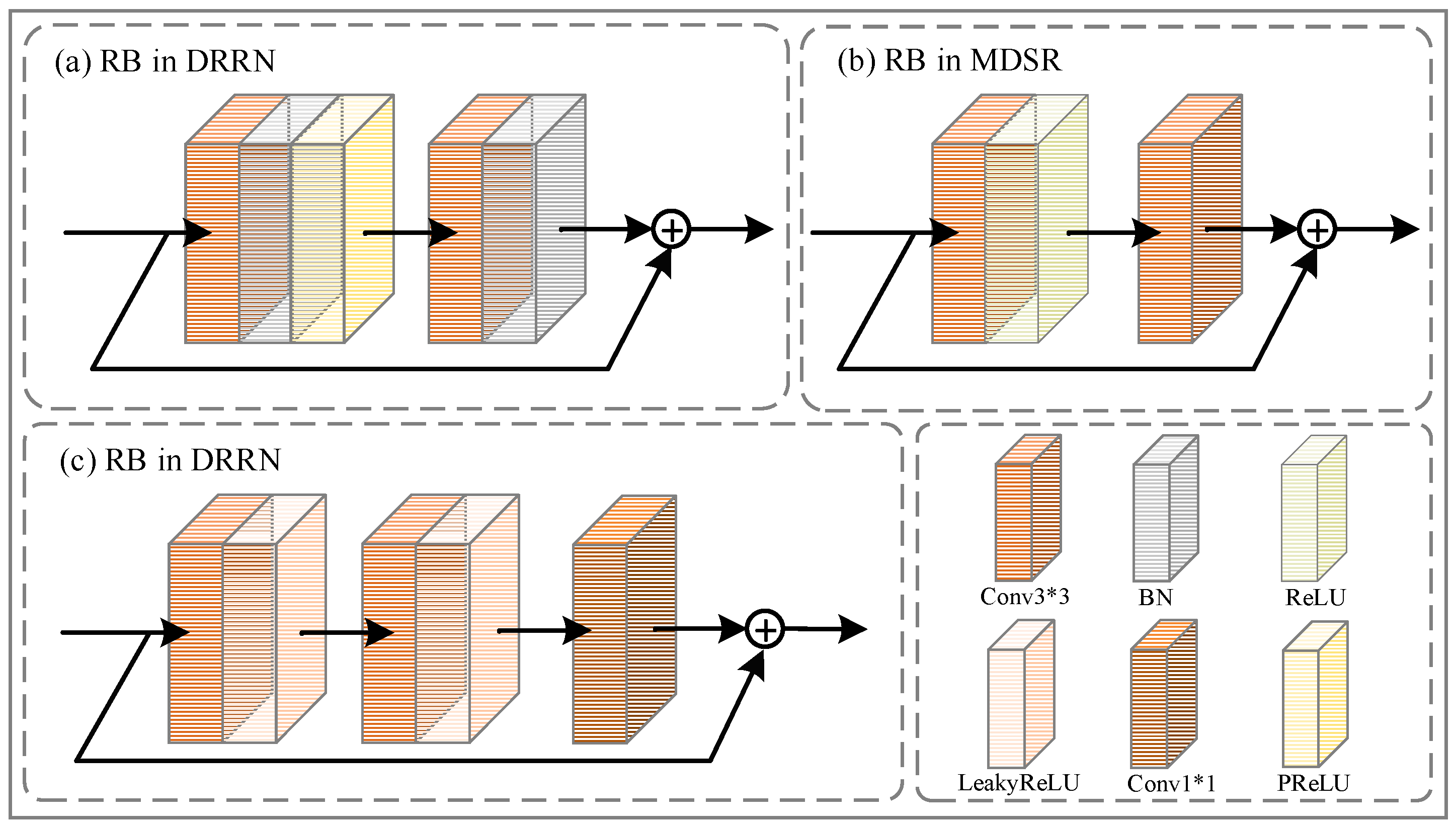
2.2.1. Deep Residual-in-Residual Block

To facilitate the acquisition of more intricate feature representations, we introduced a novel architectural refinement by embedding eleven basic residual blocks within the core structure of the residual block. This innovative approach aimed to significantly enhance the model’s ability to discern intricate details and textures critical for SR tasks. The entire deep residual-in-residual module, showcasing this nested design, is visually represented in Figure 3. The RIR structure not only provided an extended depth for the model but also profoundly augmented its nonlinear modeling capacity. The output of d-th RB in the RIR structure can be formulated as follows:

$$F_{RB}^d=f_{RB}^d(f_{RB}^{d-1}(\cdot \cdot \cdot f_{RB}^1(x)\cdot \cdot \cdot ))+x$$

(22)

This architectural augmentation, by virtue of the nested residual blocks, was strategically devised to empower the model with an enriched capacity to capture nuanced features and intricate patterns, ultimately contributing to its superior performance in this SR tasks.

2.2.2. Residual Block

Utilizing the conventional residual block (RB) [30] as a foundation, we proposed a novel RB structure aimed at improving the adaptability and efficiency of the RB. As can be observed in Figure 4, this architectural configuration used a dual-layer 3 × 3 convolutional architecture, departing from the structures used in SRGAN [30] and MDSR [40] by using a LeakyReLU activation (α = 0.2) rather than the PReLU activation and ReLU activation. The incorporation of LeakyReLU introduced a nuanced adaptability to the model when handling negative input regions, thereby enhancing the network’s overall expressive capacity. Notably, the outcomes of our investigations, detailed in Section 3.4, confirmed the superiority of LeakyReLU activation in the residual structure, surpassing the performance achieved with conventional ReLU activation. Drawing inspiration from the OverNet [41] architecture, we introduced a 1 × 1 convolution beneath the final layer of the RB module to dynamically merge output information and concurrently alleviate the computational complexity of the model. The formulation for the output of these hierarchical features is expressed as follows:

$$WA(x)=C_1(L(C_3(L(C_3(x)))))$$

(23)

$$f_{RB}={\lambda }_0(WA(x))+{\lambda }_{1}x$$

(24)

Here, we introduced the wide activation operation (WA) and denoted x and f_RB as the input and output vectors of the RB, respectively. Scalars λ₀ and λ₁ act as multipliers, contributing to the balance of data volume within the RBs of the network. Additionally, C₁ signifies 1 × 1 convolution, C₃ denotes 3 × 3 convolution, and L refers to LeakyReLU activation with the specified parameter.

2.3. Evaluation Metrics

In order to conduct a comprehensive and precise evaluation of the quality of SR PET images, we employed a set of five evaluation metrics. This encompassed a combination of full-reference metrics and no-reference metrics. Full-reference metrics gauge the similarity between the desired output and the authentic reference, while no-reference metrics focus on the internal features and structures of the image. The amalgamation of results from both types of metrics facilitates a more holistic understanding of all facets of PET image quality. This integrated approach serves as a more dependable guide for a thorough analysis of PET image quality and the optimization of tasks such as PET image generation and processing.

2.3.1. Full-Reference Evaluation

We conducted a rigorous evaluation of the image quality pertaining to SR PET images, employing three conventional and widely recognized metrics within the realms of image processing and computer vision: specifically, the peak signal-to-noise ratio (PSNR), the structural similarity index (SSIM), and the root mean square error (RMSE). In the subsequent delineations of metric definitions provided herein, we ascribed the appellations x and y to the actual and estimated images, respectively. The symbols μ and σ are employed to signify the mean and standard deviation in their respective capacities. Notably, MAX designates the peak grey level of the image, while MSE encapsulates the absolute mean square error. The quantification of the PSNR, MSE, SSIM, and RMSE are explicated through Equations (25)–(28).

$$PSNR=10\cdot {\log }_{10}\left(\frac{MA{X}^2}{MSE}\right)$$

(25)

$$MSE=\frac{1}{mn}{\displaystyle \sum _{i=0}^{m-1}{\displaystyle \sum _{j=0}^{n-1}\left(x_{ij}-y_{ij}\right)}}$$

(26)

$$SSIM=\frac{\left(2{\mu }_x{\mu }_y+c_1\right)\left(2{\sigma }_{xy}+c_2\right)}{({\mu }_x^2+{\mu }_y^2+c_1)({\sigma }_x^2+{\sigma }_y^2+c_2)}$$

(27)

Here, the parameters c₁ and c₂ serve the purpose of stabilizing the division operation.

$$RMSE=\sqrt{MSE}$$

(28)

2.3.2. No-Reference Evaluation

Given the absence of available ground truth images in establishing the fundamentals of the constructed SR method, we further evaluated the quality of SR images using two reference-free metrics. The first metric employed was the contrast-to-noise ratio (CNR), a widely utilized measure in PET image quality assessment. The CNR for a target region of interest (ROI) R and a reference ROI R_ref is defined in Equation (29).

$$CNR=\frac{\left|{\mu }^R-{\mu }^{R_{ref}}\right|}{\sqrt{\left[{\left({\sigma }^R\right)}^2+{\left({\sigma }^{R_{ref}}\right)}^2\right]}}$$

(29)

In this study, we selected the center of the image as the target ROI and selected the background areas of the image as the reference ROI.

The second metric was full width at half maximum (FWHM), offering insights into the width of peaks in the image and commonly utilized to evaluate the sharpness and resolving power of specific features. Smaller FWHM values show well-defined features in the image and better resolution. We fit the extracted pixel values using a Lorentzian function. The FWHM value of the fitted function curve was the measured FWHM result. The specific equations can be found in Equations (30) and (31).

$$FWHM=\gamma$$

(30)

$$l\left(\widehat{x}\right|A,x_{\ast },\mathsf{\gamma })=\frac{A}{1+{\left(\frac{\widehat{x}-x_{\ast }}{\mathsf{\gamma }}\right)}^2}$$

(31)

As shown in Equation (31), l represents the Lorentzian function. Among them, $\widehat{x}$ represents a one-dimensional array of pixel column data, γ denotes the FWHM resulting from the Lorentzian function fitting, and A represents the amplitude of the Lorentzian function, corresponding to the peak value. $x_{\ast }$ represents the abscissa of the peak value. The significance of FWHM lies in its ability to provide a numerical evaluation of how sharp an image’s edges are. Particularly in PET images and SR tasks, the precision of object edges is paramount for faithful image reproduction. By gauging FWHM, we can appraise the sharpness of object contours in an image, thereby gaining a deeper understanding of the tangible impact of SR methods on enhancing spatial resolution.

3. Experiments

3.1. Dataset

The small animal PET dataset (SAPET), acquired from the Metis^TM small animal PET/CT system, served as the training and validation dataset for assessing the performance of various SR models in enhancing PET image quality. The PET images were meticulously acquired and reconstructed by the researchers involved in this study, employing the ordered subsets expectation maximization (OSEM) method with 20 iterations and a matrix size of 257 × 257 × 389. The HR images utilized for training were obtained from the aforementioned PET scans, while the corresponding LR images were generated using the degradation model proposed in our study. The dataset comprised scans from ten mice, all anesthetized with chloral hydrate, injected with 500 μCi of 18-FDG, and left for 10 min prior to a 20-min scanning session. For the training phase, data from seven mice were employed, with one mouse for validation and two mice for testing. Additionally, a phantom dataset was used, acquired through scanning the Metis^TM, and reconstructed using OSEM with parameters matching the above mice scan. Prior to scanning, we injected phantoms with 18-FDG at a dose of 1000 μCi, and this phantom dataset served as an additional reference for assessing the robustness and generalization capabilities of the trained models.

Furthermore, the HR brain PET images from the Alzheimer’s Disease Neuroimaging Initiative (ADNI) [42] were included as exemplars for evaluation. A total of 34 cases were collected from the ADNI dataset (ADNID), all featuring a matrix size of 160 × 160 × 96. Fifteen cases were designated for training, with seven and twelve cases, respectively, allocated for validation and testing. The ADNI dataset provided a benchmark for assessing the performance of our proposed SR models in a clinical context.

3.2. Implementation Details

Performance experiments were conducted on the SAPET, phantom dataset, and ADNID to compare the proposed SR method with three classical SR networks, namely SRGAN [30], SRCNN [21], and VDSR [24]. The experiments were implemented using the PyTorch framework on an NVIDIA 3080 Ti graphics processing unit (GPU) for training.

The training parameters were configured as follows: Utilizing batches of size 8, momentum and weight decay parameters were set to 0.9 and 1 × 10⁻⁴, respectively. The training spanned 100 epochs, equivalent to 9725 iterations with a batch size of 8. The stochastic gradient descent method (SGD) was employed to train our proposed network, which was interconnected by multi-level jumpers, employing an adaptable learning rate strategy to derive a high-performing SR reconstruction model.

Specifically, the initial learning rates for the SAPET and phantom datasets were set at 0.3 and were subsequently decreased by 10% every 10 epochs. In the case of the ADNID model, the initial learning rate was established at 0.2, also decreasing by 10% every 10 epochs thereafter. These meticulous training configurations were designed to optimize the performance and convergence of the proposed SR method across diverse datasets. The parameter settings of the comparison models were consistent with those given in their papers.

In the context of degradation, the parameter ɛ in the Wiener filter was configured at 1 × 10⁻⁴. Throughout the experimental degradation process, the motion blur PSF was characterized by a fixed pixel value denoted as d, set at 5. This deliberate choice was made to emulate a smaller displacement distance, approximately 1.57 mm, simulating subtle movement. The motion angle, denoted as $\alpha$, was systematically varied across four experimental sets, specifically 0°, 10°, 20°, and 30°, meticulously chosen to replicate real-world scenarios of slight motion. This experimental framework was designed to delve into the nuanced impact of the SR model on image quality when confronted with varying degrees of subtle motion. The systematic manipulation of the motion angle allowed us to emulate the subtle movements of the imaged object in diverse orientations, facilitating an in-depth exploration of the repercussions of such motion on image quality.

3.3. Results

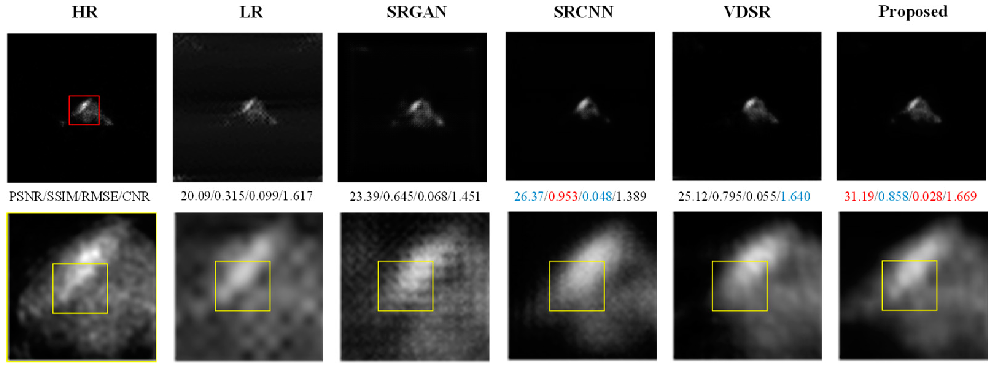
Comparison with Reference Methods

In the present study, our methodology entails the utilization of paired sets comprising degraded LR and HR images. We have conducted exhaustive training and thorough comparative analyses on faithfully replicated instances of SRGAN [30], SRCNN [21], VDSR [24], and our proposed DRRN. SRGAN [30] employs the GAN framework and introduces perceptual loss to generate SR images that are visually closer to real images with higher perceptual quality. Comparing it with SRGAN [30] helps to evaluate the visual quality improvement of our model. SRCNN [21], as the earliest deep learning SR model, serves as a benchmark for assessing new model advancements. VDSR [24], which incorporates residual learning and a deeper network structure, extracts rich features and produces higher quality SR images. Comparing it with VDSR [24] helps to evaluate the performance of our deep residual network in feature extraction and enhancement. These three models, ranging from basic to advanced, highlight our model’s improvements in visual quality, feature extraction, and computational efficiency. We commenced the study by degrading the input HR images. Subsequently, we employed an SR model to elevate the resolution of PET images, thereby showcasing the model’s effectiveness in ameliorating the resolution of motion-blurred images. Across the three datasets, we conducted experiments using four distinct degradation models to affirm the model’s reliability through qualitative and quantitative evaluations. The degradation scenarios, distinguished by motion angles, are systematically labeled: ‘case 1’ for a motion angle of 30°, ‘case 2’ for 20°, ‘case 3’ for 10°, and ‘case 4’ for 0°. The motion angles were incrementally augmented by 10° intervals, simulating subtle motions across varied angles. All of our LR images in the three datasets come from HR images using these four degradation methods. This meticulous approach ensures a comprehensive validation of the model’s dependability under diverse conditions, offering a nuanced assessment of its performance across a spectrum of motion angles.

On all three datasets, our method achieved convincing results. The absolute difference images in the SAPET dataset demonstrate that our method exhibits the smallest error in all cases, closest to the original HR image. However, as shown in

Table 1. SR quantitative results on the SAPET test set with different algorithms under four degradation approaches. The greatest and second-best performances are denoted by the colors red and blue, respectively.

Method	SAPET Case 1 PSNR/SSIM/RMSE/CNR	SAPET Case 2 PSNR/SSIM/RMSE/CNR	SAPET Case 3 PSNR/SSIM/RMSE/CNR	SAPET Case 4 PSNR/SSIM/RMSE/CNR
LR	24.57/0.776/0.061/2.164	23.30/0.745/0.071/2.035	23.31/0.755/0.071/2.120	18.55/0.733/0.120/1.921
SRGAN	24.60/0.733/0.063/1.939	23.99/0.751/0.067/1.866	23.56/0.693/0.071/1.864	22.46/0.677/0.080/1.747
SRCNN	28.70/0.899/0.039/1.939	28.61/0.886/0.040/1.897	27.85/0.887/0.043/1.917	25.37/0.872/0.058/1.951
VDSR	29.53/0.821/0.036/1.954	30.94/0.888/0.030/2.081	30.94/0.888/0.030/2.081	23.19/0.765/0.071/1.967
Proposed	34.36/0.913/0.020/2.085	33.03/0.898/0.024/2.024	31.61/0.899/0.028/2.035	30.18/0.879/0.033/2.039

, our proposed method is not as good as VDSR [24] in terms of CNR metrics in case 2 and 3, which are lower by 0.057 and 0.046, respectively. It can be seen that CNR metrics with high values do not guarantee visually good results, and it is still necessary to combine comprehensive metrics for evaluating the quality of the images. In the phantom dataset, although our proposed method is 0.57 dB lower than VDSR [24] in the PSNR and 0.005 dB higher than VDSR [24] in the RMSE in case 3, in Figure S9 (Supplementary Materials), it can be clearly seen that the highlights of VDSR [24] in the blue box are in different positions from those of the HR images; instead, our proposed method is closer to the reality. On the ADNI dataset, our method achieves the best results on all metrics. As shown in the absolute difference images, although in some cases our method does not recover the ROI as well as VDSR [24], it performs best in dealing with artefacts at the edges and four corners of the image.

A.

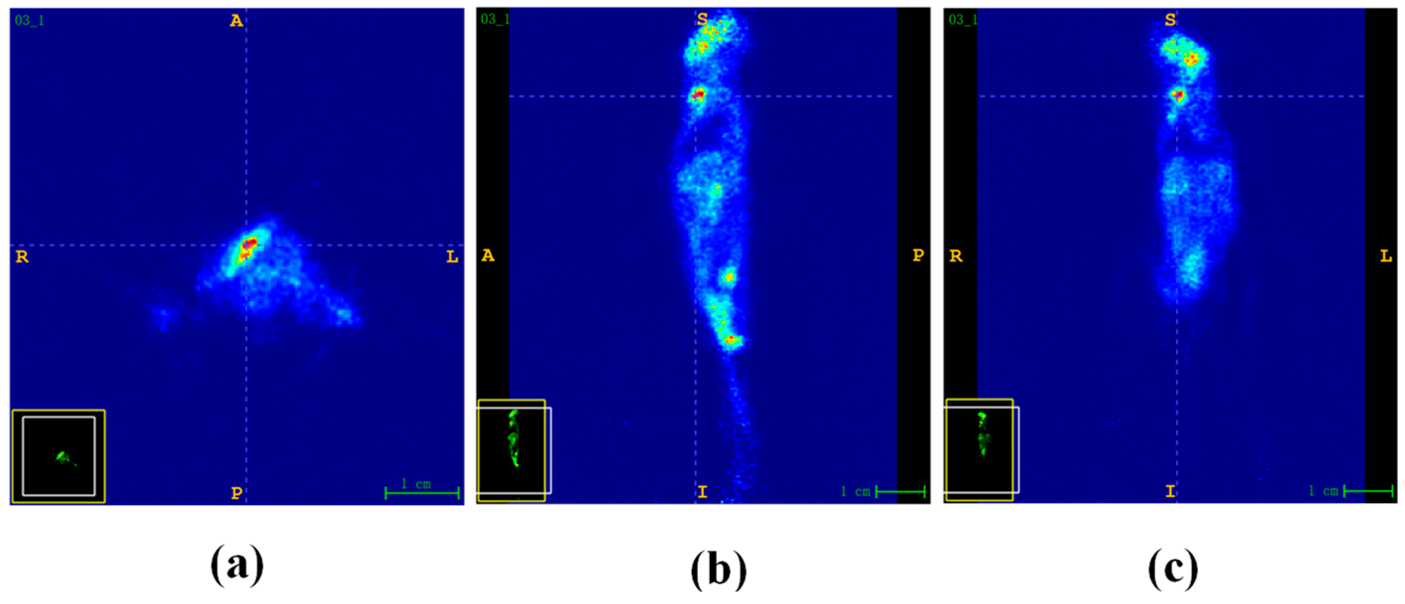
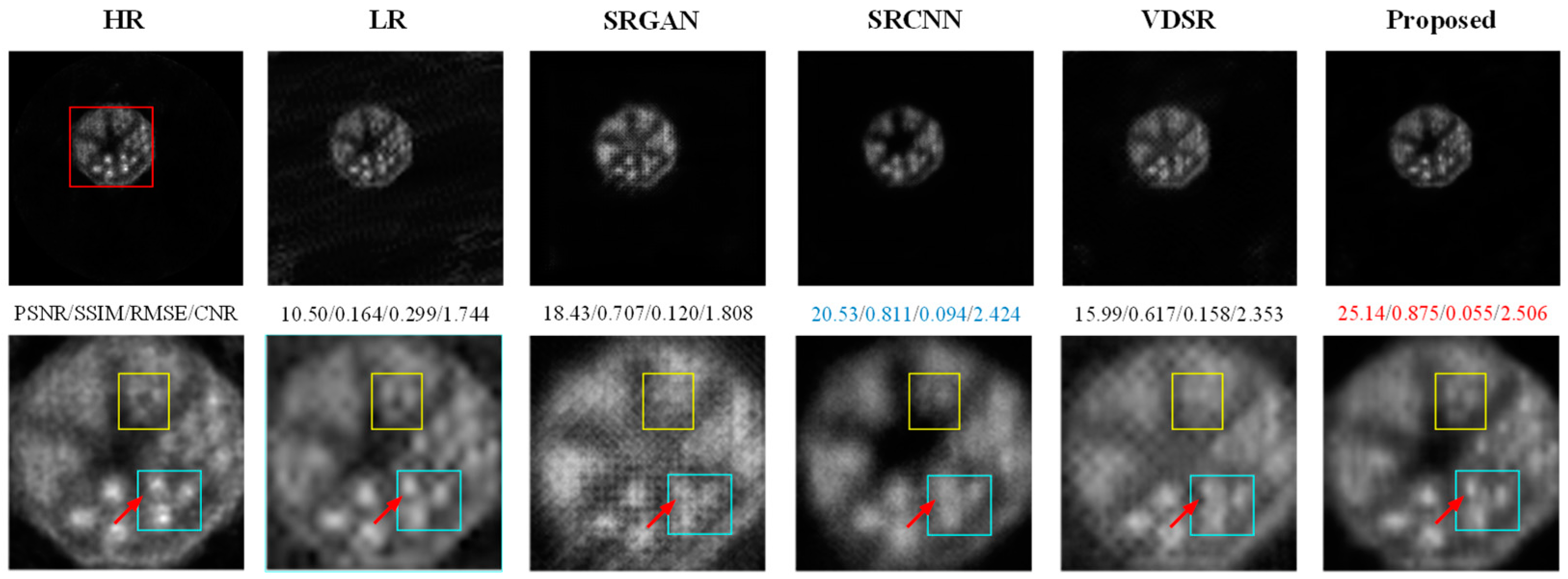
Results on the SAPET Dataset

Initially, our initial experimentation focused on preclinical imaging, specifically utilizing a dataset comprising mice, all of which exhibited lung cancer. The lesion is a tumor in the right posterior upper portion of the lung, close to the tip, as seen in Figure 5. We used sample PET slices with primary foci, as illustrated in Figure 6, chosen to visually assess the SR capabilities of various methodologies.

Overall, all methodologies exhibited a degree of efficacy in resolution enhancement. Illustrated in Figure 6, Figures S1, S2, and S6 (Supplementary Materials), both SRGAN [30] and SRCNN [21], yielded textures that deviated from the authentic HR images across the four distinct SR degradation methods. Particularly noteworthy is the region delineated by the yellow box, where SRGAN [30] and SRCNN [21] induced a discernible level of blurring in high-contrast lesions. On the other hand, although VDSR [24] performed better in detail processing than SRGAN [30] and SRCNN [21], it had disadvantages such as blurring in lesions with low contrast and the development of artefacts that resulted in a loss of texture information. Figure 7 and Figures S4–S6 (Supplementary Materials) display the difference images, which are generated by computing the difference between the HR image and the SR image pixel by pixel. The size and location of the difference are shown with color mapping. The difference image visually shows the difference between the generated SR image and the true HR image. By observing the difference image, we can quickly find out whether the SR model performs well in certain areas and show different degrees of ability to mitigate motion artifacts. Notably, our proposed method stands out with the most minimal error across all degradation methods, aligning closely with the original HR image.

All of the test set’s quantitative results are summarized in Table 1. The tabulated data clearly show that in terms of quantitative metrics, our proposed method performed better than the other methods in case 1 and case 4. To demonstrate the significant differences between the quantitative results of the proposed method and the results of the other three methods, statistical experiments were conducted. As shown in

Table 2. p-values of different methods on SAPET dataset.

Case 1/Case 2/Case 3/Case 4	PSNR↑	SSIM↑	RMSE↓	CNR↑
Proposed VS. SRGAN	<0.001/<0.001/ <0.001/<0.001	<0.001/<0.001/<0.001/<0.001	<0.001/<0.001/ <0.001/<0.001	<0.001/<0.001/ <0.001/<0.001
Proposed VS. SRCNN	<0.001/<0.001/ <0.001/<0.001	<0.001/<0.001/<0.001/<0.001	<0.001/<0.001/ <0.001/<0.001	<0.001/<0.001/ <0.001/<0.001
Proposed VS. VDSR	<0.001/<0.001/ <0.001/<0.001	<0.001/<0.001/<0.001/<0.001	<0.001/<0.001/ <0.001/<0.001	<0.001/=0.940/ =0.924/<0.001

, a p-value less than 0.01 indicates that all differences are statistically significant. In Table 1, on case 2 and case 3, although our proposed method is not as good as VDSR [24] in terms of the CNR, their p-values are all greater than 0.05 and are not statistically different. Consequently, our suggested method outperforms existing comparison methods in every way when the findings of the four indicators are combined.

B.

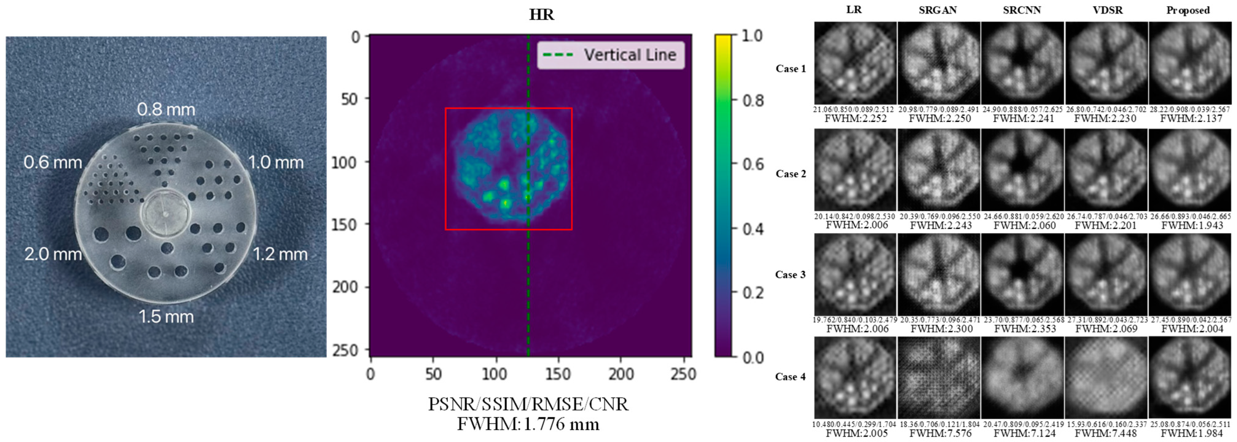
Results on the Phantom Dataset

In addition to the SAPET dataset, preclinical imaging datasets include phantom datasets. While motion blur is absent in phantoms, accurately measuring the FWHM in mouse PET images remains challenging, complicating the evaluation of the models’ effectiveness in improving spatial resolution. To address this, we have introduced mouse-like phantoms to assess various models’ capabilities in enhancing PET image spatial resolution and to comprehensively validate their robustness across different datasets.

We further compared the above-mentioned algorithms on the phantom dataset. A similar trend can be observed on this dataset. Our proposed method is substantially superior to other approaches that are closer to HR images for detail processing, especially on the detail image, as indicated by the region surrounded by the yellow box, and it can preserve high-frequency detail, as shown in Figure 8 and Figures S7–S9 (Supplementary Materials). It can also be observed by the ROIs pointed out by the red arrows that our proposed method removes the artefacts as well as suppresses the noise of the LR image to some extent. On the contrary, SRGAN [30], SRCNN [21], and VDSR [24] not only increase the artefacts but also show different degrees of textures that do not obey the HR image. In Figure 9 and Figures S10–S12 (Supplementary Materials), we showed the difference images by subtracting the generated image from the HR image. We compared our method with SRGAN [30], SRCNN [21], and VDSR [24] on the absolute difference images, and it is obvious that our method minimizes the error with respect to the HR image. However, the absolute difference images of the comparison methods have even larger errors than the absolute difference images of the LR image. This discrepancy serves as a compelling visual testament to the superior efficacy of our proposed method in minimizing errors and enhancing image fidelity.

Quantitative results for the phantom test set across various degradation cases are presented in

Table 3. SR quantitative results on the phantom test set with different algorithms under four degradation approaches. The greatest and second-best performances are denoted by the colors red and blue, respectively.

Method	Phantom Case 1 PSNR/SSIM/RMSE/CNR	Phantom Case 2 PSNR/SSIM/RMSE/CNR	Phantom Case 3 PSNR/SSIM/RMSE/CNR	Phantom Case 4 PSNR/SSIM/RMSE/CNR
LR	18.31/0.389/0.123/1.532	16.78/0.335/0.147/1.567	16.69/0.345/0.148/1.546	9.947/0.160/0.318/1.078
SRGAN	20.10/0.623/0.101/1.484	19.70/0.613/0.106/1.472	19.78/0.619/0.105/1.433	18.03/0.569/0.128/1.147
SRCNN	22.88/0.681/0.073/1.605	21.41/0.653/0.087/1.618	20.84/0.643/0.092/1.584	18.16/0.523/0.125/1.468
VDSR	24.93/0.702/0.058/1.620	23.51/0.666/0.068/1.658	24.00/0.657/0.064/1.610	11.44/0.432/0.273/1.421
Proposed	25.52/0.725/0.053/1.556	23.79/0.674/0.065/1.660	23.43/0.660/0.069/1.612	22.77/0.644/0.074/1.551

. Particularly in cases 4 and 2, our proposed method emerged as optimal across all metrics. In case 3, while our method did not surpass VDSR [24] in terms of the PSNR and RMSE metrics, the visual analysis, as depicted in Figure S9, elucidates nuances. Specifically, the highlights generated by our method in the region framed by the blue box on the detail image closely approximate the original HR image. Even though VDSR [24] performs well in certain metrics, it cannot reliably display the brightest points in the image, such as the highlights shown in Figures S7 and S9 by the red arrows. Moreover, the generated highlights’ shape deviates significantly from the HR diagram, clearly displaying artefacts beyond the blue box. To assess the statistical significance of quantitative differences between the proposed method and other comparative approaches, rigorous statistical experiments were conducted, and the corresponding p-values are delineated in

Table 4. p-values of different methods on phantom dataset.

Case 1/Case 2/Case 3/Case 4	PSNR↑	SSIM↑	RMSE↓	CNR↑
Proposed VS. SRGAN	<0.001/<0.001/ <0.001/<0.001	<0.001/<0.001/<0.001/<0.001	<0.001/<0.001/ <0.001/<0.001	<0.001/<0.001/ <0.001/<0.001
Proposed VS. SRCNN	<0.001/<0.001/ <0.001/<0.001	<0.001/<0.001/<0.001/<0.001	<0.001/<0.001/ <0.001/<0.001	=0.072<0.001/ <0.001/<0.001
Proposed VS. VDSR	<0.001/<0.001/ <0.001/<0.001	<0.001/<0.001/<0.001/<0.001	<0.001/<0.001/ <0.001/<0.001	=0.020/<0.001/ <0.001/<0.001

. Remarkably, in both case 2 and case 4, the p-values are less than 0.01, attesting that all observed differences attain a statistically significant level within these contexts. In case 1, a noteworthy observation is the p-value of the proposed method with SRCNN [21] on the CNR, recorded as 0.072. This specific value implies an absence of a statistically significant difference between the results of the two methods. Conversely, a discernible and statistically significant difference is evident between the proposed method and VDSR [24] on the CNR. An integrated analysis of Table 3 and Table 4 substantiates the superior performance of our proposed method across the majority of indicators in all cases compared to other comparative methods. Nevertheless, in case 1, our method falls short of matching VDSR [24] in the CNR, and in case 3, it does not surpass VDSR [24] in terms of the PSNR and RMSE. In order to evaluate the SR algorithm’s performance in greater depth, we also used FWHM independently to show the clarity of the image detail as shown in Figure 10, with smaller FWHM indicating better spatial resolution. To determine the best FWHM, we first identify an ROI in the brightest area of the phantom image and then extract the pixel values within the ROI along the direction of optimal focus as shown in the middle image of Figure 10. We then fit the extracted pixel values using a Lorentzian function as shown in Equation (31).

Table 5. The FWHM values on the phantom dataset with different algorithms under four degradation approaches. The greatest and second-best performances are denoted by the colors red and blue, respectively.

Method	Phantom Case 1 FWHM↓	Phantom Case 2 FWHM↓	Phantom Case 3 FWHM↓	Phantom Case 4 FWHM↓
LR	2.252	2.006	2.006	2.005
SRGAN	2.250	2.243	2.300	7.576
SRCNN	2.241	2.060	2.353	7.124
VDSR	2.230	2.201	2.069	7.448
Proposed	2.137	1.943	2.004	1.984

illustrates that our proposed SR method yields the lowest FWHM values across all cases. This outcome underscores its superior capability in enhancing spatial resolution compared to other comparative methods. In particular, noteworthy is the observation that in cases 2, 3, and 4, the FWHM values of SRGAN, SRCNN, and VDSR surpassed those of the LR images. This suggests a diminished efficacy in spatial detail restoration by these methods. In stark contrast, our SR method exhibited a remarkable ability to more effectively recover the high-frequency details of the images, thereby significantly improving the spatial resolution of the PET images. When all the quantitative findings are combined, our suggested method performs better than the reference methods in terms of metrics and visualization.

C.

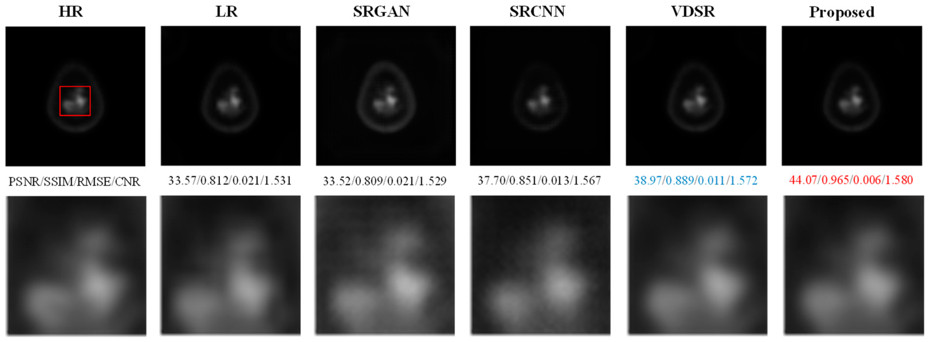
Results on the AD Dataset

In order to ascertain the reliability and implementability of the proposed methods, comprehensive experiments were conducted utilizing real clinical data from the ADNI dataset. The texture details in the HR images in this dataset that are inherently indistinct contribute to a scenario where visually discernible differences among the SR images generated by various methods are minimal, as illustrated in Figure 11, and what can be clearly seen is that SRGAN [30] and SRCNN [21] produce wrong textures. Figure 12 shows that our proposed method outperforms the other methods on all cases for small corners of the image edges, but on case 4, the absolute difference of our proposed method is greater than the other methods for the ROI circled by the red box. As shown in Figures S16–S18 (Supplementary Materials), on the detail images of the absolute difference images on cases 1, 2, and 3, the absolute difference of our proposed method is somewhat smaller than the other methods, but the difference is not very obvious compared to VDSR [24].

Table 6. SR quantitative results on the ADNI test set with different algorithms under four degradation approaches. The greatest and second-best performances are denoted by the colors red and blue, respectively.

Method	ADNI Case 1 PSNR/SSIM/RMSE/CNR	ADNI Case 2 PSNR/SSIM/RMSE/CNR	ADNI Case 3 PSNR/SSIM/RMSE/CNR	ADNI Case 4 PSNR/SSIM/RMSE/CNR
LR	32.39/0.819/0.024/1.457	32.55/0.824/0.023/1.460	32.97/0.832/0.022/1.469	33.71/0.842/0.021/1.491
SRGAN	34.33/0.861/0.019/1.481	33.74/0.822/0.021/1.457	33.78/0.820/0.020/1.460	33.72/0.818/0.021/1.457
SRCNN	37.62/0.853/0.013/1.500	37.58/0.850/0.013/1.497	37.56/0.850/0.013/1.497	37.49/0.848/0.013/1.495
VDSR	42.45/0.938/0.008/1.507	40.34/0.910/0.010/1.505	39.14/0.892/0.011/1.503	38.62/0.882/0.012/1.503
Proposed	44.13/0.966/0.006/1.513	43.13/0.957/0.007/1.513	43.26/0.959/0.007/1.512	42.81/0.968/0.007/1.507

shows the quantitative results of the various methods on ADNI data under different degradation cases, and the results show that our proposed method is higher than the other comparative methods in all evaluation indexes regardless of the cases. To establish the statistical significance of the observed differences in quantitative results between the proposed method and the three other comparative methods, rigorous statistical experiments were conducted, and the corresponding p-values are presented in

Table 7. p-values of different methods on ADNI dataset.

Case 1/Case 2/Case 3/Case 4	PSNR↑	SSIM↑	RMSE↓	CNR↑
Proposed VS. SRGAN	<0.001/<0.001/ <0.001/<0.001	<0.001/<0.001/<0.001/<0.001	<0.001/<0.001/ <0.001/<0.001	<0.001/<0.001/<0.001/<0.001
Proposed VS. SRCNN	<0.001/<0.001/ <0.001/<0.001	<0.001/<0.001/<0.001/<0.001	<0.001/<0.001/ <0.001/<0.001	<0.001/<0.001/<0.001/<0.001
Proposed VS. VDSR	<0.001/<0.001/<0.001/<0.001	<0.001/<0.001/<0.001/<0.001	<0.001/<0.001/ <0.001/<0.001	<0.001/<0.001/<0.001/<0.001

. All computed p-values are found to be less than 0.01, underscoring the statistical significance of the disparities observed in the evaluation metrics. This outcome serves as a robust validation, indicating that the differences in performance metrics between the proposed method and the comparative networks are not merely coincidental but indeed demonstrate a significant and systematic distinction.

3.4. Ablation and Super Parameter Experiments

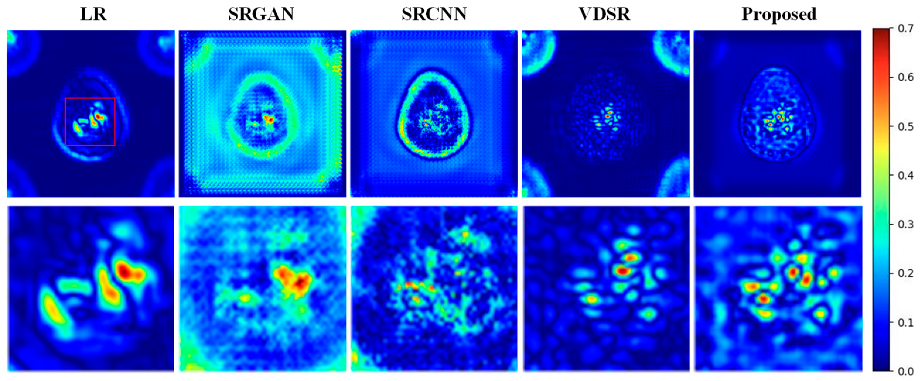
In this subsection, we conducted ablation and super parameter experiments to assess the efficacy of the model-related enhancements proposed in Section 3.2. Al experiments were performed on case 4 of the SAPET dataset. Diverging from the conventional-based Residual Block (RB) module that employs ReLU activation, we opted for LeakyReLU throughout all modifications. The experimental results shown in

Table 8. p-values of different methods on ADNI dataset.

Design	PSNR↑	SSIM↑	RMSE↓
RB with ReLU	29.49	0.878	0.036
RB with PReLU	27.02	0.950	0.048
RB with LeakyReLU	30.18	0.879	0.033

unequivocally show that LeakyReLU introduces more nonlinear transformations than ReLU and PReLU, which improves the PSNR significantly and helps the network fit complex function mappings better. It also makes high-frequency detail recovery for the SR task easier. In addition, LeakyReLU’s non-zero gradient makes it easier for gradients to be back propagated in deep networks, preventing the disappearing gradient issue and improving the network’s ability to learn deep features. Intriguingly, the empirical evidence suggests that the use of ReLU activation in deeper networks does not produce superior performance across all metrics, highlighting the limitations of this conventional activation function in mitigating issues associated with vanishing gradients.

Before the final output layer of the model, we use two consecutive PReLU activations to make the model training more stable. The PReLU activations can adapt more flexibly to the differences in the image details and texture distributions, which improves the expressive power of the network. Also, the model can adaptively learn the activation pattern in the negative input region according to the characteristics of the data to better fit the data distribution. As shown in

Table 9. Super parameter experiments on the number of PReLU activation functions before the final output layer.

Design	PSNR↑	SSIM↑	RMSE↓
0	27.19	0.872	0.047
1	29.07	0.880	0.038
2	30.18	0.879	0.033
3	28.80	0.879	0.039

, the numbers in the first column represent the number of consecutive PLeLU activation functions before the final output layer. The optimal value of the PSNR occurs when there are two PReLU activation functions.

4. Discussion

PET images are significantly constrained in spatial resolution due to various physical and technical imaging factors, often to a greater extent than anatomical imaging modalities, such as MR and CT. This limitation directly impacts the precise localization and in-depth analysis of small lesions and biological processes. SR, as an image processing technique, is dedicated to improving the quality of functional imaging, such as PET, by improving the spatial resolution of images. Therefore, SR has a special importance in enhancing the quality of PET images.

Our task in this study is to improve the resolution of PET images with deep learning without upgrading hardware devices. In the context of natural image SR tasks, numerous methods employ bicubic downsampling kernels to yield visually appealing outcomes. Since the SR problem is an inverse problem and the fidelity of LR images is crucial for reconstructing SR images, the use of a bicubic downsampling kernel is often impractical to apply to medical images. Presently, SR techniques for medical images primarily rely on generic degradation models, lacking tailored approaches for real-world scanning scenarios. During PET image acquisition, patients may undergo involuntary physiological movements, and even subtle tremors can detrimentally impact image quality. Considering the artefacts stemming from these physiological movements, it becomes imperative to simulate linear motion induced by patient physiological movements during scanning to enhance PET image quality. Therefore, a new degradation method is proposed by us, aiming to simulate linear motion artefacts induced by physiological motion during PET image scanning. In comparison with traditional generalized degradation methods, our approach achieves a closer emulation of the real scanning environment and more efficiently captures image degradation caused by physiological motion. In terms of existing research, although some studies have attempted SR methods for PET images, the majority have not addressed the challenges posed by physiological movements during PET image scanning. Therefore, this work fills a critical gap and provides a novel and more suitable solution for medical image SR tasks in practical applications.

As shown in the absolute difference images of Figure 7 and Figures S4–S6, SRCNN excels in capturing high-frequency edge details due to its smaller receptive field, resulting in better edge artifact suppression compared to VDSR. However, its shallow network structure hinders its ability to effectively model complex low-frequency texture structures in the ROI. Conversely, VDSR’s larger receptive field enables a superior reconstruction of low-frequency textures in the ROI, but it struggles with preserving high-frequency edge information due to potential information loss during deep propagation. As shown in Figure 10 and Table 5, as the motion blur angle approaches 0°, the traditional SR models, SRGAN, SRCNN, and VDSR, perform poorly in the SR task. The FWHM value of the generated image exceeds that of the LR image, especially when the motion blur kernel appears horizontally linear. This phenomenon can be attributed to the SRGAN generator network’s use of large receptive field convolutional layers, which focus on capturing the global structural features of the image, making it difficult to accurately reconstruct fine details. The shallow network structure of SRCNN fails to adequately capture and reconstruct image details. While VDSR increases the network depth to enhance the global feature extraction capability, it still lacks the sufficient modeling of local detailed information. When the motion blur kernel presents a horizontal linear form, it leads to the loss of more horizontal edges and details, posing a significant challenge for the aforementioned models. We suggest the DRRN structure in light of the drawbacks of conventional SR methods, which enables input data to be directly transferred to later levels, maintaining the specifics and edge data from the initial input in the process. The residual-in-residual design allows for each layer to reuse the feature information from earlier layers while also learning new feature representations. This makes it easier for the model to use and integrate multi-level information, which improves its capacity to learn and reconstruct edge and detailed features. As a result, our method greatly improves spatial resolution, outperforming conventional models in every case. In conjunction with Figure 6 and Figures S1–S3, our proposed method achieves an efficient fusion of high- and low-frequency information. It can be seen that it outperforms SRGAN, SRCNN, and VDSR in both edge artifact suppression and ROI texture recovery, validating its superior performance in the PET image super-resolution task. Our method is mainly validated on the preclinical SAPET dataset, the phantom dataset, and the AD dataset as a validation of the robustness of the model. Image quality is assessed in a multifaceted way by introducing full-reference metrics and no-reference metrics.

In accordance with the absolute difference image depicted in Figure 13, our proposed method unequivocally demonstrates the minimal error and optimal performance in case 4. By comparing the LR image data in Table 1, it becomes apparent that case 4 experiences a reduction in the PSNR by 6.02 dB compared to case 1, 4.75 dB compared to case 2, and concomitantly, a parallel diminution of 4.76 dB compared to case 3. Moreover, when considering alternative metrics, case 4 manifests relatively poor values, indicative of an elevated degradation in the LR images associated with this particular scenario. It is imperative to underscore that notwithstanding the heightened quality degradation in the LR image generated by case 4, it paradoxically exhibits the most minimal error in the SR image when compared to the other cases. This paradox underscores the efficacy of our proposed method, suggesting an augmented restorative capacity when addressing low-quality LR images. This result laterally confirms the significant advantage of our method in processing PET images with motion blur. These findings not only emphasize the effectiveness of our proposed method in recovering low-quality PET images but also highlight its superior performance in coping with motion blur. This has a positive impact on improving PET image quality and enhancing the diagnosis and analysis of medical images.

This study focused on preclinical PET imaging, where inadequate anesthesia can lead to movement in mice, exacerbated by physiological twitching. In clinical PET imaging, patient discomfort can result in involuntary movements. To address these challenges, introducing motion blur and artifacts is necessary. Specific suitable parameter settings were used in the degradation process. The noise level $\epsilon$ is set to 1 × 10⁻⁴ to simulate weak noise, ensuring that the noise level in the LR image is subtle and does not overshadow the main research objectives. A displacement distance of d = 5 pixels, equivalent to 1.57 mm, effectively simulates artifacts from slight motion, striking a balance between subtle blur and detail retention. If d is too small, it fails to realistically simulate blur; if too large, it causes excessive blur, negatively impacting SR reconstruction. Despite the convincing results of our model, there are still some limitations. First, given the unsatisfactory ROI retrieval performance in our proposed method for clinical datasets, future research directions will focus on designing more efficient architectures. We plan to draw on the relatively simplified method proposed in this study by constructing a more effective network structure in order to learn more fully the complex structural features in the clinical data and to validate its effectiveness through comprehensive experiments. Second, the degradation approach proposed in this study to simulate the blurring caused by the motion of a small animal in a specific direction during scanning is more realistic compared to other medical image SR methods that use interpolation to degrade an image under ideal conditions. However, considering that the physiological movements of patients in real clinics may be more complex, subsequent studies will further deepen the simulation of clinical images in order to design degradation models that are more realistic and applicable to patient situations. Future research directions also include the design of PET SR methods with multimodal inputs to make a more comprehensive use of clinical data and provide personalized services to patients. Consider utilizing cross-modal transfer learning to transfer the model’s learned experiences from PET images to other imaging modalities, such as MRI and CT. This approach enables the model to adapt to various medical imaging modes, thereby enhancing its application potential across diverse medical imaging tasks.

5. Conclusions

In this study, we propose a deep learning-based PET image SR. In contrast to traditional medical image SR, our method is modeled in a more realistically damaged environment rather than an idealized one. We take into account scenarios that could arise during scanning, such as motion artefacts brought on by the moving item being scanned. We create a more realistic degradation model and propose a network called DRRN based on a deep residual-in-residual structure for SR reconstruction of low-quality PET images to SR images in a more realistic situation. We used three distinct datasets to evaluate the implemented DRRN. The findings demonstrate that when compared to other approaches, our suggested DRRN produces notable benefits in both qualitative and quantitative assessments. Furthermore, we assess the ability to improve spatial resolution by calculating the FWHM, and the findings demonstrate the DRRN’s notable advantage in this area. In summary, the proposed DRRN has demonstrated efficacy in PET image SR, has shown potential for clinical applications and may somewhat reduce the impacts of motion blur.

References

1. Ametamey, S.M.; Honer, M.; Schubiger, P.A. Molecular Imaging with PET. Chem. Rev. 2008, 108, 1501–1516. [Google Scholar] [CrossRef] [PubMed]
2. Wollring, M.M.; Werner, J.-M.; Ceccon, G.; Lohmann, P.; Filss, C.P.; Fink, G.R.; Langen, K.-J.; Galldiks, N. Clinical Applications and Prospects of PET Imaging in Patients with IDH-Mutant Gliomas. J. Neurooncol. 2023, 162, 481–488. [Google Scholar] [CrossRef] [PubMed]
3. Subramanyam Rallabandi, V.P.; Seetharaman, K. Deep Learning-Based Classification of Healthy Aging Controls, Mild Cognitive Impairment and Alzheimer’s Disease Using Fusion of MRI-PET Imaging. Biomed. Signal Process. Control 2023, 80, 104312. [Google Scholar] [CrossRef]
4. Romeo, V.; Moy, L.; Pinker, K. AI-Enhanced PET and MR Imaging for Patients with Breast Cancer. PET Clin. 2023, 18, 567–575. [Google Scholar] [CrossRef] [PubMed]
5. Aitken, M.; Chan, M.V.; Urzua Fresno, C.; Farrell, A.; Islam, N.; McInnes, M.D.F.; Iwanochko, M.; Balter, M.; Moayedi, Y.; Thavendiranathan, P.; et al. Diagnostic Accuracy of Cardiac MRI versus FDG PET for Cardiac Sarcoidosis: A Systematic Review and Meta-Analysis. Radiology 2022, 304, 566–579. [Google Scholar] [CrossRef] [PubMed]
6. Cherry, S.R. Of Mice and Men (and Positrons)—Advances in PET Imaging Technology. J. Nucl. Med. 2006, 47, 1735–1745. [Google Scholar] [PubMed]
7. Feng, L. 4D Golden-Angle Radial MRI at Subsecond Temporal Resolution. NMR Biomed. 2023, 36, e4844. [Google Scholar] [CrossRef] [PubMed]
8. Shah, A.; Rojas, C.A. Imaging Modalities (MRI, CT, PET/CT), Indications, Differential Diagnosis and Imaging Characteristics of Cystic Mediastinal Masses: A Review. Mediastinum 2023, 7, 3. [Google Scholar] [CrossRef] [PubMed]
9. Wang, G.; Yu, H.; De Man, B. An Outlook on X-ray CT Research and Development. Med. Phys. 2008, 35, 1051–1064. [Google Scholar] [CrossRef]
10. Braams, J.W.; Pruim, J.; Freling, N.J.M.; Nikkeis, P.G.J.; Roodenburg, J.L.N.; Boering, G.; Vaalburg, W.; Vermey, A.; Braams, J.W. Detection of Lymph Node Metastases of Squamous-Cell Cancer of the Head and Neck with FDG-PET and MRI. J. Nucl. Med. 1995, 36, 211–216. [Google Scholar]
11. Kitajima, K.; Murakami, K.; Yamasaki, E.; Kaji, Y.; Sugimura, K. Accuracy of Integrated FDG-PET/Contrast-Enhanced CT in Detecting Pelvic and Paraaortic Lymph Node Metastasis in Patients with Uterine Cancer. Eur. Radiol. 2009, 19, 1529–1536. [Google Scholar] [CrossRef] [PubMed]
12. Chen, S.; Tian, X.; Wang, Y.; Song, Y.; Zhang, Y.; Zhao, J.; Chen, J.-C. DAEGAN: Generative Adversarial Network Based on Dual-Domain Attention-Enhanced Encoder-Decoder for Low-Dose PET Imaging. Biomed. Signal Process. Control 2023, 86, 105197. [Google Scholar] [CrossRef]
13. Cao, K.; Xia, Y.; Yao, J.; Han, X.; Lambert, L.; Zhang, T.; Tang, W.; Jin, G.; Jiang, H.; Fang, X.; et al. Large-Scale Pancreatic Cancer Detection via Non-Contrast CT and Deep Learning. Nat. Med. 2023, 29, 3033–3043. [Google Scholar] [CrossRef] [PubMed]
14. Umirzakova, S.; Ahmad, S.; Khan, L.U.; Whangbo, T. Medical Image Super-Resolution for Smart Healthcare Applications: A Comprehensive Survey. Inf. Fusion 2024, 103, 102075. [Google Scholar] [CrossRef]
15. Zhou, F.; Yang, W.; Liao, Q. Interpolation-Based Image Super-Resolution Using Multisurface Fitting. IEEE Trans. Image Process. 2012, 21, 3312–3318. [Google Scholar] [CrossRef] [PubMed]
16. Ahmad, T.; Li, X.M. An Integrated Interpolation-Based Super Resolution Reconstruction Algorithm for Video Surveillance. J. Commun. 2012, 7, 464–472. [Google Scholar] [CrossRef]
17. Tanaka, M.; Okutomi, M. Theoretical Analysis on Reconstruction-Based Super-Resolution for an Arbitrary PSF. In Proceedings of the 2005 IEEE Computer Society Conference on Computer Vision and Pattern Recognition (CVPR’05), San Diego, CA, USA, 20–25 June 2005; IEEE: New York, NY, USA; pp. 947–954. [Google Scholar]
18. Fan, C.; Wu, C.; Li, G.; Ma, J. Projections onto Convex Sets Super-Resolution Reconstruction Based on Point Spread Function Estimation of Low-Resolution Remote Sensing Images. Sensors 2017, 17, 362. [Google Scholar] [CrossRef] [PubMed]
19. Huang, X.; Jiang, Y.; Liu, X.; Xu, H.; Han, Z.; Rong, H.; Yang, H.; Yan, M.; Yu, H. Machine Learning Based Single-Frame Super-Resolution Processing for Lensless Blood Cell Counting. Sensors 2016, 16, 1836. [Google Scholar] [CrossRef] [PubMed]
20. Jia, K.; Wang, X.; Tang, X. Image Transformation Based on Learning Dictionaries across Image Spaces. IEEE Trans. Pattern Anal. Mach. Intell. 2013, 35, 367–380. [Google Scholar] [CrossRef]
21. Dong, C.; Loy, C.C.; He, K.; Tang, X. Image Super-Resolution Using Deep Convolutional Networks. IEEE Trans. Pattern Anal. Mach. Intell. 2016, 38, 295–307. [Google Scholar] [CrossRef]
22. Dong, C.; Loy, C.C.; Tang, X. Accelerating the Super-Resolution Convolutional Neural Network. In Proceedings of the Computer Vision–ECCV 2016: 14th European Conference, Amsterdam, The Netherlands, 11–14 October 2016; Proceedings, Part II 14. pp. 391–407. [Google Scholar] [CrossRef]
23. Shi, W.; Caballero, J.; Huszár, F.; Totz, J.; Aitken, A.P.; Bishop, R.; Rueckert, D.; Wang, Z. Real-Time Single Image and Video Super-Resolution Using an Efficient Sub-Pixel Convolutional Neural Network. In Proceedings of the IEEE Conference on Computer Vision and Pattern Recognition (CVPR), Las Vegas, NV, USA, 26 June–1 July 2016. [Google Scholar]
24. Kim, J.; Lee, J.K.; Lee, K.M. Accurate Image Super-Resolution Using Very Deep Convolutional Networks. In Proceedings of the 2016 IEEE Conference on Computer Vision and Pattern Recognition (CVPR), Las Vegas, NV, USA, 26 June–1 July 2016; pp. 1646–1654. [Google Scholar]
25. Zhang, Y.; Li, K.; Li, K.; Wang, L.; Zhong, B.; Fu, Y. Image Super-Resolution Using Very Deep Residual Channel Attention Networks. In Proceedings of the European Conference on Computer Vision (ECCV), Munich, Germany, 8–14 September 2018; pp. 294–310. [Google Scholar]
26. Qiu, D.; Zhang, S.; Liu, Y.; Zhu, J.; Zheng, L. Super-Resolution Reconstruction of Knee Magnetic Resonance Imaging Based on Deep Learning. Comput. Methods Programs Biomed. 2020, 187, 105059. [Google Scholar] [CrossRef]
27. Song, T.-A.; Chowdhury, S.R.; Yang, F.; Dutta, J. Super-Resolution PET Imaging Using Convolutional Neural Networks. IEEE Trans. Comput. Imaging 2020, 6, 518–528. [Google Scholar] [CrossRef]
28. Qiu, D.; Cheng, Y.; Wang, X. Improved Generative Adversarial Network for Retinal Image Super-Resolution. Comput. Methods Programs Biomed. 2022, 225, 106995. [Google Scholar] [CrossRef]
29. Zhu, D.; He, H.; Wang, D. Feedback Attention Network for Cardiac Magnetic Resonance Imaging Super-Resolution. Comput. Methods Programs Biomed. 2023, 231, 107313. [Google Scholar] [CrossRef]
30. Ledig, C.; Theis, L.; Huszar, F.; Caballero, J.; Cunningham, A.; Acosta, A.; Aitken, A.; Tejani, A.; Totz, J.; Wang, Z.; et al. Photo-Realistic Single Image Super-Resolution Using a Generative Adversarial Network. In Proceedings of the 2017 IEEE Conference on Computer Vision and Pattern Recognition (CVPR), Honolulu, HI, USA, 21–26 July 2017; pp. 105–114. [Google Scholar]
31. Tian, X.; Chen, S.; Wang, Y.; Zhao, J.; Chen, J. PET Imaging Super-Resolution Using Attention-Enhanced Global Residual Dense Network. In Proceedings of the 2023 IEEE 3rd International Conference on Computer Systems (ICCS), Qingdao, China, 22–24 September 2023; pp. 91–98. [Google Scholar]
32. Qiu, D.; Zheng, L.; Zhu, J.; Huang, D. Multiple Improved Residual Networks for Medical Image Super-Resolution. Future Gener. Comput. Syst. 2021, 116, 200–208. [Google Scholar] [CrossRef]
33. Zhu, D.; Sun, D.; Wang, D. Dual Attention Mechanism Network for Lung Cancer Images Super-Resolution. Comput. Methods Programs Biomed. 2022, 226, 107101. [Google Scholar] [CrossRef]
34. Song, T.-A.; Chowdhury, S.R.; Yang, F.; Dutta, J. PET Image Super-Resolution Using Generative Adversarial Networks. Neural Netw. 2020, 125, 83–91. [Google Scholar] [CrossRef]
35. Park, S.-J.; Ionascu, D.; Killoran, J.; Mamede, M.; Gerbaudo, V.H.; Chin, L.; Berbeco, R. Evaluation of the Combined Effects of Target Size, Respiratory Motion and Background Activity on 3D and 4D PET/CT Images. Phys. Med. Biol. 2008, 53, 3661–3679. [Google Scholar] [CrossRef] [PubMed]
36. Elad, M.; Hel-Or, Y. A fast super-resolution reconstruction algorithm for pure translational motion and common space-invariant blur. In Proceedings of the 21st IEEE Convention of the Electrical and Electronic Engineers in Israel, Tel-Aviv, Israel, 11–12 April 2000; Proceedings (Cat. No.00EX377). pp. 402–405. [Google Scholar] [CrossRef]
37. Elad, M.; Feuer, A. Restoration of a Single Superresolution Image from Several Blurred, Noisy, and Undersampled Measured Images. IEEE Trans. Image Process. 1997, 6, 1646–1658. [Google Scholar] [CrossRef] [PubMed]
38. Wang, X.; Xie, L.; Dong, C.; Shan, Y. Real-ESRGAN: Training Real-World Blind Super-Resolution with Pure Synthetic Data. In Proceedings of the 2021 IEEE/CVF International Conference on Computer Vision Workshops (ICCVW), Montreal, BC, Canada, 17 October 2021; pp. 1905–1914. [Google Scholar]
39. Rim, J.; Lee, H.; Won, J.; Cho, S. Real-World Blur Dataset for Learning and Benchmarking Deblurring Algorithms. In Proceedings of the Computer Vision–ECCV 2020: 16th European Conference, Glasgow, UK, 23–28 August 2020; Proceedings, Part XXV 16. pp. 184–201. [Google Scholar] [CrossRef]
40. Lim, B.; Son, S.; Kim, H.; Nah, S.; Lee, K.M. Enhanced Deep Residual Networks for Single Image Super-Resolution. In Proceedings of the IEEE Conference on Computer Vision and Pattern Recognition Workshops, Honolulu, HI, USA, 21–26 July 2017; pp. 136–144. [Google Scholar]
41. Behjati, P.; Rodriguez, P.; Mehri, A.; Hupont, I.; Tena, C.F.; Gonzalez, J. OverNet: Lightweight Multi-Scale Super-Resolution with Overscaling Network. In Proceedings of the 2021 IEEE Winter Conference on Applications of Computer Vision (WACV), Waikoloa, HI, USA, 3–8 January 2021; pp. 2693–2702. [Google Scholar]
42. Alzheimer’s Disease Neuroimaging Initiative (ADNI). Available online: https://adni.loni.usc.edu/data-samples/access-data/ (accessed on 11 January 2023).
43. itk-SNAP. Available online: http://www.itksnap.org/pmwiki/pmwiki.php (accessed on 11 January 2023).
Figure 1. General architectural diagram of our SR mission.
Electronics 13 02582 g001
Figure 2. The comparative images of the GT image, real blurry image, and degraded image of the natural image.
Electronics 13 02582 g002
Figure 3. The architecture of our proposed deep residual-in-residual network (DRRN).
Electronics 13 02582 g003
Figure 4. Comparison of prior network structures (a,b) and our residual dense block (c). (a) RB in SRGAN [30]. (b) RB in MDSR [40]. (c) Our RB.
Electronics 13 02582 g004
Figure 5. A cross-sectional image of a mouse for the matching HR image in Figure 6 is shown in figure (a). This mouse’s coronal image is shown in (b), and its sagittal image is shown in (c). The red highlighted area localized in the image is the primary lung cancer lesion. All images in this figure were generated by the software ITK-SNAP 3.8.0 [43].
Electronics 13 02582 g005
Figure 6. Case 4 in the SAPET dataset is visually compared. The second row of images is the ROI zoomed in on the first row of images marked with a red rectangle. The red font below the image indicates the best result, and the blue font indicates the suboptimal result.
Electronics 13 02582 g006
Figure 7. Absolute difference images relative to the original HR image from case 4 of the SAPET dataset. The second row of images is the ROI zoomed in on the first row of images marked with a red rectangle.
Electronics 13 02582 g007
Figure 8. Case 4 in the phantom dataset is visually compared. The second row of images is the ROI zoomed in on the first row of images marked with a red rectangle.
Electronics 13 02582 g008
Figure 9. Absolute difference images relative to the original HR image from case 4 of the phantom dataset. The second row of images is the ROI zoomed in on the first row of images marked with a red rectangle.
Electronics 13 02582 g009
Figure 10. The left picture is a photograph of the phantom. The middle image is the HR image, where the green dashed line is the dashed line drawn at the brightest ROI selected. The right image shows the FWHM values measured by different methods in 4 cases and the resulting images.
Electronics 13 02582 g010
Figure 11. Case 4 in the ADNI dataset is visually compared. The second row of images is the ROI zoomed in on the first row of images marked with a red rectangle.
Electronics 13 02582 g011
Figure 12. Absolute difference images relative to the original HR image from case 4 of the ADNI dataset. The second row of images is the ROI zoomed in on the first row of images marked with a red rectangle.
Electronics 13 02582 g012
Figure 13. Absolute difference images of our proposed method on SAPET dataset on case 1, case 2, case 3, and case 4, respectively.
Electronics 13 02582 g013