Analytical Calculation of the No-Load Magnetic Field of a Hybrid Excitation Generator

Abstract

Hybrid excitation generators combine the advantages of electric excitation motors and permanent magnet generators. Focusing on a permanent magnet generator as the object of study, an auxiliary excitation winding is introduced for voltage regulation. The main magnetic field is established by the permanent magnet, and the auxiliary excitation winding provides the magnetic potential required to regulate the air-gap magnetic field. While improving the voltage regulation performance of permanent magnet generators, it also reduces the loss of excitation windings in electrically excited generators. Based on a hybrid excitation generator with dual excitation windings, in the following article, we present a hybrid excitation generator equivalent to a full permanent magnet motor with the minimum output voltage, and an accurate subdomain model of the full permanent magnet motor is established considering the influence of slot opening. By establishing a matrix, the distribution curve of air-gap magnetic density was solved and ultimately verified using finite element analysis. The results of the present study lay a solid foundation for solving the air-gap magnetic density distribution of various parts of the hybrid excitation generator and studying its performance in the future.

1. Introduction

In order to realize the DC power generation with high efficiency and high power factors of a standalone power system, which could be applied in environments restrained from space and weight, such as islands, power vessels, aircraft, shore-based emergency power supply, etc., the new power generation system—hybrid excitation power generation system—can be adopted. The core of this system is the hybrid excitation generator [1,2,3,4]. This generator combines the advantages of an electric excitation motor and a permanent magnet generator. On the basis of the permanent magnet generator, an auxiliary excitation winding for voltage regulation is added. The main magnetic field is established by the permanent magnet; meanwhile, the needed magnetic potential for adjusting the air gap of the magnetic field is provided by the auxiliary excitation winding. In this way, the voltage-regulating performance of the permanent magnet generator will be improved, while at the same time, the loss of the excitation winding of the electric excitation generator will be reduced. Moreover, the auxiliary excitation winding can be set inside the stator, making it possible for the rotor structure to be simplified due to the elimination of the rotor excitation device and the rotating rectifier of the electric excitation generator [5].

The air-gap magnetic field is the key to the efficient and stable operation of motors and plays an important role in the design and performance analysis of motors. The structure of hybrid excitation generators is complex, and the three-dimensional finite element method is usually used to analyze and calculate the air-gap magnetic field. This method considers the axial magnetic field distribution, nonlinearity of ferromagnetic materials, and slot effect, and can accurately obtain the spatial and temporal distribution of the air-gap magnetic field. However, three-dimensional finite element simulation requires large computational resources and a long simulation time, with poor flexibility, which brings great inconvenience to the optimization design and electromagnetic analysis of this type of motor [6,7,8,9,10,11,12,13,14]. Some scholars have attempted to use the magnetic network method to simulate and analyze this type of motor [15,16,17], but the modeling of the magnetic network method is complex, requiring certain simplification and equivalence of the actual motor, and the equivalent parameters need to be experimentally measured, which cannot guarantee the speed and accuracy of its analysis. The subdomain method has high calculation accuracy and can consider the nonlinearity of the motor. After the model is established, simulation calculations are fast and convenient, and the motor structural parameters in the model are easy to set, making it easy to optimize the design and performance analysis of permanent magnet generators.

The hybrid excitation generator with dual stator excitation windings shown in this article has radial and axial magnetic circuits and can be regarded as a coaxial parallel connection between a permanent magnet generator and an alternating pole permanent magnet generator. Therefore, the hybrid excitation generator can be appropriately simplified by referring to the methods in references [18,19], and the three-dimensional magnetic field model can be transformed into multiple two-dimensional magnetic fields through the magnetic flux equivalent method. The complex hybrid excitation motor can be equivalent to the axial parallel combination of three two-dimensional magnetic circuit motors and simplified into the form of a fully permanent magnet generator and an auxiliary pole generator for analytical calculation separately. Under no-load conditions, the excitation current introduced by the ring excitation winding causes almost no effective magnetic flux to be generated by the auxiliary magnetic poles at both ends; that is, only the effective magnetic flux is generated by the middle part of the all-permanent magnet motor. At this point, the influence of axial magnetic flux can be ignored, and the hybrid excitation generator can be directly equivalent to a surface-mounted permanent magnet generator. Therefore, the analysis of the no-load magnetic field of the hybrid excitation motor can refer to the method in references [20,21,22,23,24,25,26,27,28,29] and use the subdomain method considering the slot width to carry out an analytical calculation of the no-load air-gap magnetic field of the hybrid excitation motor.

In this paper, the three-dimensional model of the new hybrid excitation motor under no-load conditions is equivalent to the two-dimensional model by using the equivalent analysis method. The air-gap magnetic density distribution of the motor is solved by using the sub-domain method and compared with the waveform distribution of the air-gap magnetic density simulation under the finite element simulation. The feasibility of the sub-domain method applied to the no-load hybrid excitation generator is verified, which provides a new idea for subsequent research on the accurate analytical calculation of the magnetic field of the hybrid excitation motor under the general situation.

2. Basic Structure and Principles

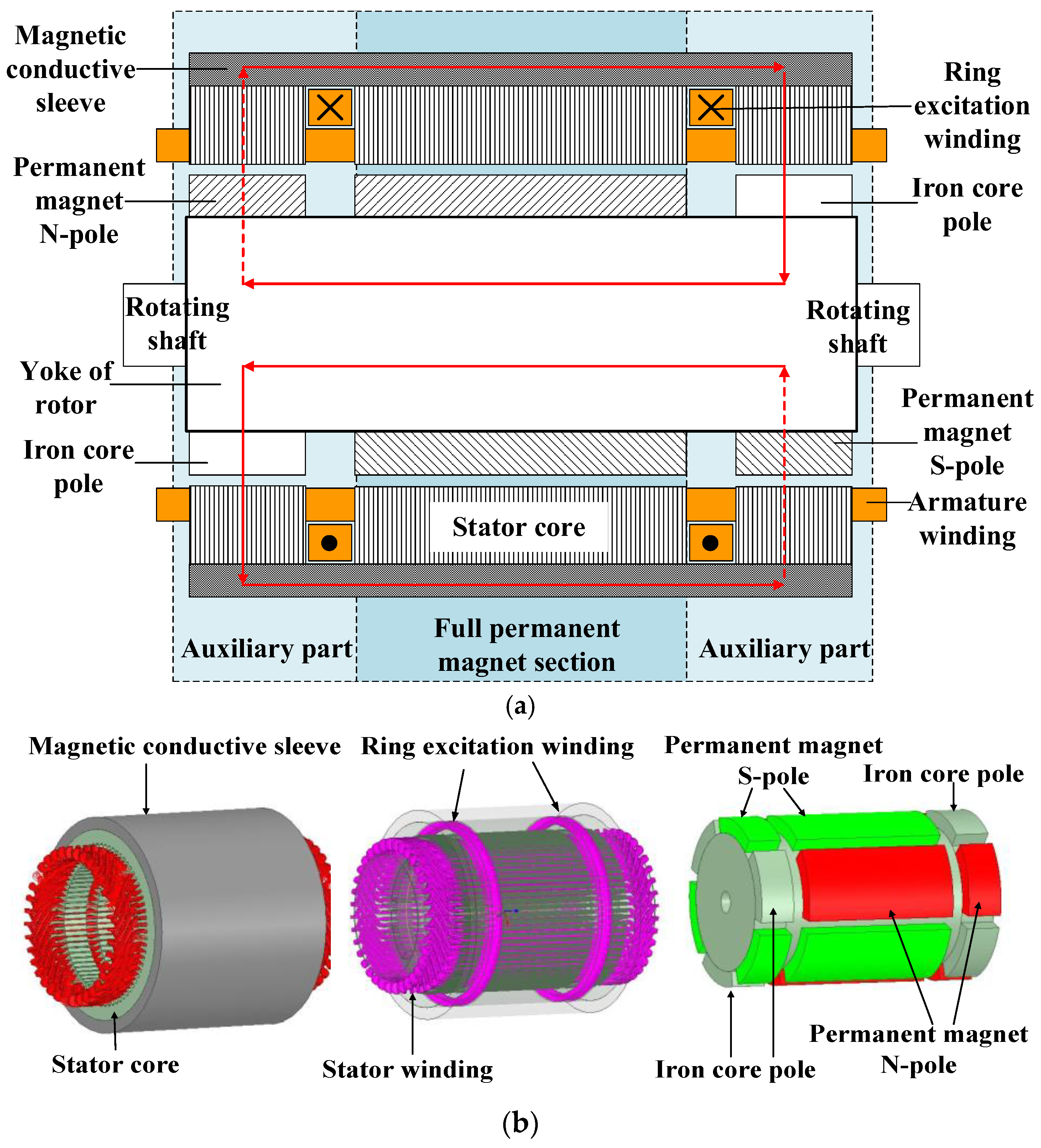
2.1. Basic Structure

The hybrid excitation generator of the double excitation winding is divided into a full permanent magnet part and an auxiliary part along the axial direction. The full permanent magnet part is located in the middle of the motor, and the auxiliary part is located on both sides of the motor, as shown in Figure 1. Among them, the red line represents the path through which the magnetic flux flows and the dotted line indicates that the magnetic flux needs to pass through the path with the minimum magnetic resistance, causing bending.

The stator core of the motor is composed of silicon steel stacks of the same structure, which are divided into three sections along the axial direction, namely the full permanent magnet part and the two symmetrical auxiliary parts. Two sets of coaxial and symmetrical ring excitation coils are arranged in the stator core. The two coils are connected in series to form the electric excitation winding, providing the axial magnetic circuit under the action of the external DC power supply, and the lower edge of the stator excitation winding is insulated and isolated from the armature winding. The armature winding passes through three stator cores, running through the entire axial length of the motor. In addition to the stator core, there is also a magnetic conductive sleeve to provide the motor with the axial magnetic circuit generated by the electric excitation. The motor structure of the full permanent magnet part is the same as that of the traditional surface of the attached permanent magnet motor and the rotor part; the motor structure of the auxiliary part is the same as that of the alternating pole permanent magnet motor, with both the core pole and the permanent magnet pole on the rotor. The rotor part corresponding to the two groups of annular excitation windings on the stator separates the full permanent magnet part from the auxiliary part with the diaphragm block to reduce the magnetic leakage of the permanent magnet.

2.2. Working Principle

The axial flux generated by the two sets of annular excitation windings is converted into radial flux on both sides. The magnetic flux path of the direct current excitation winding is rotor corepole-air-gap-stator core-conductive sleeve (axial)-stator core-air-gap on the other side of the rotor core-pole rotor yoke (axial)-rotor core pole, from which the electric excitation flux can be realized from axial to radial transition. As shown in Figure 1a, the red line represents the flow path of the magnetic flux generated by the ring excitation winding, which only flows through the iron core pole and not through the permanent magnet. Use solid lines to represent the actual flow path and dashed lines to represent the flow path that is curved and bypassed.

When the electric excitation winding is energized, the magnetic motive force generated by the two groups of annular excitation windings has the opposite effect on the middle full permanent magnet part, and they can cancel each other. When the excitation current is adjusted, the air-gap magnetic density of the full permanent magnetic part remains unchanged. In the auxiliary part, because the magnetic resistance of the permanent magnet pole is greater than the core pole, the electric excitation along the radial magnetic mainly primarily passes through the core pole, not through the permanent magnet pole; therefore, when adjusting the excitation current, the auxiliary part of the permanent magnet pole air-gap magnetic density change is very small, and the auxiliary part of the core pole of the air-gap magnetic density changes obviously and can thus make the total adjustment of each pole. When the axial magnetic flux generated by the excitation winding is converted into radial magnetic flux, the terminal voltage generated by the motor is the minimum; the terminal voltage generated by the motor increases when the excitation current gradually increases; when the terminal voltage of the motor increases in the opposite direction, the terminal voltage reaches the maximum value. Thus, the motor voltage can be adjusted.

From the above analysis, it can be concluded that when the generator voltage reaches the minimum, the motor is in the no-load state, and its structure can be basically equivalent to the table-stick permanent magnet generator. In the following study, analytical calculations were performed based on the above conclusions.

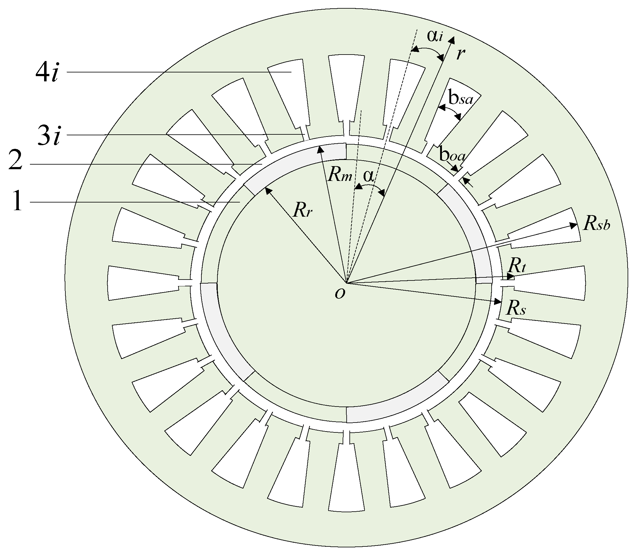
3. Accurate Subdomain Model Analysis

3.1. Basic Assumptions

Ignoring the effect of the motor end effect, the motor magnetic field distribution is reduced to a two-dimensional field problem; that is, the magnetic field is uniformly distributed along the axial direction of the motor. In order to facilitate the establishment of a two-dimensional magnetic field analytical model of the full permanent magnet motor, the magnetic field solution domain of the motor is usually divided into boundary rules and continuous solvable magnetic field subregions, and the following assumptions need to be made:

(1)

The magnetic permeability of the stator and rotor core is infinite;

(2)

The demagnetization curve of the permanent magnet material is linear;

(3)

Ignoring the conductance effect and eddy current effect of ferromagnetic materials.

Based on the above assumptions, ignoring the conductance effect and the vortex effect, the magnetic field of the permanent magnet motor is mainly generated by the steady constant current and the permanent magnet, which is a constant magnetic field. Because the permeability of ferromagnetic materials is infinite, the magnetic field of the permanent magnet motor can be divided into three areas: the magnetization area (permanent magnet area), the current carrying area (stator winding area), and the passive area (air area). In a two-dimensional magnetic field analysis, the magnetic vector potential has only the axial component Az. In different material media, Equation (1) can be simplified separately:

$${\nabla }^2\mathit{A}-\mu \sigma \frac{\partial \mathit{A}}{\partial t}=-\nabla \times {\mathit{B}}_{\mathit{r}}+\mu \sigma \nabla \phi$$

(1)

Equation (1) is the general form of the electromagnetic field diffusion equation satisfied by the vector magnetic bit $\mathit{A}$ and the scalar potential $\phi$ in the medium, which can be simplified according to the material properties and assumptions of the distribution region of the electromagnetic field.

In the permanent magnet region, the residual magnetic density can be represented as ${\mathit{B}}_{\mathit{r}}={\mu }_0\mathit{M}$. ${\mu }_0$ is the air magnetic permeability. $\mathit{M}$ is the residual magnetization, which can be decomposed into the radial and tangential components $M_r$, $M_{\alpha }$. In the 2D polar frame, $r$ and $\alpha$ indicate the radial and tangential positions, respectively. Formula (1) can be reduced to the following:

$$\frac{{\partial }^2{A}_z}{\partial r^2}+\frac{1}{r}\frac{\partial A_z}{\partial r}+\frac{1}{r^2}\frac{{\partial }^2{A}_z}{\partial {\alpha }^2}=-\frac{{\mu }_0}{r}(M_{\alpha }-\frac{\partial M_r}{\partial \alpha })$$

(2)

In the carrier region, the current density is in the winding region. Formula (1) can be reduced to $J_s={\mu }_0\sigma \nabla \phi$.

$$\frac{{\partial }^2{A}_z}{\partial r^2}+\frac{1}{r}\frac{\partial A_z}{\partial r}+\frac{1}{r^2}\frac{{\partial }^2{A}_z}{\partial {\alpha }^2}=-{\mu }_0{J}_s$$

(3)

In passive regions, Equation (1) can be reduced to the following:

$$\frac{{\partial }^2{A}_z}{\partial r^2}+\frac{1}{r}\frac{\partial A_z}{\partial r}+\frac{1}{r^2}\frac{{\partial }^2{A}_z}{\partial {\alpha }^2}=0$$

(4)

Equations (2) and (3) are Poisson equations, and Equation (4) is a Laplace equation. The general solution of the above equation can be found directly by separating the variable method, and then, the magnetic field boundary condition is applied to find the solution, that is, the solution of the vector magnetic field in the two-dimensional magnetic field distribution model.

There are three types of boundary conditions in a 2D constant magnetic field: periodic boundary conditions, Newman boundary conditions, and continuous boundary conditions. Periodic boundary conditions are the boundary conditions often used to calculate periodic symmetric structures. The Newman boundary condition in the magnetic field analysis usually refers to the tangential component of the magnetic field strength at the partition interface with the core when the core magnetic conductivity is infinite. The continuous boundary condition of a two-dimensional magnetic field mainly refers to the continuity of the axial vector magnetic bit, the scalar magnetic bit, the radial component of the magnetic density, and the tangential component of the magnetic field strength at the two magnetic field interfaces.

The radial and tangential components of the magnetic density and the magnetic vector potential are related to the following:

$$B_r=\frac{1}{r}\frac{\partial A_z}{\partial \alpha }$$

(5)

$$B_{\alpha }=-\frac{\partial A_{zj}}{\partial r}$$

(6)

The cross-section of the permanent magnet motor is shown in Figure 2.

In Figure 2, R_r, R_m, R_s, R_t, and R_sb represent the outer radius of the rotor core, the permanent magnet radius, the stator core radius, the groove top radius, and the groove bottom arc radius; boa and bsa are the groove width and groove width angle, respectively.

According to the geometry of the motor magnetic field solution region and the magnetic field region category, the motor magnetic field solution domain can be divided into four subdomains: 1—permanent, 2—air-gap subdomain, 3i-i (i = 1, 2, 3…)—stator slot hole domain, and 4i-i—stator slot subdomain. The axial components of the corresponding regions are expressed by A_z1, A_z2, A_z3i, and A_z4i.

The permanent magnet motor structure is flexible, and the magnetic circuit is complex and changeable; in order to improve the universality of the permanent magnet motor field analytical model, in the present paper, we put forward permanent magnetic field analytical modeling ideas; according to the structure of the permanent magnet motor, the motor field solution domain is divided into the rotor domain, stator domain, and air-gap domain, and strong independence and portability were established with the good modular subdomain magnetic field analytical model. Among them, the stator domain contains two magnetic field subdomains, the stator slot hole domain and the stator slot subdomain.

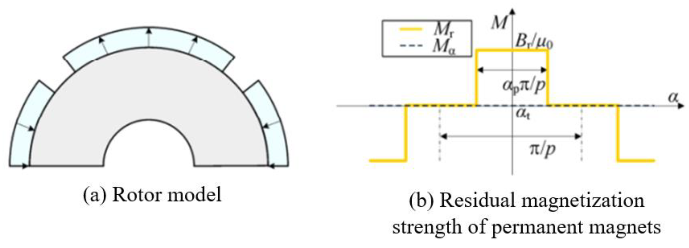
3.2. Analytic Model of the Magnetic Field in the Rotor Domain

The rotor magnetic circuit of a permanent magnet motor is mainly composed of a rotor core and a permanent magnet. The permanent magnet of the table-type permanent magnet motor is attached to the surface of the rotor. Assuming that the core permeability is infinite, the air between the poles of the rotor permanent magnet can be equivalent to the permanent magnet with a residual magnetization strength of 0. The problem of solving the magnetic field in the rotor domain can be converted into the magnetic field calculation of the permanent magnet subdomain (including the air part between the rotor poles).

The initial position angle of the rotor of the permanent magnet motor is set as ${\alpha }_0$. When the motor rotor speed is ${\omega }_r$, the angular difference between the rotor coordinate system and the stator coordinate system is ${\alpha }_t={\omega }_{r}t+{\alpha }_0$. Using the stator stationary coordinate system as a reference, the radial $M_r$ and tangential $M_{\alpha }$ components of the magnet magnetization can be decomposed into Fourier series on the circumference, as follows:

$$\begin{array}{l}{M}_r={\displaystyle \sum _k{M}_{rk}\cos (k\alpha -k{\alpha }_t)}={\displaystyle \sum _k{M}_{rck}\cos k\alpha +M_{rsk}\sin k\alpha }\\ M_{\alpha }={\displaystyle \sum _k{M}_{\alpha k}\sin (k\alpha -k{\alpha }_t)}={\displaystyle \sum _k{M}_{\alpha ck}\cos k\alpha +M_{\alpha sk}\sin k\alpha }\end{array}$$

(7)

where $M_{rck}=M_{rk}\cos (k{\alpha }_t)$, $M_{rsk}=M_{rk}\sin (k{\alpha }_t)$, $M_{\alpha ck}=-M_{\alpha k}\sin (k{\alpha }_t)$, $M_{\alpha sk}=M_{\alpha k}\cos (k{\alpha }_t)$; $k$ is the harmonic coefficient; $M_{rk}$ and $M_{\alpha k}$ are the Fourier coefficients of the radial and tangential components $M_r$ and $M_{\alpha }$ of the residual magnetization, respectively.

The main charging modes of the permanent magnet rotors are radial magnetism, parallel magnetism, and Halbach magnetism. The polar log is p, and the polar arc coefficient is ${\alpha }_p$. The residual flux density is a permanent magnet of $B_r$. In the present study, the main case is considered. The rotor model and the residual magnetization of the permanent magnet are shown in Figure 3, and the Fourier series expression of the residual magnetization of the permanent magnet is, respectively:

$$\begin{array}{l}{M}_{rk}=\frac{4p{B}_r}{k\pi {\mu }_0}\sin \frac{k\pi {\alpha }_p}{2p}, k/p=1,3,5\dots \\ M_{\alpha k}=0, k/p=1,3,5\dots \end{array}$$

(8)

The vector magnetic bit $A_{z1}$ of the permanent magnet subdomain satisfies the Poisson Equation (2), using the separation variable method and applying the periodic boundary condition of the rotating motor:

$$A_{z1}={\displaystyle \sum _k[A_{1k}{(\frac{r}{R_m})}^k+B_{1k}{(\frac{r}{R_r})}^{-k}]}\cos \left(k\alpha \right)+{\displaystyle \sum _k[C_{1k}{(\frac{r}{R_m})}^k+D_{1k}{(\frac{r}{R_r})}^{-k}]}\sin \left(k\alpha \right)+A_{p1}$$

(9)

where $A_{1k},B_{1k},C_{1k},D_{1k}$ is the undetermined coefficient and $A_{p1}$ is the special solution.

k ≠ 1, then

$$A_{p1}={\mu }_{0}r{\displaystyle \sum _k\frac{1}{k^2-1}\left[\left(M_{\alpha ck}-k{M}_{rsk}\right)\cos (k\alpha )+\left(M_{\alpha sk}+k{M}_{rck}\right)\sin (k\alpha )\right]}$$

(10)

k = 1, then

$$A_{p1}=-\frac{{\mu }_{0}r\ln r}{2}\left[\left(M_{\alpha c1}-M_{rs1}\right)\cos \alpha +\left(M_{\alpha s1}+M_{rc1}\right)\sin \alpha \right]$$

(11)

In combination with Formula (6), the tangential magnetic density expression in the permanent magnet is as follows:

$$\begin{array}{ll}{B}_{\alpha 1}& =-\frac{k}{r}{\displaystyle \sum _k[A_{1k}{(\frac{r}{R_m})}^k-B_{1k}{(\frac{r}{R_r})}^{-k}]}\cos \left(k\alpha \right)-\frac{k}{r}{\displaystyle \sum _k[C_{1k}{(\frac{r}{R_m})}^k-D_{1k}{(\frac{r}{R_r})}^{-k}]}\sin \left(k\alpha \right)\\ & -{\mu }_0{\displaystyle \sum _k\frac{1}{k^2-1}\left[\left(M_{\alpha ck}-k{M}_{rsk}\right)\sin (k\alpha )+\left(M_{\alpha sk}+k{M}_{rck}\right)\cos (k\alpha )\right]}\end{array}$$

(12)

On the surface of the rotor core, the boundary condition satisfying the tangential magnetic field strength is zero, with

$$H_{\alpha 1}{|}_{r=R_m}=\frac{B_{\alpha 1}{|}_{r=R_m}}{{\mu }_0{\mu }_r}-\frac{M_{\alpha }{|}_{r=R_m}}{{\mu }_r}=0$$

(13)

The expression of the residual magnetization in the permanent magnet:

$$B_{1k}=A_{1k}{G}_{1k}+\frac{{\mu }_0{R}_r}{k^2-1}(k{M}_{\alpha ck}-M_{rsk})$$

(14)

$$D_{1k}=C_{1k}{G}_{1k}+\frac{{\mu }_0{R}_r}{k^2-1}(k{M}_{\alpha sk}+M_{rck})$$

(15)

In the formula, $G_{1k}={(R_r/R_m)}^k$.

Thus, the vector magnetic bit expression in the permanent magnet can be reduced to the following:

$$\begin{array}{ll}{A}_{z1}& ={\displaystyle \sum _k{A}_{1k}[{(\frac{r}{R_m})}^k+G_{1k}{(\frac{r}{R_r})}^{-k}]}\cos \left(k\alpha \right)+{\displaystyle \sum _k{C}_{1k}[{(\frac{r}{R_m})}^k+G_{1k}{(\frac{r}{R_r})}^{-k}]}\sin \left(k\alpha \right)\\ & +{\mu }_0{\displaystyle \sum _k\frac{1}{k^2-1}\{[k{R}_r{(\frac{r}{R_r})}^{-k}+r]M_{\alpha ck}-[R_r{(\frac{r}{R_r})}^{-k}+kr]M_{rsk}\}\cos (k\alpha )}\\ & +{\mu }_0{\displaystyle \sum _k\frac{1}{k^2-1}\{[k{R}_r{(\frac{r}{R_r})}^{-k}+r]M_{\alpha sk}+[R_r{(\frac{r}{R_r})}^{-k}+kr]M_{rck}\}\sin (k\alpha )}\end{array}$$

(16)

In the permanent magnet subdomain, the flux density radial component $B_{r1}$ and the tangential component $B_{\alpha 1}$ are as follows:

$$\begin{array}{ll}\hfill B_{r1}& =-\frac{1}{r}{\displaystyle \sum _{k}k{A}_{1k}[{(\frac{r}{R_m})}^k+G_{1k}{(\frac{r}{R_r})}^{-k}]\sin (k\alpha )}\\ & +\frac{1}{r}{\displaystyle \sum _{k}k{C}_{1k}[{(\frac{r}{R_m})}^k+G_{1k}{(\frac{r}{R_r})}^{-k}]\cos (k\alpha )}\\ & -{\mu }_0{\displaystyle \sum _k\frac{1}{k^2-1}\{[k{(\frac{r}{R_r})}^{-k-1}+1]M_{\alpha ck}-[k{(\frac{r}{R_r})}^{-k-1}+k]M_{rsk}\}}\sin (k\alpha )\\ & +{\mu }_0{\displaystyle \sum _k\frac{1}{k^2-1}\{[k{(\frac{r}{R_r})}^{-k-1}+1]M_{\alpha sk}+[k{(\frac{r}{R_r})}^{-k-1}+k]M_{rck}\}}\cos (k\alpha )\\ H_{r1}& =\frac{B_{r1}}{{\mu }_0{\mu }_{\mathrm{r}}}\end{array}$$

(17)

$$\begin{array}{ll}{B}_{\alpha 1}& =-\frac{1}{r}{\displaystyle \sum _{k}k{A}_{1k}[{(\frac{r}{R_m})}^k-G_{1k}{(\frac{r}{R_r})}^{-k}]\cos (k\alpha )}\\ & -\frac{1}{r}{\displaystyle \sum _{k}k{C}_{1k}[{(\frac{r}{R_m})}^k-G_{1k}{(\frac{r}{R_r})}^{-k}]\sin (k\alpha )}\\ & +{\mu }_0{\displaystyle \sum _k\frac{1}{k^2-1}\{[k^2{(\frac{r}{R_r})}^{-k-1}-1]M_{\alpha ck}-[k{(\frac{r}{R_r})}^{-k-1}-k]M_{rsk}\}}\cos (k\alpha )\\ & +{\mu }_0{\displaystyle \sum _k\frac{1}{k^2-1}\{[k^2{(\frac{r}{R_r})}^{-k-1}-1]M_{\alpha sk}+[k{(\frac{r}{R_r})}^{-k-1}-k]M_{rck}\}}\sin (k\alpha )\\ H_{\alpha 1}& =\frac{B_{\alpha 1}}{{\mu }_0{\mu }_{\mathrm{r}}}\end{array}$$

(18)

3.3. Analytic Model of the Magnetic Field in the Stator Domain

The stator domain contains two magnetic field subdomains, the stator groove hole domain and the stator groove subdomain. The influence on the motor caused by the groove opening can be considered. The groove opening and winding distribution are shown in Figure 4 below.

3.3.1. The Stator Slot Sub-Domain

When the permanent magnet motor adopts a concentrated winding, the current density distribution is shown in Figure 4. The Fourier series of the stator slot interval can be obtained, as follows:

$$J_i=J_{i0}+{\displaystyle \sum _m{J}_{im}\cos [F_m(\alpha +b_{sa}/2-{\alpha }_i)]}$$

(19)

where $F_m=m\pi /b_{sa}, m=1,2,3,\dots$ is the number of magnetic field harmonics in the stator slot area:

$$J_{im}=2[J_{i1}+J_{i2}\cos (m\pi )]\sin (m\pi d/b_{sa})/(m\pi ) \mathrm{and} J_{i0}=(J_{i1}+J_{i2})d/b_{sa}.$$

where d is the radian corresponding to the area occupied by each layer of winding in the slot; $J_{i1}\mathrm{and}{J}_{i2}$ are the current density of the left and right layers of the winding in the i-th groove.

The stator groove region is the current load area when the motor is running, and the passive region is when the stator winding is open. The stator winding can also be regarded as if the current density of the carrier area is 0. In order to facilitate the establishment of a unified model, the stator groove region is modeled according to the current carrying area, and the appropriate amount of magnetic bits satisfies the Poisson equation constraint in Formula (3).

Using the separation variable method and applying the boundary condition of the zero value of the radial component of the strength of the magnetic field in the stator groove subdomain:

$$A_{z4i}={\displaystyle \sum _m{D}_{4im}[G_{4m}{(\frac{r}{R_t})}^{F_m}+{(\frac{r}{R_{sb}})}^{-F_m}]\cos [F_m(\alpha +b_{sa}/2-{\alpha }_i)]}+A_{4ip}$$

(20)

where $D_{4im}$ is the pending coefficient; $A_{4ip}$ is the specific solution; and $G_{4m}={(R_t/R_{sb})}^{F_m}$.

For concentrated windings with a double-layer distribution on the left and right sides, there is:

$$A_{4ip}={\displaystyle \sum _m\frac{{\mu }_0{J}_{im}}{F_m^2-4}[r^2-\frac{2}{F_m}{R}_{sb}^2{(\frac{r}{R_{sb}})}^{F_m}]\cos [F_m(\alpha +\frac{b_{sa}}{2}-{\alpha }_i)]}+\frac{{\mu }_0{J}_{i0}}{4}(2R_{sb}^2\ln r-r^2)+Q_{4i}$$

(21)

where $Q_{4i}$ is the undetermined coefficient.

3.3.2. Stator Slot Hole Field

The stator slot region is passive, and its magnetic vector potential satisfies the Laplace equation constraint in Equation (4). Using the separation variable method and applying the boundary condition on the two sides of the groove, the expression of the vector magnetic field is zero:

$$A_{z3i}={\displaystyle \sum _n[C_{3in}{(\frac{r}{R_t})}^{E_n}+D_{3in}{(\frac{r}{R_s})}^{-E_n}]\cos [E_n(\alpha +b_{oa}/2-{\alpha }_i)]}+D_i\ln r+Q_{3i}$$

(22)

where $C_{3in},D_{3in},D_i,Q_{3i}$ is the undetermined coefficient.

Combined with Equation (6), the tangential magnetic density at the groove can be obtained:

$$B_{\alpha 3i}{|}_{r=R_t}=-\frac{1}{r}{\displaystyle \sum _n{E}_n(C_{3in}{(\frac{r}{R_t})}^{E_n}-D_{3in}{(\frac{r}{R_s})}^{-E_n})\cos [E_n(\alpha +b_{oa}/2-{\alpha }_i)]}-\frac{D_i}{r}$$

(23)

The vector magnetic bit is continuous and satisfied at the division interface:

$$A_{z3i}{|}_{r=R_t}=A_{z4i}{|}_{r=R_t}$$

(24)

When using a centralized winding with double-layer distribution on both sides, expand the vector magnetic potential of $A_{z4i}{|}_{r=R_t}$ at the slot into intervals $[{\alpha }_i-b_{oa}/2, {\alpha }_i+b_{oa}/2]$ Fourier series:

$$\begin{array}{ll}{A}_{z4i}{|}_{r=R_t}& ={\displaystyle \sum _n{\displaystyle \sum _m[D_{4im}(G_{4m}^2+1)+{\mu }_0\frac{J_{im}}{F_m^2-4}(R_t^2-\frac{2}{F_m}{R}_{sb}^2{G}_{4m})}]{\zeta }_i(m,n)}\\ & \times \cos [E_n(\alpha +\frac{b_{oa}}{2}-{\alpha }_i)]+{\mu }_0{J}_{i0}(2R_{sb}^2\ln R_t-R_t^2)/4+Q_{4i}\\ & +{\displaystyle \sum _m[D_{4im}(G_{4m}^2+1)+{\mu }_0\frac{J_{im}}{F_m^2-4}(R_t^2-\frac{2}{F_m}{R}_{sb}^2{G}_{4m})}]{\zeta }_{i0}(m)\end{array}$$

(25)

In the formula,

$${\zeta }_i(m,n)=\frac{-2F_m[\cos (n\pi )\sin (F_m{b}_{sa}/2+F_m{b}_{oa}/2))-\sin (F_m{b}_{sa}/2-F_m{b}_{oa}/2)]}{b_{oa}(E_n^2-F_m^2)};$$

$${\zeta }_{i0}(m)=2b_{sa}\cos (m\pi /2)\sin (F_m{b}_{oa}/2)/(m\pi b_{oa});$$

The following can be obtained from Equations (22), (24) and (25)

$$C_{3in}+D_{3in}{G}_{3n}={\displaystyle \sum _m[D_{4im}(G_{4m}^2+1)+{\mu }_0\frac{J_{im}}{F_m^2-4}(R_t^2-\frac{2}{F_m}{R}_{sb}^2{G}_{4m})]{\zeta }_i(m,n)}$$

(26)

$$\begin{array}{ll}{Q}_{4i}& =-{\displaystyle \sum _m[D_{4im}(G_{4m}^2+1)+{\mu }_0\frac{J_{im}}{F_m^2-4}(R_t^2-\frac{2}{F_m}{R}_{sb}^2{G}_{4m})]{\zeta }_{i0}(m)}\\ & {+\mathrm{D}}_i\ln R_t+Q_{3i}-\frac{{\mu }_0{J}_{i0}}{4}(2R_{sb}^2\ln R_t-R_t^2)\end{array}$$

(27)

In the formula, $G_{3n}={(R_s/R_t)}^{E_n}$.

The tangential magnetic field strength at the interface between the stator slot subdomain and the slot subdomain has continuity, satisfying the following:

$$H_{\alpha 3i}{|}_{r=R_t}=H_{\alpha 4i}{|}_{r=R_t}$$

(28)

Combined with the relationship between magnetic density and magnetic field intensity in the air medium, Equation (28) can be equivalent to the following:

$$B_{\alpha 3i}{|}_{r=R_t}=B_{\alpha 4i}{|}_{r=R_t}$$

(29)

Break down Equation (23) into the Fourier series on the interval $[{\alpha }_i-b_{sa}/2, {\alpha }_i+b_{sa}/2]$,

$$\begin{array}{l}{B}_{\alpha 3i}{|}_{r=R_t}=-{\displaystyle \sum _m[{\displaystyle \sum _n{E}_n(C_{3in}-D_{3in}{G}_{3n}){\gamma }_i(m,n)+D_i}{\gamma }_{i0}(m)]}\\ \times \cos [E_n(\alpha +b_{oa}/2-{\alpha }_i)]/R_t-D_i{b}_{oa}/(R_t{b}_{sa})\end{array}$$

(30)

In the formula, ${\gamma }_i(m,n)=b_{oa}{\zeta }_i(m,n)/b_{sa}$ and ${\gamma }_{i0}(m)=2b_{oa}{\zeta }_{i0}(m)/b_{sa}$.

When using a concentrated winding with a left and right double-layer distribution,

$$\begin{array}{l}{B}_{\alpha 4i}{|}_{r=R_t}=-\frac{1}{R_t}{\displaystyle \sum _m[F_m{D}_{4im}(G_{4m}^2-1)+\frac{2{\mu }_0{J}_{im}}{F_m^2-4}(R_t^2-R_{sb}^2{G}_{4m})]}\\ \times \cos [F_m(\alpha +b_{sa}/2-{\alpha }_i)]-{\mu }_0{J}_{i0}(R_{sb}^2-R_t^2)/(2R_t)\end{array}$$

(31)

The following can be obtained from Equations (29)–(31):

$${\displaystyle \sum _n{E}_n(C_{3in}-D_{3in}{G}_{3n}){\gamma }_i+D_i{\gamma }_{io}(m)}=F_m{D}_{4im}(G_{4m}^2-1)+\frac{2{\mu }_0{J}_{im}}{F_m^2-4}(R_t^2-R_{sb}^2{G}_{4m})$$

(32)

$$D_i=b_{sa}{\mu }_0{J}_{i0}(R_{sb}^2-R_t^2)/(2b_{oa})$$

(33)

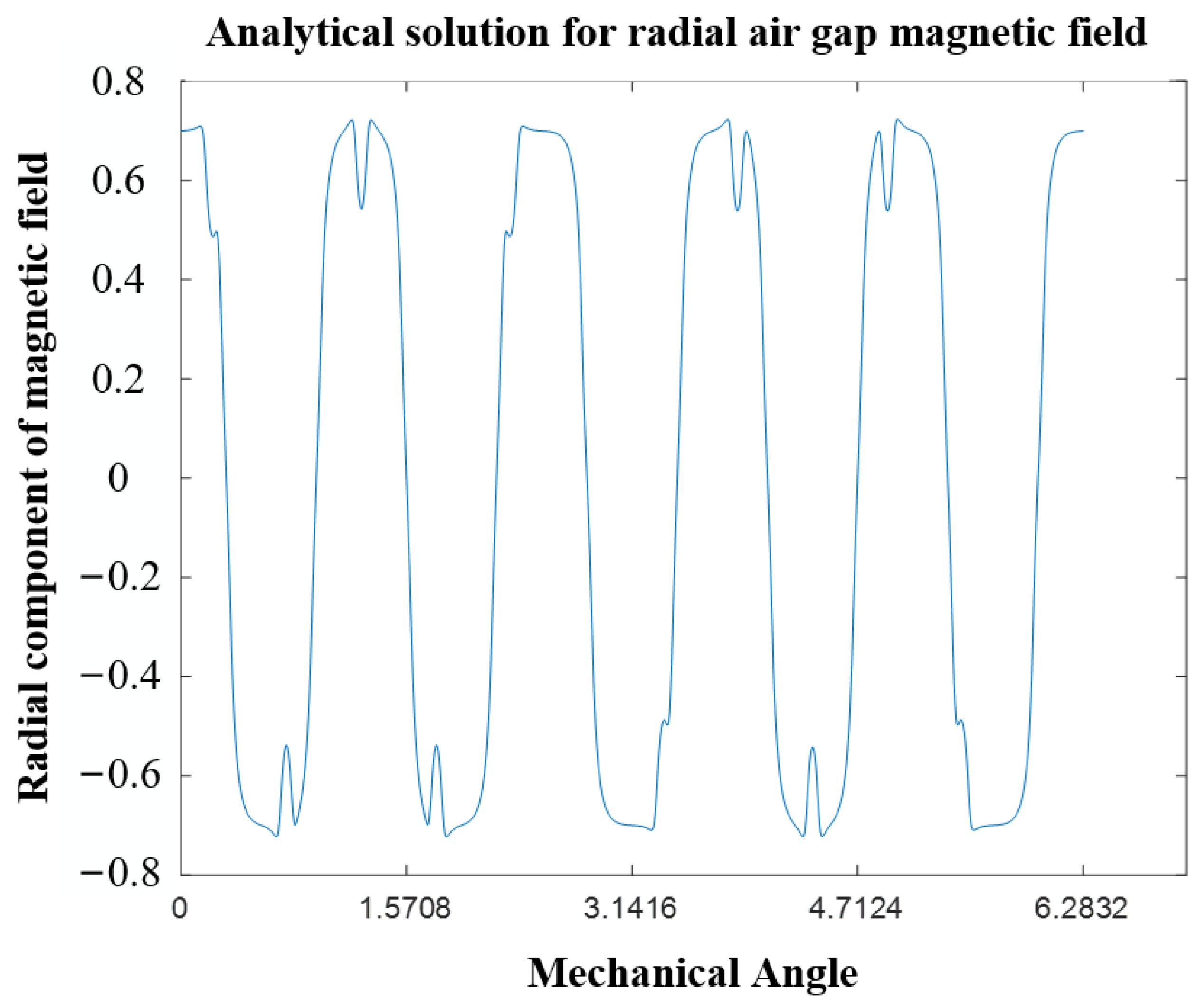
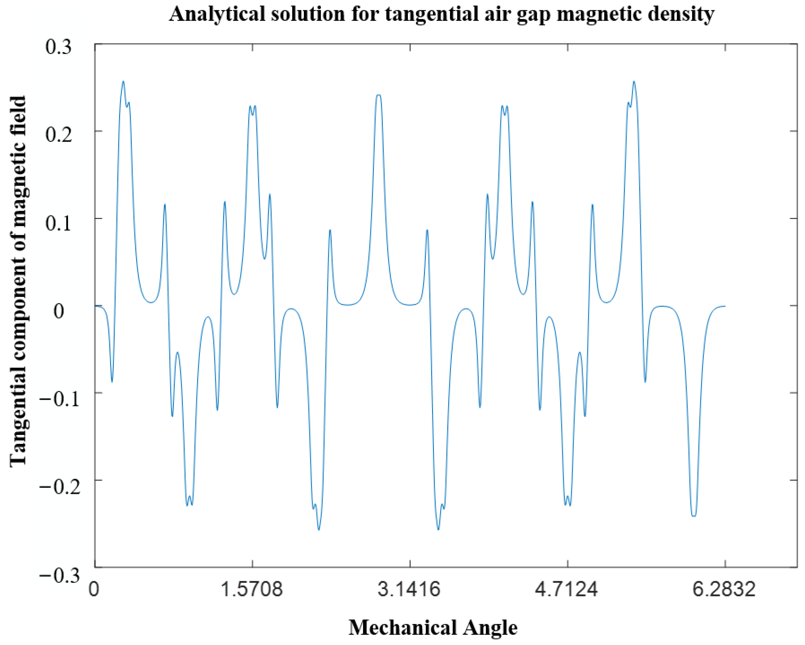
3.4. Analytic Model of the Magnetic Field in the Air-Gap Domain

The air gap is the hub of the coupling and interaction between the rotor excitation magnetic field and the stator armature reaction magnetic field. When the rotor permanent magnet is a regular concentric tile structure, the air-gap region in the permanent magnetic field analytical model is a circular area. The air-gap region is a uniformly distributed air medium that belongs to the passive region and satisfies the constraint of Equation (4). Using the separation variable method, the analytical expression of the vector:

$$A_{z2}={\displaystyle \sum _k[A_{2k}{(\frac{r}{R_s})}^k+B_{2k}{(\frac{r}{R_m})}^{-k}]}\cos \left(k\alpha \right)+{\displaystyle \sum _k[C_{2k}{(\frac{r}{R_s})}^k+D_{2k}{(\frac{r}{R_m})}^{-k}]}\sin \left(k\alpha \right)$$

(34)

where $A_{2k},B_{2k},C_{2k},D_{2k}$ for the set coefficient.

The magnetic dense radial component $B_{r2}$ and tangential component $B_{\alpha 2}$ are obtained from Equation (5) and Equation (6), respectively:

$$B_{r2}=-{\displaystyle \sum _k\frac{k}{r}[A_{2k}{(\frac{r}{R_s})}^k+B_{2k}{(\frac{r}{R_m})}^{-k}]\sin (k\alpha )}+{\displaystyle \sum _k\frac{k}{r}[C_{2k}{(\frac{r}{R_s})}^k+D_{2k}{(\frac{r}{R_m})}^{-k}]\cos (k\alpha )}$$

(35)

$$B_{\alpha 2}=-{\displaystyle \sum _k\frac{k}{r}[A_{2k}{(\frac{r}{R_s})}^k-B_{2k}{(\frac{r}{R_m})}^{-k}]\cos (k\alpha )}-{\displaystyle \sum _k\frac{k}{r}[C_{2k}{(\frac{r}{R_s})}^k-D_{2k}{(\frac{r}{R_m})}^{-k}]\sin (k\alpha )}$$

(36)

$B={\mu }_{0}H$ is satisfied between the magnetic density and the magnetic field intensity in the air medium, and the magnetic field strength in the air gap can be obtained as follows:

$$H_{r2}=-\frac{1}{{\mu }_{0}r}{\displaystyle \sum _{k}k[A_{2k}{(\frac{r}{R_s})}^k+B_{2k}{(\frac{r}{R_m})}^{-k}]\sin (k\alpha )}+\frac{1}{{\mu }_{0}r}{\displaystyle \sum _{k}k[C_{2k}{(\frac{r}{R_s})}^k+D_{2k}{(\frac{r}{R_m})}^{-k}]\cos (k\alpha )}$$

(37)

$$H_{\alpha 2}=-\frac{1}{{\mu }_{0}r}{\displaystyle \sum _{k}k[A_{2k}{(\frac{r}{R_s})}^k-B_{2k}{(\frac{r}{R_m})}^{-k}]\cos (k\alpha )}-\frac{1}{{\mu }_{0}r}{\displaystyle \sum _{k}k[(C_{2k}{(\frac{r}{R_s})}^k-D_{2k}{(\frac{r}{R_m})}^{-k}]\sin (k\alpha )}$$

(38)

According to the motor structure, it is divided into three regions: the rotor domain, the stator domain (including the groove subdomain and groove hole domain), and the air-gap domain, and the magnetic field analytical model of each region is respectively established.

3.5. Boundary Conditions

Using the air-gap boundary condition, it is possible to establish the constraint system of the undetermined coefficient in the analytical expression of the magnetic field in each region, solve the undetermined coefficient, and then obtain the expression of the vector magnetic field in each region. Furthermore, the analytical model was used to analyze the electromagnetic parameters and performance of the motor.

The motor stator armature reaction magnetic field is coupled with the rotor excitation magnetic field through the air gap. The inner and outer boundaries of the air gap are the division interfaces with the rotor and the stator, respectively. Two continuous boundary conditions for vector magnetic continuous and tangential magnetic field strength are satisfied at the division interface.

(1) The vector magnetic bit has continuity at the interface between the air gap and the rotor permanent magnet:

$$A_{z1}{|}_{r=R_m}=A_{z2}{|}_{r=R_m}$$

(39)

The combination of Equations (16), (34), and (39) can be obtained as follows:

$$A_{1k}(1+{G_{1k}}^2)+\frac{{\mu }_0}{k^2-1}[(R_{r}k{G}_{1k}+R_m)M_{\alpha ck}-(R_r{G}_{1k}+k{R}_m)M_{rsk}]=A_{2k}{G}_{2k}+B_{2k}$$

(40)

$$C_{1k}(1+{G_{1k}}^2)+\frac{{\mu }_0}{k^2-1}[(R_{r}k{G}_{1k}+R_m)M_{\alpha sk}+(R_r{G}_{1k}+k{R}_m)M_{rck}]=C_{2k}{G}_{2k}+D_{2k}$$

(41)

In the formula, $G_{2k}={(R_m/R_s)}^k$.

(2) The strength of the tangential magnetic field at the interface between the air gap and the rotor permanent magnet is continuous and satisfied:

$$H_{\alpha 1}{|}_{r=R_m}=H_{\alpha 2}{|}_{r=R_m}$$

(42)

The combination of Equations (18), (38), and (42) can be obtained:

$$A_{1k}(1-{G_{1k}}^2)+\frac{{\mu }_0}{k^2-1}[k(R_m-R_r{G}_{1k})M_{\alpha ck}-(R_m-R_r{G}_{1k})M_{rsk}]={\mu }_r(A_{2k}{G}_{2k}-B_{2k})$$

(43)

$$C_{1k}(1-{G_{1k}}^2)+\frac{{\mu }_0}{k^2-1}[k(R_m-R_r{G}_{1k})M_{\alpha sk}+(R_m-R_r{G}_{1k})M_{rck}]={\mu }_r(C_{2k}{G}_{2k}-D_{2k})$$

(44)

(3) The vector magnetic bit has continuity at the interface between the air gap and stator, and the vector magnetic bit of the air gap and slot meet:

$$A_{z2}{|}_{r=R_s}=A_{z3i}{|}_{r=R_s}$$

(45)

Combined with Equation (34), let $A_{z2}{|}_{r=R_s}$ expand into intervals $[{\alpha }_i-b_{oa}/2, {\alpha }_i+b_{oa}/2]$ at the slot on the Fourier series, as follows:

$$\begin{array}{l}{A}_{z2}{|}_{r=R_s}={\displaystyle \sum _k[(A_{2k}+B_{2k}{G}_{2k}){\sigma }_{i0}(k)+(C_{2k}+D_{2k}{G}_{2k}){\tau }_{i0}(k)]}\\ +{\displaystyle \sum _n{\displaystyle \sum _k[(A_{2k}+B_{2k}{G}_{2k}){\sigma }_i(n,k)+(C_{2k}+D_{2k}{G}_{2k}){\tau }_i(n,k)]}}\cdot {\cos [\mathrm{E}}_n(\alpha +b_{oa}/2-{\alpha }_i\left)\right]\end{array}$$

(46)

In the formula,

$${\sigma }_i(n,k)=-2k[\cos (n\pi )\sin (k{\alpha }_i+k{b}_{oa}/2)-\sin (k{\alpha }_i-k{b}_{oa}/2)]/[b_{oa}({E_n}^2-k^2)];$$

$${\tau }_i(n,k)=2k[\cos (n\pi )\cos (k{\alpha }_i+k{b}_{oa}/2)-\cos (k{\alpha }_i-k{b}_{oa}/2)]/[b_{oa}({E_n}^2-k^2)];$$

$${\sigma }_{i0}(k)=2\sin (k{b}_{oa}/2)\cos (k{\alpha }_i)/(k{b}_{oa});{\tau }_{i0}(k)=2\sin (k{b}_{oa}/2)\sin (k{\alpha }_i)/(k{b}_{oa})$$

The combination of Equations (22), (45), and (46) can be obtained:

$${\displaystyle \sum _k[(A_{2k}+B_{2k}{G}_{2k}){\sigma }_i(n,k)+(C_{2k}+D_{2k}{G}_{2k}){\tau }_i(n,k)]}=C_{3in}{G}_{3n}+D_{3in}$$

(47)

$$Q_{3i}={\displaystyle \sum _k[(A_{2k}+B_{2k}{G}_{2k}){\sigma }_{i0}(k)+(C_{2k}+D_{2k}{G}_{2k}){\tau }_{i0}(k)]}-D_i\ln R_s$$

(48)

(4) The continuity of the tangential magnetic field strength at the interface between the air gap and the stator, and the tangential magnetic field strength at the air gap and the groove is satisfied:

$$H_{2\alpha }{|}_{r=R_s}={\displaystyle \sum _i{H}_{3i\alpha }{|}_{r=R_s}}$$

(49)

Combined with the relationship between magnetic density and magnetic field intensity in the air medium, the above equation can be equivalent to the following:

$$B_{2\alpha }{|}_{r=R_s}={\displaystyle \sum _i{B}_{3i\alpha }{|}_{r=R_s}}$$

(50)

Combined with formula (23), it expands the tangential magnetic density at each slot as the Fourier series on [0, 2π]:

$$\begin{array}{l}{\displaystyle \sum _i{B}_{3i\alpha }{|}_{r=R_s}}=-\frac{1}{R_s}{\displaystyle \sum _k{\displaystyle \sum _i[{\displaystyle \sum _n{E}_n(C_{3in}{G}_{3n}-D_{3in}){\eta }_i(n,k)+D_i}{\eta }_{i0}(k)]\cos (k\alpha )}}\\ -\frac{1}{R_s}{\displaystyle \sum _k{\displaystyle \sum _i[{\displaystyle \sum _n{E}_n(C_{3in}{G}_{3n}-D_{3ijn}){\xi }_i(n,k)+D_i}{\xi }_{i0}(k)]\sin (k\alpha )}}\end{array}$$

(51)

In the formula,

$${\eta }_i(n,k)=b_{oa}{\sigma }_i(n,k)/(2\pi ); {\xi }_i(n,k)=b_{oa}{\tau }_i(n,k)/(2\pi );$$

$${\eta }_{i0}(k)=b_{oa}{\sigma }_{i0}(k)/\pi ; {\xi }_{i0}(k)=b_{oa}{\tau }_{i0}(k)/\pi$$

The above can be obtained from Equations (36), (50), and (51):

$$k(A_{2k}-B_{2k}{G}_{2k})={\displaystyle \sum _i{\displaystyle \sum _n{E}_n(C_{3in}{G}_{3n}-D_{3in})}{\eta }_i(n,k)}+{\displaystyle \sum _i{D}_i{\eta }_{i0}(k)}$$

(52)

$$k(C_{2k}-D_{2k}{G}_{2k})={\displaystyle \sum _i{\displaystyle \sum _n{E}_n(C_{3in}{G}_{3n}-D_{3in})}{\xi }_i(n,k)}+{\displaystyle \sum _i{D}_i{\xi }_{i0}(k)}$$

(53)

3.6. Equation Solution and Correlation Coefficient

When the permanent magnet motor adopts the concentrated winding of the left and right double layer distribution, the joint vertical is as follows: Equations (26), (32), (40), (41), (43), (44), (47), (52) and (53).

The final matrix form can be simply expressed as $\mathbf{A}\mathbf{X}=Y$ in Equation (54). The specific expressions of each element in the matrix are shown in Appendix A.

$$\left[\begin{array}{ccccccccc}{K}_{11}& 0& K_{13}& K_{14}& 0& 0& 0& 0& 0\\ 0& K_{22}& 0& 0& K_{25}& K_{26}& 0& 0& 0\\ K_{31}& 0& K_{33}& K_{34}& 0& 0& 0& 0& 0\\ 0& K_{42}& 0& 0& K_{45}& K_{46}& 0& 0& 0\\ 0& 0& K_{53}& K_{54}& 0& 0& K_{57}& K_{58}& 0\\ 0& 0& 0& 0& K_{65}& K_{66}& K_{67}& K_{68}& 0\\ 0& 0& K_{73}& K_{74}& K_{75}& K_{76}& K_{77}& K_{78}& 0\\ 0& 0& 0& 0& 0& 0& K_{87}& K_{88}& K_{89}\\ 0& 0& 0& 0& 0& 0& K_{97}& K_{98}& K_{99}\end{array}\right]\left[\begin{array}{c}{A}_{1k}\\ C_{1k}\\ A_{2k}\\ B_{2k}\\ C_{2k}\\ D_{2k}\\ C_{3in}\\ D_{3in}\\ D_{4im}\end{array}\right]=\left[\begin{array}{c}{Y}_1\\ Y_2\\ Y_3\\ Y_4\\ 0\\ 0\\ 0\\ 0\\ 0\end{array}\right]$$

(54)

However, we can obtain the value of the pending coefficient $A_{1k}$, $B_{1k}$, $A_{2k}$, $B_{2k}$, $C_{2k}$, $D_{2k}$, $C_{3in}$, $D_{3in}$, $D_{4im}$ and express the air-gap magnetic dense waveform.

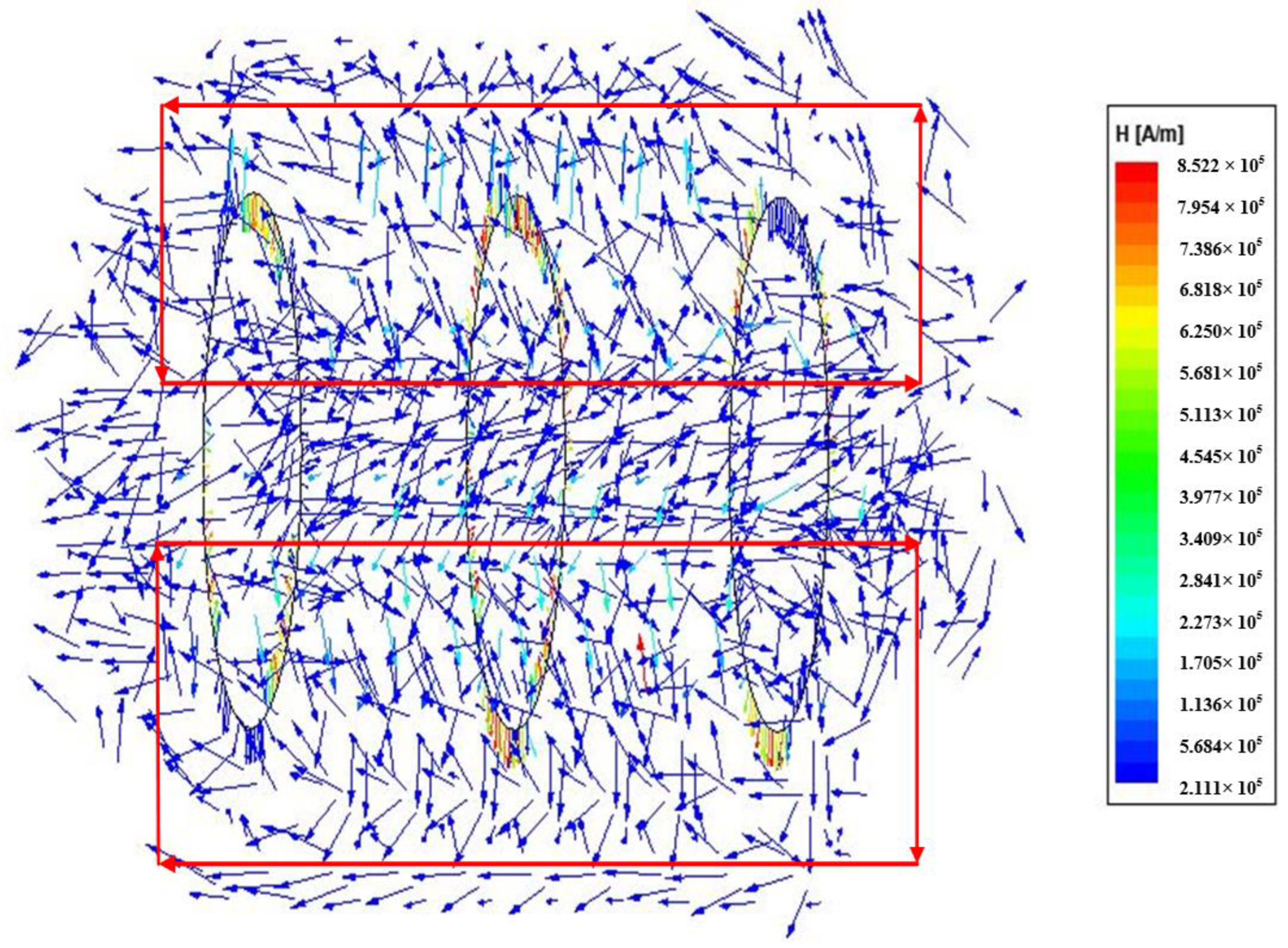
4. Simulation, Analysis and Verification

The actual motor model parameters are shown in the following table,

Table 1. Main parameters of the hybrid excitation motor.

Parameter	Numeric Value	Parameter	Numeric Value
Stator core outer diameter Dso/mm	234	Rotor core outer diameter Dro/mm	154
Stator core inner diameter Dsi/mm	160	Rotor core inner diameter Dri/mm	20
Number of stator slots Q	72	Permanent magnet thickness hpm/mm	14
Axial length of the alternating polar part ljc/mm	30	Gas length hg/mm	2
Axial length of the permanent magnet part lpm/mm	135	Pole embrace	0.85
Number of pole-pairs	3	Remanent flux density	1.23

.

Using Ansys Maxwell Electromagnetics Suite 2022 R1 software, a simulation model was established to obtain a magnetic vector map for the above motor, as shown in Figure 5. When the annular exciting winding passes the 7.5 A current, the trend of the magnetic field intensity in the motor is shown by the red line in Figure 5, which indicates that the magnetic circuit of the motor is divided into radial and axial directions, and the magnetic flux can be adjusted by adjusting the exciting current.

From Figure 5, it can be seen that the vector magnetic field flows along the axial path as shown by the red line in Figure 5; at the end, due to the staggered distribution of magnetic poles at both ends and a certain angle of misalignment, the direction of magnetic field strength distribution at both ends is asymmetric; however, it has a specific pattern.

From Figure 6, it can be seen that, when the excitation current is not applied to the ring excitation winding, the air-gap flux density distribution in the full permanent magnet part of the motor is uniform, the air-gap magnetic density distribution in the staggered magnetic pole part is essentially symmetrical, and the magnetic field strength in the ferromagnetic pole part is relatively low. It can be seen that using Maxwell software can better display the three-dimensional magnetic field distribution of the motor.

When the current of the ring excitation winding is 0, the induced electromotive force waveform is as shown in Figure 7, which can meet the output requirements of the motor’s no-load voltage. The radial and tangential magnetic compact waveforms of the full permanent magnet part of the motor are shown in Figure 8 and Figure 9.

As shown in Figure 10, the maximum error between the analytical method and the two-dimensional finite element method is 0.94%, which meets actual engineering requirements. We conducted the magnetic field analysis of the motor in this case at the same workstation, which takes 242 s to complete in the two-dimensional finite element operation, whereas the subdomain method only takes 0.961678 s to complete. It can be concluded that although the modeling process of the subdomain method is complex, the analysis time will be greatly reduced during motor optimization analysis.

5. Conclusions

From the above results, the following conclusions can be drawn:

(1)

The solution results of the subdomain method are highly consistent with the finite element analysis results, indicating that the subdomain method can be used to carry out the magnetic field calculation and analysis of the motor.

(2)

In the present study, the sub-domain method was adopted considering the opening of the stator slot, and the influence of the stator slot effect could be considered. Therefore, the influence of the slot effect on motor performance can be studied to provide a basis for motor design.

(3)

Using the theory and method to solve the hybrid excitation motor equivalent to a full permanent magnet motor, the no-load magnetic field is correct and effective. This method can be used to accurately analyze and calculate the magnetic field of the hybrid excitation motor, which lays a solid foundation for further study of the motor.

References

1. Ma, W. Some thoughts on the development of frontier technology in electrical discipline. J. Electr. Technol. 2021, 36, 4627–4636. [Google Scholar]
2. Ma, W.; Lu, J. Research status and challenges of electromagnetic emission technology. J. Electr. Technol. 2023, 38, 3943–3959. [Google Scholar]
3. Ma, W. The direction of ship power development-Integrated power system. J. Nav. Univ. Eng. 2002, 14, 1–5. [Google Scholar]
4. Fu, L.; Liu, L.; Wang, G.; Ma, F.; Ye, Z.; Ji, F.; Liu, L. Research progress of MV DC integrated power system in China. China Ship Res. 2016, 11, 72–79. [Google Scholar]
5. Di Barba, P.; Bonislawski, M.; Palka, R.; Paplicki, P.; Wardach, M. Design of Hybrid Excited Synchronous Machine for Electrical Vehicles. IEEE Trans. Magn. 2015, 51, 2424392. [Google Scholar] [CrossRef]
6. Mörée, G.; Leijon, M. Overview of Hybrid Excitation in Electrical Machines. Energies 2022, 15, 7254. [Google Scholar] [CrossRef]
7. Zhao, J.; Lin, M.; Fu, X.; Huang, Y.; Xu, D. An Overview and New Progress of Hybrid Excited Synchronous Machines and Control Technologies. Proc. Chin. Soc. Electr. Eng. 2014, 34, 5876–5887. [Google Scholar]
8. Di Barba, P.; Mognaschi, M.E.; Bonislawski, M.; Palka, R.; Paplicki, P.; Piotuch, R.; Wardach, M. Hybrid excited synchronous machine with flux control possibility. Int. J. Appl. Electromagn. Mech. 2016, 52, 1615–1622. [Google Scholar] [CrossRef]
9. Cinti, L.; Michieletto, D.; Bianchi, N.; Bertoluzzo, M. Hybrid Excited Permanent Magnet Motor: Analytical Sizing, Finite Element Analysis and Tests. IEEE Trans. Ind. Appl. 2023, 59, 6645–6654. [Google Scholar] [CrossRef]
10. Lin, N.; Wang, D.; Wei, K.; Cheng, S.; Yi, X. Structure and voltage regulating performance of high-speed mixed excitation generator. J. Electrotech. Technol. 2016, 31, 19–25. [Google Scholar]
11. Liu, F.; Wang, X.; Xing, Z.; Yu, A.; Li, C. Reduction of cogging torque and electromagnetic vibration based on different combination of pole arc coefficient for interior permanent magnet synchronous machine. CES Trans. Electr. Mach. Syst. 2021, 5, 291–300. [Google Scholar] [CrossRef]
12. Zhu, Z.; Howe, D. Instantaneous magnetic field distribution in brushless permanent magnet DC motors. Part I: Open-circuit field. IEEE Trans. Magn. 1993, 29, 124–135. [Google Scholar] [CrossRef]
13. Faradonbeh, V.Z.; Rahideh, A.; Boroujeni, S.T.; Markadeh, G.A. 2-D. Analytical No-Load Electromagnetic Model for Slotted Interior Permanent Magnet Synchronous Machines. IEEE Trans. Energy Convers. 2021, 36, 3118–3126. [Google Scholar] [CrossRef]
14. Faradonbeh, V.Z.; Rahideh, A. 2-D analytical on-load electromagnetic model for double-layer slotted interior permanent magnet synchronous machines. IET Electr. Power Appl. 2022, 16, 394–406. [Google Scholar] [CrossRef]
15. Teymoori, S.; Rahideh, A.; Moayed-Jahromi, H.; Mardaneh, M. 2-D Analytical Magnetic Field Prediction for Consequent-Pole Permanent Magnet Synchronous Machines. IEEE Trans. Magn. 2016, 52, 1–14. [Google Scholar] [CrossRef]
16. Ruda, A.; Louf, F.; Boucard, P.-A.; Mininger, X.; Verbeke, T. A parallel implementation of a mixed multiscale domain decomposition method applied to the magnetostatic simulation of 2D electrical machines. Finite Elements Anal. Des. 2024, 235, 104136. [Google Scholar] [CrossRef]
17. Tapia, A.; Leonardi, F.; Lipo, T.A. Consequent-pole permanent-magnet machine with extended field-weakening capability. IEEE Trans. Ind. Appl. 2003, 39, 1704–1709. [Google Scholar] [CrossRef]
18. Wang, D. Mathematical model and equivalent analysis of new hybrid excitation synchronous motor. J. Electr. Technol. 2017, 32, 149–156. [Google Scholar]
19. Cao, G.; Ye, C.; Deng, C.; Wan, S.; Liu, K.; Yao, K.; Qi, X.; Lu, J.; Wang, Z. Theoretical Analysis for Rapid Design of Hybrid Excitation Synchronous Machine with Consequent Pole Rotor. IEEE Trans. Transp. Electrif. 2024, 1-1. [Google Scholar] [CrossRef]
20. Wu, L.; Yin, H.; Wang, D.; Fang, Y. A Nonlinear Subdomain and Magnetic Circuit Hybrid Model for Open-Circuit Field Prediction in Surface-Mounted PM Machines. IEEE Trans. Energy Convers. 2019, 34, 1485–1495. [Google Scholar] [CrossRef]
21. Wang, Q. Practical Design of Magnetostatic Structure Using Numerical Simulation; Wiley & Sons: Hoboken, NJ, USA, 2013. [Google Scholar]
22. Pang, L.; Zhao, C.; Shen, H. Research on Tangential Magnetization Parallel Magnetic Path HybridExcitation Synchronous Machine. J. Electr. Eng. Technol. 2022, 17, 2761–2770. [Google Scholar] [CrossRef]
23. Wang, H.; Guan, P.; Liu, S.; Wu, S.; Shi, T.; Guo, L. Modeling and Analyzing for Magnetic Field of Segmented Surface-Mounted PM Motors with Skewed Poles. J. Electr. Eng. Technol. 2022, 17, 1097–1109. [Google Scholar] [CrossRef]
24. Ma, J.; Gu, F.; Wang, L.; Ma, S.; Golmohammadi, A.-M.; Zhang, S. The Design and Optimization of a Novel Hybrid Excitation Generator for Vehicles. World Electr. Veh. J. 2024, 15, 139. [Google Scholar] [CrossRef]
25. Pang, L.; Zhao, C.; Shen, H. Properties of Adjust Magnetic Field of Hybrid Excitation Synchronous Machine with Tangential Accumulation of Magnetic Field Shunt-wound Magnetic Path. In Proceedings of the 2021 24th International Conference on Electrical Machines and Systems (ICEMS), Gyeongju, Republic of Korea, 31 October–3 November 2021; pp. 1538–1543. [Google Scholar]
26. An, Y.; Ma, C.; Zhang, N.; Guo, Y.; Degano, M.; Gerada, C.; Bu, F.; Yin, X.; Li, Q.; Zhou, S. Calculation Model of Armature Reaction Magnetic Field of Interior Permanent Magnet Synchronous Motor with Segmented Skewed Poles. IEEE Trans. Energy Convers. 2022, 37, 1115–1123. [Google Scholar] [CrossRef]
27. Zhang, W.; Pang, L.; Hu, H.; Qin, H.; Zhao, C. The effect of excitation current on radial electromagnetic force wave of tangential magnetizing parallel structure hybrid excitation synchronous motor. Int. J. Appl. Electromagn. Mech. 2024, 74, 209–233. [Google Scholar] [CrossRef]
28. Xia, C.; Guo, L.; Wang, H. Modeling and Analyzing of Magnetic Field of Segmented Halbach Array Permanent Magnet Machine Considering Gap between Segments. IEEE Trans. Magn. 2014, 50, 2336835. [Google Scholar] [CrossRef]
29. Su, W.; Guo, Y.; Wang, D.; Wei, K. Semi-Analytical Calculation of No-Load Radial and Tangential Electromagnetic Force Waves of a Non-Salient Pole Synchronous Generator. IEEE Trans. Energy Convers. 2021, 36, 2956–2966. [Google Scholar] [CrossRef]
Figure 1. Schematic diagram of the new hybrid excitation generator. (a) Two-dimensional schematic diagram of the hybrid excitation generator; (b) Two-dimensional structure diagram of the hybrid excitation generator.
Electronics 13 02574 g001
Figure 2. Cross-section diagram of the permanent magnet motor.
Electronics 13 02574 g002
Figure 3. Residual magnetization of the radial charged rotor permanent magnet.
Electronics 13 02574 g003
Figure 4. Residual magnetization of the permanent magnet of the radial charged rotor.
Electronics 13 02574 g004
Figure 5. Space magnetic vector diagram of the hybrid excitation motor.
Electronics 13 02574 g005
Figure 6. Air-gap flux density distribution of the hybrid excitation motor. (a) Full permanent magnet partial air-gap magnetic density; (b) Alternating polar partial air-gap magnetic density.
Electronics 13 02574 g006
Figure 7. Waveform diagram of the output voltage of the hybrid excitation motor.
Electronics 13 02574 g007
Figure 8. Radial air-gap flux density distribution (analytical method).
Electronics 13 02574 g008
Figure 9. Tangent air-gap flux density distribution (analytical method).
Electronics 13 02574 g009
Figure 10. Radial air-gap magnetic dense waveform (comparison between the analytical method and finite element method).
Electronics 13 02574 g010