Detection and Classification of Obstructive Sleep Apnea Using Audio Spectrogram Analysis

Abstract

Sleep disorders are steadily increasing in the population and can significantly affect daily life. Low-cost and noninvasive systems that can assist the diagnostic process will become increasingly widespread in the coming years. This work aims to investigate and compare the performance of machine learning-based classifiers for the identification of obstructive sleep apnea–hypopnea (OSAH) events, including apnea/non-apnea status classification, apnea–hypopnea index (AHI) prediction, and AHI severity classification. The dataset considered contains recordings from 192 patients. It is derived from a recently released dataset which contains, amongst others, audio signals recorded with an ambient microphone placed ∼1 m above the studied subjects and apnea/hypopnea accurate events annotations performed by specialized medical doctors. We employ mel spectrogram images extracted from the environmental audio signals as input of a machine-learning-based classifier for apnea/hypopnea events classification. The proposed approach involves a stacked model which utilizes a combination of a pretrained VGG-like audio classification (VGGish) network and a bidirectional long short-term memory (bi-LSTM) network. Performance analysis was conducted using a 5-fold cross-validation approach, leaving out patients used for training and validation of the models in the testing step. Comparative evaluations with recently presented methods from the literature demonstrate the advantages of the proposed approach. The proposed architecture can be considered a useful tool for supporting OSAHS diagnoses by means of low-cost devices such as smartphones.

1. Introduction

Sleep, which accounts for a third of human life, is of great importance for maintaining health [1]. Unfortunately, a hidden sleep disorder known as obstructive sleep apnea–hypopnea syndrome (OSAHS) negatively affects the quality of life for many individuals [2,3].

OSAHS is primarily caused by the constriction of the upper airways at different levels. While increased muscle tone during wakefulness prevents the collapse of the upper airways, during sleep, a combination of extraluminal pressure from surrounding soft tissues and negative intraluminal pressure during inspiration can lead to upper airway collapse. In addition, obese people may experience further narrowing of the upper airways, which leads to even more pronounced clinical consequences. In individuals affected by sleep apnea, sleep quality may deteriorate, leading to daytime sleepiness, memory impairment, increased risk of accidents due to excessive sleepiness, and overall decreased productivity. In more severe cases, adults with OSAHS can develop conditions such as high blood pressure, coronary heart disease, stroke, cardiac arrhythmias, and other related conditions. Additionally, in infants, OSAHS can also lead to behavioral disorders and, in extreme cases, even sudden death [4]. People affected by this condition, especially adults, have an increased risk of causing traffic accidents. Moreover, they often suffer from mood swings and depression, which contributes to the significant financial and social impact of OSAHS [5]. Nowadays, approximately 6–13% of the world population suffers from this disease [6], but 80% of apnea patients remain undiagnosed [7]. To represent the severity of OSAHS, a specific parameter called “apnea/hypopnea index” (AHI) is used. This index counts the number of apneas and hypopneas per hour of sleep. A single apnea event occurs when peak inspiratory flow falls below 10% of baseline for at least 10 s [8]. OSAHS is classified as mild if the AHI is in the [5–15] range, moderate if the AHI is in the [16–30] range and severe if the AHI is above 30. To determine the AHI, patients must undergo a clinical examination known as polysomnography (PSG), which is usually performed in a hospital. During PSG, various biosignals are recorded, including breathing patterns, heart rate, movements, snoring, oxygen saturation, pharyngeal movements, and others. To capture all these signals, patients must wear sensors that can simultaneously capture and convert them into electrical signals. A recording device then acquires these electrical signals via cables. The presence of these cables, sensors, and devices can cause discomfort for patients, particularly in a setting that differs from the comfort of their own bedroom [9]. As a result, OSAHS diagnoses often go unrecognized, resulting in a significant number of individuals affected by OSAHS remaining untreated [10]. Therefore, it is crucial to promote the advancement of equipment and technologies that can facilitate the diagnosis of OSAHS in a more comfortable way [11].

The aim of the present study is along these lines. Indeed, we investigate the ability to recognize OSAHS just by recording an audio signal, which is subsequently processed with machine learning (ML) approaches to determine the AHI. The proposed investigation starts with an analysis of the audio signal in the frequency domain to obtain mel spectrograms. A spectrogram is a visual representation of the spectrum of frequencies in a signal changing over time. It is a three-dimensional graph where the x-axis represents time, the y-axis represents frequency, and the color intensity or darkness represents the strength of the signal’s energy at each time and frequency. A mel spectrogram is a type of spectrogram that takes into account the principles of human auditory perception, known as psychoacoustic [12]. It is derived from a standard spectrogram but uses a mel scale to map the frequency content of the signal to a perceptually relevant scale. The mel scale is a nonlinear scale that mimics the sensitivity of the human ear to different frequencies. In a mel spectrogram, the frequency axis is divided into mel frequency bins and the intensity of each bin is represented by a color or gray scale, similar to a conventional spectrogram.

VGGish networks, designed for audio classification tasks [13], take these mel spectrograms as input representations and extract high-level features that contribute to the network’s ability to recognize and categorize audio signals.

Since the main objective of this work is the identification/classification of obstructive sleep apnea–hypopnea syndrome events based on features extracted from audio signals recorded during sleep, we investigated the capability of VGGish-based architectures widely used for audio classification. Specifically, we developed a bidirectional network with long short-term memory (bi-LSTM) trained to classify input sequences obtained from a pretrained VGGish network using a transfer learning (TL) approach.

This latter architecture was already presented in [14], where preliminary results were investigated using a reduced subgroup of patients. Specifically, in [14], we proposed a pretrained network based on a VGGish model to perform “apnea” detection based on audio signal processing. The network was trained to classify mel spectrograms extracted from audio signals with a duration of 1 s according to an “apnea”/“no-apnea” classification. To determine the output class for excerpts with a duration of 5 to 15 s, each individual prediction obtained with a step of 250 ms was combined with a majority decision rule. The analysis was performed on audio excerpts from a subset of 25 patients from the dataset described in [15]. We extracted 860 clips that were evenly distributed across both classes. We analyzed confusion matrix charts and compared the performance of our approach with the support vector machine-based classifiers proposed in [16], which served as a baseline.

The present study represents a significant advance by extending and building on these results:

• Increasing the subgroup of patients from 25 to 192;
• Performing the training and testing of the networks using a separate subset of data related to the patients (i.e., no data from patients used in the training appears in the test);
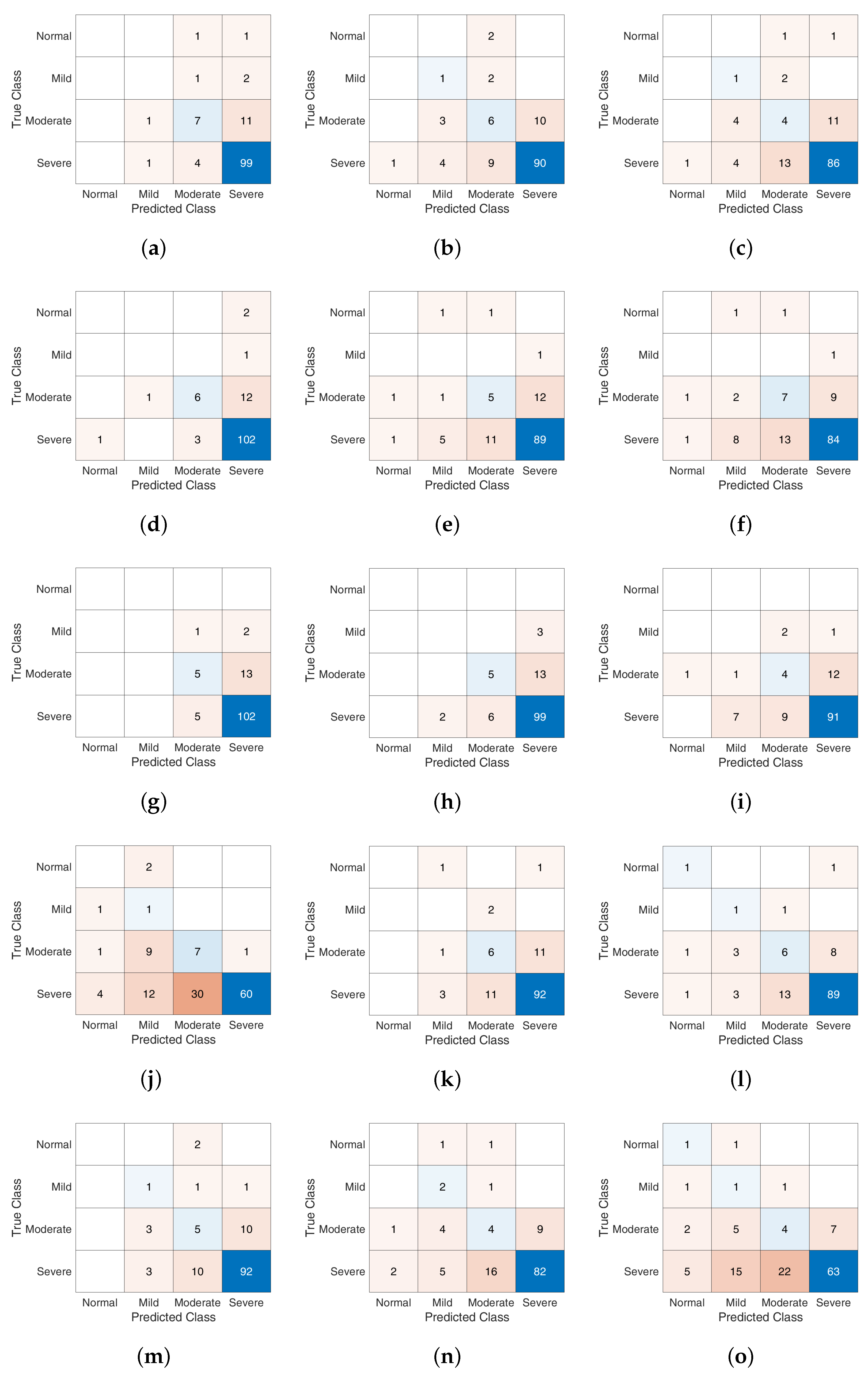
• Presenting the bi-LSTM architecture and performance comparisons in terms of confusion matrix for the identification of OSAHS;
• Providing results related to AHI prediction and AHI severity classification.

The remaining of the paper is organized as follows: Section 2 presents related work; in Section 3, the used dataset is described; the proposed methodology for the classification of apnea events is described in Section 4, the analysis of the simulation results is provided in Section 5; finally, the conclusions are drawn in Section 6.

2. Related Works

Recently, several researchers have focused on the sound-based identification of OSAHS. In an early attempt to tackle this problem, researchers presented a snoring sound classifier using CNNs for spectrogram image analysis, as described in [17]. Amiriparian et al. used the Munich–Passau Snore Sound Corpus as their dataset, which includes 828 snoring samples categorized into four classes representing the location of the obstruction leading to snoring: velum, oropharynx, tongue, and epiglottis. Despite the potential of snoring as an indicator of obstructive sleep apnea and hypopnea syndrome (OSAHS), it is worth noting that the dataset did not include annotations on the occurrence of apnea episodes. In [16], the authors proposed a system for identifying OSAHS based on video and audio recordings of a patient. The audio analysis involved the extraction of three different features: a mixed collection of acoustic and prosodic parameters, features derived from applying wavelet packet transform (WPT) to the spectrogram of the signal, and features obtained through the application of non-negative matrix factorization (NMF) to the spectrogram. The entire audio signal, recorded at a rate of 16 kHz with 16 bits per sample for each patient, was divided into 10 s intervals, with a 5 s overlap between consecutive segments. Each audio segment was further subdivided into subsegments, each spanning a time length of 5 s with a step interval of 0.5 s. The spectrogram for each subsegment was generated using a short-time Fourier transform (STFT) with an STFT window of 25 ms and step sizes of 12.5 ms. For the experimental setup and performance evaluation, the authors used a proprietary dataset with recordings of four patients over two different nights, with each recording session lasting approximately 480 min. The video and audio recordings were synchronized with the polysomnography (PSG) signals and then manually classified into four different classes: (i) central apnea, (ii) obstructive or mixed apnea, (iii) hypopnea, and (iv) all other events indicated in the ground truth labels. The authors used both support vector machines (SVMs) and neural networks (NNs) as classifiers. Considering only the audio component, the highest accuracy (99.17%) was obtained with an SVM classifier using features extracted through non-negative matrix factorization (NMF). To obtain the above results, an inverse 5-fold cross-validation (CV) was used (1-fold for training and the remaining 4-fold for testing).

An algorithm for OSAHS detection based on convolutional neural networks (CNNs) was presented in [18]. The authors used mel frequency cepstral coefficients (MFCCs) as audio features extracted with a 40 ms time window. Three CNN architectures, namely, VGGNet [19], Inception (GoogLeNet) [20], and ResNet [21], were evaluated. The performance of the algorithm, measured by accuracy on the same dataset as in [17], was compared with a baseline algorithm using a Gaussian mixture model (GMM) as a classifier. Both the proposed CNN architectures and the baseline algorithm exhibited remarkably poor OSAHS classification performance, consistently falling below 50%. Moreover, the annotation methodology for apnea events in the snoring-based dataset of [17] remains unclear.

The authors of [22,23] presented a wearable system that uses audio sensors to recognize various human contexts, including breathing, heartbeat and swallowing. The device has two different microphones—an open-air microphone and a contact microphone—which are both integrated into the same body and record audio signals simultaneously. To determine the optimal placement of the device and to evaluate the classification accuracy for five different audio events (breathing, swallowing, movement, oral sounds, and others), a special dataset was created. This dataset includes recordings of seven healthy individuals simulating typical movements and sounds associated with a sleeping person. From the audio signal sampled at 44,100 Hz, a feature vector with 28 MFCCs and another vector with 14 parameters derived from 10 fast Fourier transform (FFT) peaks and 4 statistical and temporal features extracted from windows of 1, 2, and 3 s with a step of 0.25 s were obtained. These vectors were used to train models based on SVM and random forest (RF). A time frame of 4 min within the total recording time of 5 min for each actor was used for training, while the remaining 1 min was used for testing. The study presented performance results and comparisons using data from individual microphones as well as aggregated data. Although the potential of the proposed wearable device and optimal positioning on the patient’s body to improve recording quality was emphasized, the classification results were based on a small simulated dataset and lacked appropriate OSAHS annotations, which are two major limitations in demonstrating the effectiveness of this approach for OSAHS classification.

A commonly used approach to identify OSAHS is to classify the snoring sounds. In [24], the authors proposed an automatic detection method to identify snoring segments from sleep sounds using acoustic feature analysis and an SVM algorithm. The authors of [25] collected sleep sounds from 32 volunteers (including 16 normal people and 16 OSAHS patients) for a whole night (8 h) via a microphone at a sampling frequency of 16 kHz. Then, they extracted snoring sounds of 3 s duration using a speech endpoint detector [26]. According to the PSG, the snoring data were divided into two categories: the positive sample (normal snoring), which included the data of nocturnal snoring of normal people, and the negative sample (abnormal snoring), which included the data of nocturnal snoring of OSAHS patients recorded in the middle and at the end of the apnea event. Three feature extraction methods (MFCC, LPCC, LPMFCC) and three neural-network-based models (3-layer CNN, 5-layer CNN, and LSTM) were combined to evaluate the performance in terms of accuracy, sensitivity, specificity, precision, and F1-score. The results showed that the MFCC-LSTM combination performed best, with the accuracy of classification reaching 0.87. The previous approach was improved in [27] thanks to the additional use of three other audio features with different functions, used to describe the temporal–spatial pattern of the snoring data, as input of the LSTM. With a dataset of 30 patients, an accuracy of 95.3% was achieved. It is important to note that this accuracy refers to the classification of normal/abnormal snoring and not to the detection of apneas. Based on the detection of abnormal snorers in a night and counting them, it is possible to estimate the AHI. In any case, the results are influenced by the correctness of the automatic detection of the endpoints of snoring sounds.

Recently, in 2023, a model was proposed to study the distribution characteristics of snoring sounds during the night to distinguish simple snorers and OSAHS patients [28]. Based on a large number of features, including MFCC, perceptual linear predictive (PLP), Bark sub-band feature (BSF), spectral entropy (SE), 800 Hz power ratio (PR800), pitch frequency (F0), formants (F1, F2, and F3), and gammatone cepstral coefficient (GTCC), the authors applied a Fisher-ratio-based feature selection method. The GMM was proposed to investigate the acoustic characteristics of snoring sounds throughout the night and to classify simple snorers or OSAHS patients. To validate the proposed model, a cross-validation experiment was conducted based on 30 subjects (leave-one-subject-out). The proposed model achieved an average accuracy of 90.0% and an average precision of 95.7% using selected features. In the same year, the authors of the latter paper proposed another relevant work [29], in which they estimated the AHI by analyzing snoring sounds. Three primary models were used to investigate the discrimination between abnormal and normal snoring sounds: acoustic features combined with XGBoost, mel spectrum coupled with CN, and mel spectrum integrated with the residual neural network. A fusion model strategy using soft voting was then implemented to merge these three models and create a model characterized by high robustness and effectiveness. The identified abnormal snoring sounds were used to form apnea–hypopnea events, and the AHI was then calculated based on the number of these events and the recording duration. In this study, a total of 40 subjects from the First Affiliated Hospital of Guangzhou Medical University and Korompili’s were used. A pretrained VGG19 and LSTM model was proposed to classify the snoring sounds of simple snorers and OSAHS patients and to detect apnea–hypopnea snoring from the whole night recorded sounds of patients in [30]. The proposed model achieved an accuracy of 99.31% in classifying simple snorers’ snoring and OSAHS patients, while an accuracy of 85.21% and 66.29% was achieved for discriminating normal snoring and apnea–hypopnea snoring from patients based on hold-out and leave-one-subject-out validation methods, respectively. The sounds of 50 subjects were recorded throughout the night and subsequently validated by the work of Wang et al. [24] and segmented to obtain relatively clean snoring sounds.

A limitation of this work based on the classification of snoring sounds arises from the need to segment the audio signal in order to define the boundaries of the signal containing the snoring. The reported accuracy performances are based on the assumption that the automatic segmentation system does not make errors in the identification of snoring sounds. Even though the number of subjects is still too small for statistical purposes, these promising results demonstrate that the diagnosis of OSAHS patients is possible using sound recordings at home.

In 2021, a publicly available dataset of 212 polysomnograms accompanied by synchronized high-quality tracheal and ambient microphone recordings was provided in [15]. The entire dataset was manually annotated by medical experts and categorized into different apnea events such as “Obstructive Apnea”, “Central Apnea”, “Mixed Apnea” and “Hypopnea”. Consequently, we believe that this dataset is an important milestone for evaluating and comparing the performance of classifiers for obstructive sleep apnea and hypopnea syndrome (OSAHS), especially those based on audio signal recordings.

In this work, we used this large dataset to propose an OSAHS classification approach based on CNNs that can be considered statistically significant. Specifically, we used a pr-trained network based on a VGGish model, which is commonly used in sound classification. We propose a classification system based on a continuous detection of the audio signal without any segmentation of the snoring sounds. We evaluate the performance of our proposed “bi-LSTM combined with VGGish” architecture and discuss the results in comparison with recent research on OSAHS and AHI classification [28,29,30]. Performances are evaluated using a 5-fold cross-validation (1-fold for training and 4-fold for testing), excluding, during the testing phase, sounds recorded by subjects used in the training phase.

3. OSAHS Dataset

As described in the publication by Korompili et al. (2021) [15], data were collected from a cohort of 212 subjects seeking a diagnosis of sleep apnea syndrome (SAS) at the Sleep Study Unit of the Sismanoglio—Amalia Fleming General Hospital in Athens. The audio signals were recorded with a portable two-channel multitrack recorder (Tascam DR-680 MK II, TEAC AMERICA, INC., Santa Fe Springs, CA, USA) and synchronized with the PSG data. The first channel was connected to a contact microphone (Clockaudio CTH100, Clockaudio Ltd., Waterlooville, Hampshire, UK) placed on the patient’s trachea. Simultaneously, the second channel was connected to an ultra-linear measurement condenser microphone (Behringer ECM8000, Behringer, Willich, Germany) positioned approximately 1 m above the patient’s bed, specifically over the head area. Both sound signals were sampled at a rate of 48 kHz and originally recorded at 24 bits per sample. To facilitate storage in European Data Format (EDF) while maintaining synchronization with other polysomnography signals, the bit depth per sample was later reduced to 16. The PSG data comprise 16 channels, incorporating electroencephalogram (EEG), electroculogram (EOG), leg movement signal, electrocardiogram (ECG), RR interval in the ECG, pulse rate derived from the ECG, changes in thoracic volume, changes in abdominal volume, the nasal/oral flow pressure, the body position, and the oxygen content of the blood (oxygen saturation). The PSG study is conducted by medical professionals in the Sleep Studies Department of the Sismanoglio–Amalia Fleming General Hospital in Athens. Each patient’s recordings are analyzed by two specialists according to “sleep stages” and “apnea events” scoring. First, a certified technician performs the initial evaluation stage, followed by a final evaluation performed by a highly experienced and certified doctor with 30 years of experience. In this final assessment, the actual positively annotated events are reviewed and any missed events are added to ensure a comprehensive assessment. The original dataset includes EDF files containing polysomnogram signals for 287 patients, along with RML files containing all annotations provided by the medical team of the Sismanoglio General Hospital of Athens. For our study, we only considered the annotations of the medical team after the automatic rejection of the false-positive apneas, whose annotations appear in the subfolder named “APNEA_RML_clean”. The folder contains annotations for 194 patients. For each patient, we downloaded the rml file with the annotations and the corresponding edf file from the folder “APNEA_EDF” with the PSG signals and audio recordings. From this latter, we extracted the channel number 20, containing the ambient microphone (placed 1 m above patient head) recordings. We had to remove the recordings of 2 patients (id “00001339” and “00001394”) due to errors in the management of the associated edf files. We then downsampled each recording to 16,000 samples per second using “sox” [31] and saved all files in Microsoft RIFF wav format. In our experiments, we only used the audio signals recorded from the ambient microphone. Microphones are characterized by several features: polar pattern, impedance, sensitivity, frequency response, and dynamic range.

The microphone used to record the ambient audio signals on channel 20 of the dataset is a Behringer ECM8000. It has an omnidirectional characteristic, i.e., it picks up sound evenly from all directions and is therefore ideal for recording ambient sounds. It has an impedance of 200 ohms, which ensures compatibility with most audio equipment and helps reduce signal loss. The sensitivity is −39.2 dBV/Pa, which means that even quiet sounds can be picked up clearly and distinctly. The frequency response of 20 Hz to 20,000 Hz enables precise reproduction of the entire spectrum of human hearing and ensures high-fidelity sound recording.

In our vision of a possible application of the proposed OSAHS automatic recognition system, based on the processing of audio signals, we took into account the very high prevalence of smartphones in people’s everyday lives. For their original function as a phone, these devices are all equipped with microphones. Usually, people do not switch off their device at night if they have it lying on their bedside table. Accordingly, for future applications, smartphones can be considered good candidates for capturing audio signals during the night, which can then be processed for automatic OSAHS diagnosis.

Nowadays, smartphones are equipped with high-quality microphones that have evolved considerably in recent years. Modern smartphone microphones use technology based on micro-electromechanical systems (MEMSs), as they are very small, robust, and powerful. They can have both omnidirectional and directional polar patterns. Many smartphones use multiple omnidirectional and directional microphones to improve sound recording quality and enable noise reduction features. To ensure compatibility with the phone’s audio processing circuits, reduce signal loss, capture a broad spectrum, and ensure high-quality audio recording suitable for both speech and ambient sounds, smartphone microphones typically have low impedance (∼200 ohms), high sensitivity (e.g., −42 dBV/Pa), and wide frequency response (20 Hz to 20,000 Hz). In addition, multiple microphones are typically used to filter out background noise for clearer voice pickup in noisy environments. The characteristics of the MEMS microphones in today’s smartphones seem to be similar to or better than those of the Behringer ECM8000. Accordingly, we can assume that the results obtained with this dataset can be easily transferred to real-world applications to achieve analogue performance.

The annotations of type “Respiratory” were used as a reference and, in particular, grouped into two classes. The first, named “Apnea”, includes the events “Central Apnea”, “Hypopnea”, “Mixed Apnea”, “Obstructive Apnea” and “Periodic Breathing”. The second, called “No-Apnea”, includes everything that does not belong to the “Apnea” class. To extract data from the two classes in a balanced way, we processed the recordings for each patient and the corresponding annotation file. To obtain apnea/non-apnea excerpts, we analyzed each audio segment whose samples fell into the corresponding category and extracted sequences with a duration of 5 s with a step of 10 s. We divided each segment into evenly spaced windows of 5 s. the files of the “Apnea” segments were labeled with the “patient number”, the label “IN”, a label referring to the apnea category, such as “CA” = “Central Apnea”, “HA” = “Hypopnea”, “MA” = “Mixed Apnea”, “OA” = “Obstructive Apnea”, “PR” = “Periodic Respiration”, and a sequential number for each patient and subcategory. The “No-Apnea” extracts were named with the “Patient ID”, the designation “OUT”, and a consecutive number for each patient.

Table 1. Distribution of excerpts in the various classes.

Class	# Excerpts
OUT	247,542
IN	104,777
IN(CA)	3696
IN(HA)	21,819
IN(MA)	15,987
IN(OA)	63,219
IN(PR)	56

shows the number of excerpts obtained in each category.

In total, the dataset under consideration contains 352,319 nonoverlapping audio excerpts, each lasting 5 s. According to the input format required by VGGish, we extracted mel spectrograms from each audio excerpt, each representing 1 s of audio and with a step size of 0.25 s. Each spectrogram was evaluated as a matrix of 96 × 64 values: 96 is the number of 25 ms partially overlapping frames in each mel spectrogram and 64 represents the number of mel bands, ranging from 125 Hz to 7.5 kHz.

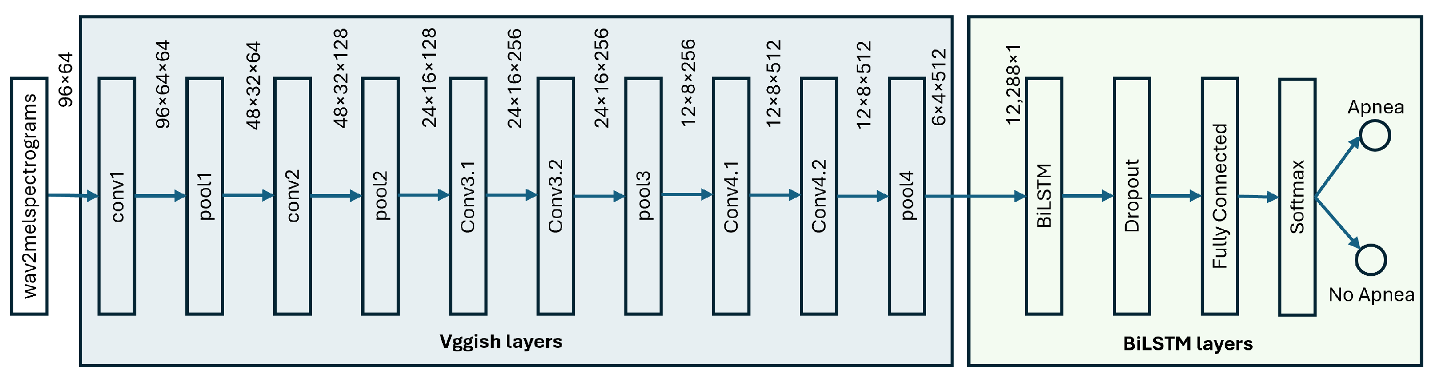
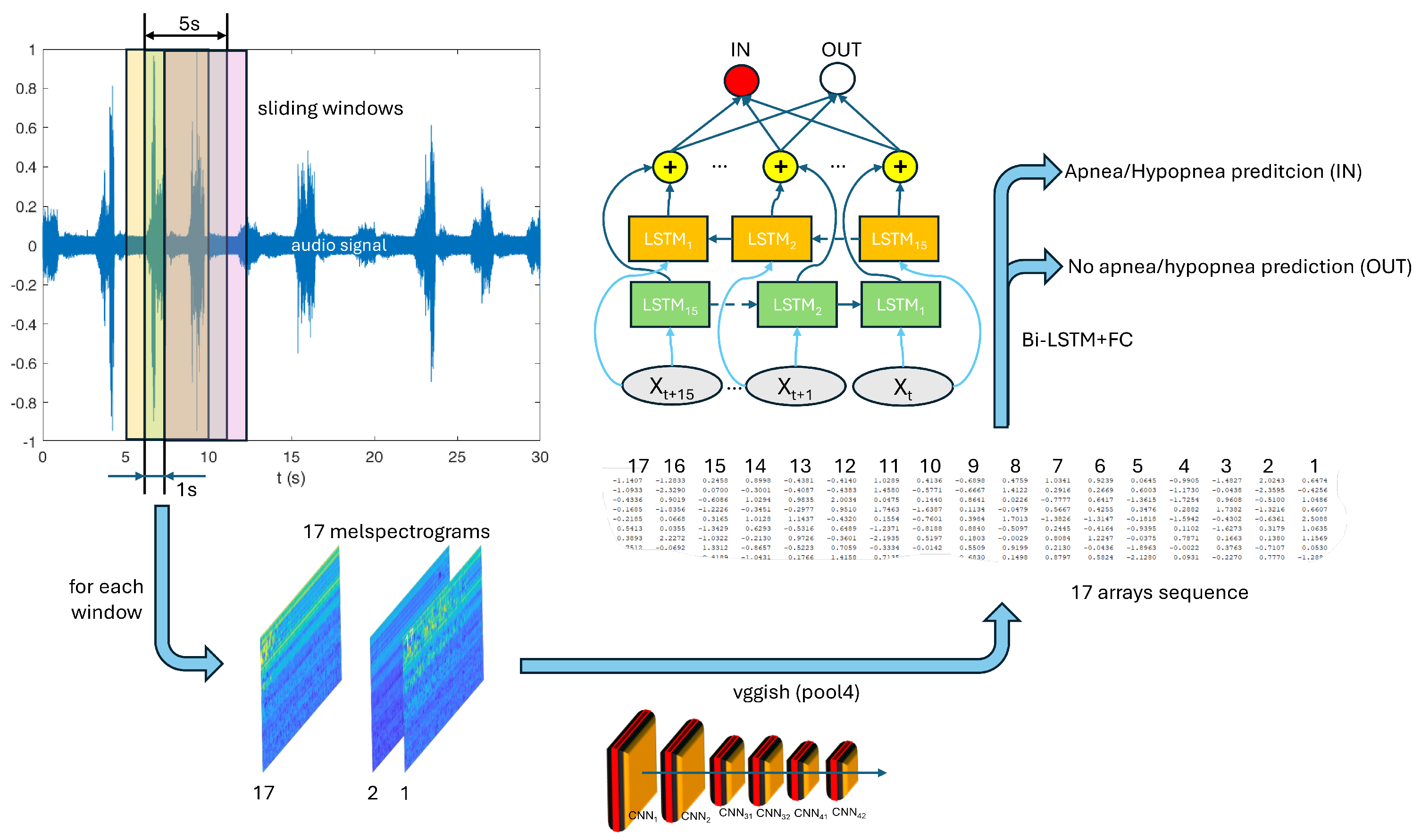
4. Proposed Methodology: Deep Neural Networks for Audio Processing

In recent years, the dramatic progress in computing power, mainly related to the introduction of massive multicore GPUs, has driven the use of deep learning techniques to develop classification and regression networks that are applied in many different fields [32]. ML approaches have been widely applied in both the fields of signal processing and telecommunication networks [33,34,35,36,37,38]. Sound classification and recognition is one of the research areas investigated, including music classification applications [39,40,41,42], speech recognition [43], and others.

In this work, among the various solutions available in the literature, we chose to use a CNN based on the VGG family, which was introduced in 2014 by the Visual Geometry Group (VGG) at the University of Oxford. CNNs are a type of artificial neural network architecture specifically designed for analyzing grid-like data, such as images or time series. They use convolutional filters to automatically extract features from the input data as they pass through multiple layers, allowing CNNs to learn increasingly complex representations of the data [44]. VGG models exemplify this approach by utilizing stacks of convolutional layers with small receptive fields (typically 3 × 3) and the rectified linear unit (ReLU) activation function to achieve state-of-the-art performance in various image recognition tasks. VGG networks have been successfully adapted for various applications, including audio classification. Building on the strengths of VGG networks, a pretrained model called VGGish was specifically designed for audio classification tasks. This model was originally adopted for image processing and subsequently adapted by Google in 2017 for use with audio signals The training was performed on a large YouTube dataset [45]. The pretrained VGGish network contains 24 layers with nine layers containing learnable weights: six convolutional and three fully connected layers. The input provided to the VGGish consists of a series of mel spectrograms obtained by decomposing the audio signals into a series of overlapped time frames. The original VGGish neural network was trained to classify a wide range (128) of sound events, including, but not limited to, various environmental sounds such as music, speech, animal calls, and mechanical noises. To build our classification model and focus on task-specific features for sleep apnea classification, we employed a piecewise TL approach. TL is an ML technique where knowledge acquired on one task is leveraged to enhance performance on a related task. In our study, we employed a bidirectional long short-term memory (bi-LSTM) network in conjunction with a pretrained VGGish model. Bi-LSTMs are particularly effective for processing sequential data, which are essential for capturing the temporal dynamics associated with sleep apnea events. The bidirectional nature of bi-LSTMs allows them to analyze sequences in both forward and backward directions, enhancing their ability to understand context and dependencies within the data. This approach leverages the strengths of bi-LSTMs in temporal modeling to accurately classify and identify patterns indicative of obstructive sleep apnea. Accordingly, we built a neural network architecture consisting of two submodels:

• The first submodel consists of the VGGish convolutional stages up to the “pool4” layer; this submodel is not trained further and it works with the same hyperparameters of the original VGGish;
• On the top of the previous submodel, a bi-LSTM network runs: it uses as input the output of the VGGish at the “pool4” layer and it is specifically trained to classify “Apnea” and “No-Apnea” events.

Figure 1 shows examples of sequences of mel spectrograms for “Apnea” categories and in “No-Apnea” state. It highlights difference between the “Apnea” and “No-Apnea” state. All the “Apnea” categories of the patient show continuous energy distribution on the middle- and low-frequency bands. It is evident that there is a noncontinuous distribution of energy in a specific band for sound captured in “No-Apnea” state. Moreover, the sequences of spectrograms extracted in “Apnea” state show an almost stationary behavior over the time, while spectrograms extracted in “No-Apnea” state are most irregular. This last behavior can be captured by a bi-LSTM network, and it justifies its use in our architecture.

The block scheme of the proposed architecture is depicted in Figure 2; the sizes written at the output of each layer are related to the processing of a single mel spectrogram, showcasing the flow of information from the input through the VGGish and bi-LSTM layers to the final classification output.

We constructed our model using MATLAB Version 23.2.0.2515942 (R2023b) Update 7 [46] and we ran training/validation and test on a Dell Server model PowerEdge R740xd, equipped with 2 × Intel(R) Xeon(R) Gold 6238R CPU @ 2.20 GHz, 6 × 64 GB RAM modules, 4 × GPU TESLA M10 with 8 GB memory.

To obtain input sequences for training the bi-LSTM network, we process each wav file of the dataset, which lasts 5 s, to extract the corresponding sequence of mel spectrograms (96 × 64 × 17). These sequences are the input to the VGGish network and are processed to obtain the activations at the output of layer “pool4” (12,288 × 17). These last 17 vectors with 12,288 elements are the input for the bi-LSTM network. By processing all 352,319 audio excerpts of the dataset, we obtained so many sequences that form the dataset used for defining the architecture, setting the thresholds, training, and testing the bi-LSTM network. We divided this dataset into 6 distinct folds, with each fold containing the sequences extracted from the audio excerpts of 32 patients. Consequently, sequences from each patient are exclusively present in one of the 6 folds. Patients were randomly assigned to each fold, and

Table 2. Association of patient IDs with folds.

	Fold #1 (${\mathcal{R}}_1$)	Fold #2 (${\mathcal{R}}_2$)	Fold #3 (${\mathcal{R}}_3$)	Fold #4 (${\mathcal{R}}_4$)	Fold #5 (${\mathcal{R}}_5$)	Fold #6 (${\mathcal{R}}_6$)
#1	00001000	00001014	00001028	00001008	00000995	00000999
#2	00001010	00001022	00001041	00001016	00001037	00001006
#3	00001039	00001093	00001088	00001059	00001045	00001018
#4	00001069	00001104	00001116	00001082	00001084	00001020
#5	00001097	00001131	00001122	00001089	00001086	00001024
#6	00001106	00001147	00001126	00001139	00001095	00001026
#7	00001108	00001155	00001135	00001151	00001110	00001043
#8	00001120	00001172	00001137	00001153	00001112	00001057
#9	00001157	00001176	00001169	00001161	00001127	00001071
#10	00001195	00001197	00001210	00001171	00001129	00001073
#11	00001249	00001198	00001222	00001178	00001143	00001118
#12	00001250	00001202	00001224	00001193	00001145	00001163
#13	00001258	00001206	00001245	00001219	00001174	00001186
#14	00001265	00001215	00001263	00001228	00001182	00001191
#15	00001295	00001217	00001268	00001230	00001204	00001200
#16	00001310	00001234	00001276	00001247	00001239	00001208
#17	00001314	00001270	00001294	00001252	00001241	00001226
#18	00001318	00001284	00001312	00001262	00001254	00001232
#19	00001327	00001287	00001329	00001282	00001274	00001256
#20	00001344	00001299	00001335	00001285	00001290	00001301
#21	00001355	00001303	00001369	00001288	00001292	00001308
#22	00001361	00001331	00001373	00001306	00001305	00001316
#23	00001374	00001340	00001384	00001358	00001320	00001324
#24	00001378	00001342	00001396	00001360	00001322	00001337
#25	00001386	00001376	00001398	00001367	00001333	00001357
#26	00001406	00001380	00001402	00001371	00001408	00001365
#27	00001419	00001382	00001411	00001392	00001440	00001388
#28	00001424	00001412	00001414	00001432	00001451	00001390
#29	00001434	00001436	00001438	00001449	00001461	00001400
#30	00001442	00001447	00001455	00001453	00001474	00001428
#31	00001444	00001463	00001459	00001457	00001486	00001430
#32	00001488	00001476	00001478	00001480	00001494	00001492

illustrates this assignment.

For defining the architecture of the bi-LSTM and establishing thresholds to differentiate between the “Apnea” and “No-Apnea” classes, we used fold #6. Bayesian optimization was employed to select optimal hyperparameters for the bi-LSTM network, aiming to maximize the complement to 1 of the maximum “recall” metric evaluated on the validation subset. This metric was calculated as an average for each class. The parameters optimized included the number of hidden units in the bi-LSTM network and the dropout probability of the subsequent layer.

Specifically, we considered the set {1, 3, 5, 6, 8, 10, 11, 13, 15, 17} as possible values for the number of hidden units and the {0.2, 0.3, 0.4, 0.5} as possible values for the dropout probability. We chose discrete quantities to speed up the whole optimization process. The first quantity was determined as a percentage between 10% and 100% of the number of vectors in each training sequence. We performed the training with the sequences of fold #6 with a splitting percentage training/validation of 75%/25%, which is equally distributed between the two classes “Apnea” and “No-Apnea”. Other relevant and fixed parameters for training were the mini-batch size, which was set to 64, and the maximum number of epochs, which was set to 30.

Figure 3 shows the result of the optimization process. In particular, Figure 3a shows the estimated objective function values compared to the hyperparameters, and Figure 3b shows the minimum objective function values compared to the number of function evaluations. The minimum estimated objective function value was obtained with a number of hidden units of 15 and a dropout probability of 0.5. These values are used in the following experiments.

5. Experimentation and Results

5.1. Classification Results

Using the developed neural architecture, we trained five different classification models ($M_1,\dots ,M_5$), each one using the subgroup of patients in the corresponding fold.

Table 3. Bi-LSTM training parameters.

Hyperparameter	Value
Training/validation percentage	$75\%/25\%$
Mini-batch size	64
Max epochs	60
Initial learn rate	${10}^{-4}$
Gradient threshold	2
Number of hidden units (bi-LSTM layer)	15
Probability to drop out input elements (dropout layer)	$0.5$
Output size (fully connected layer)	2

shows the values of the parameters used for training (the parameters for bi-LSTM layer, dropout layer, fully connected layer, and SoftMax layer not listed in the table are set as default values as in the corresponding Matlab creation functions). Figure 4 shows the curves of the results of the “Loss” function evaluated for the training set (cyan) and the validation set (blue circles), and the curves of the results of the “Recall” function evaluated for the training set (green) and the validation set (green circles). Each subfigure shows the result for a specific subset and the corresponding model. The trend of the curves seems to be similar when the subfolds are varied. Regarding the results in the training set, the values seem to be strongly influenced by the data in the respective batch. However, as expected, the general trend seems to increase towards 1 for “Recall” and decrease towards 0 for “Loss”. The results of the validation set seem to show the best performance after a few iterations (lower values for “Loss” and higher values for “Recall”). Moreover, the trend of “Recall” becomes quite constant after reaching the maximum value, while the trend of “Loss” appears to slightly increase after reaching the minimum value for the effect of overtraining. The policy used to select the weights of the network was “best validation loss”.

We tested each model trained with a specific subfold against all the sequences stored in the remaining subfolds. Accordingly, we tested model $M_i$, trained with sequences in subfold i, against sequences in the other subfolds $j\ne i\in \{1,\dots ,5\}$. In this way, the model will be never tested with sequences obtained from patients used for training it.

Figure 5 shows the confusion matrices obtained as output of the tests by each model. The confusion matrix indicates how many sequences of a given class (“IN” sequences related to “Apnea” event; “OUT” sequences related to “No-Apnea” state) are correctly or incorrectly recognized. The columns on the left show the class-wise recall, i.e., the percentage of correctly/incorrectly classified class objects in relation to the number of all class objects. The lower rows show the class-wise precision, i.e., the percentage of correctly/incorrectly classified class objects in relation to the number of objects classified in the same way. The lowest value for class-wise recall, equal to 63.9%, is achieved by the model $M_4$ for the class “IN”. For the class “OUT”, on the other hand, it has the highest class-wise recall at 90.8%. Model $M_1$ shows the highest class-wise precision for the class “OUT” at 88.6%, while model $M_3$ shows a value of 68.4% as class-wise precision for the class “IN”, which is the worst result. Comparing the true and predicted classes, we can identify the true positive (TP) as the number of “IN” sequences correctly identified as “IN” (elements at position $(1,1)$ in the matrices); true negative (TN) as the number of “OUT” sequences correctly identified as “OUT” (elements at position $(2,2)$ in the matrices); false negative (FN) as the number of “IN” sequences incorrectly identified as “OUT” (elements at position $(1,2)$ in the matrices); false positive (FP) as the number of “OUT” sequences incorrectly identified as “IN” (elements at position $(2,1)$ in the matrices). Accordingly, the overall performance indices can be evaluated as follows:

• Precision: The ability to properly identify positive samples $P=\frac{TP}{TP+FP}$;
• Recall: The fraction of positive samples correctly classified $R=\frac{TP}{TP+FN}$;
• Specificity: The fraction of negative samples correctly classified $S=\frac{TN}{FP+TN}$;
• Accuracy: The fraction of patterns correctly classified $A=\frac{TP+TN}{TP+FP+FN+TN}$;
• F1-score: The harmonic mean between precision and recall $F1=2\times \frac{P\times R}{P+R}$.

Table 4. Performance parameters on extracted sequences.

	P (%)	R (%)	S (%)	A (%)	F1 (%)
$M_1$	$68.78$	$\mathbf{73}.\mathbf{51}$	$86.01$	$82.32$	71.06
$M_2$	$69.28$	$66.31$	$88.08$	$81.80$	$67.76$
$M_3$	$68.35$	$71.11$	$86.14$	$81.68$	$69.70$
$M_4$	$\mathbf{74}.\mathbf{35}$	$63.87$	$\mathbf{90}.\mathbf{76}$	$\mathbf{82}.\mathbf{81}$	$68.71$
$M_5$	$69.38$	$64.29$	$88.62$	$81.65$	$66.74$

shows the performance parameters for the different trained models. The best values for each parameter are highlighted in bold. Model $M_4$ outperforms all other models in terms of precision, specificity, and accuracy, while model $M_1$ shows the best results in terms of recall and F1-score. When analyzing the individual parameters, it can be seen that the precision is always above $68\%$, the minimum value for the recall is around $64\%$, the specificity performs better with a minimum value of $86\%$, the accuracy is in the range of 81 to 83%, and the F1-score is in the range of 66 to 72%.

5.1.1. Discussion

It is important to emphasize that these results concern the classification between sounds recorded during an apnea phase and sounds recorded under non-apnea conditions. A direct comparison with recent works in the literature using the same dataset (dataset at the First Affiliated Hospital of Guangzhou Medical University and the dataset at Amalia Fleming General Hospital) [15], such as [28,29,30], cannot be performed because the contributions of these papers mainly focus on the classification of snoring sounds of healthy snorers and OSAHS patients.

Specifically, the authors of [28] achieved $90\%$ accuracy, $95.65\%$ precision, $91.67\%$ sensitivity, and $93.62\%$ F1-score. As reported in the study, nocturnal sounds recorded from a subset of 24 OSAHS patients and 6 simple snorers were first filtered using the Sox noise reduction algorithm and then segmented into potential snoring episodes using the adaptive thresholding method proposed by Wang et al. [24]. The classifiers based on GMMs fed with a set of selected 100 features were trained to discriminate snoring sounds from simple snorers and snoring sounds from OSAHS patients. Feature selection and classification experiments were performed using leave-one-subject-out cross-validation (LOSOCV). Accordingly, in each experiment, the audio data of 29 subjects were used for training and the remaining subjects were used for testing. The authors presented the results by taking the average over the 30 different tests performed, with one subject removed. No AHI estimation and/or AHI severity prediction was analyzed in this paper.

In [29], the authors developed three classification models, each using different features to classify simple snoring and abnormal snoring: a CNN and a pretrained ResNet18 based on the mel spectrum and an XGBoost classifier based on acoustic features. In this work, the number of subjects in the dataset was expanded to 40, 30 subjects were used to train and validate the proposed system, and the remaining 10 subjects were used to further estimate the AHI. From the training set, 9728 abnormal snoring sounds and 39,039 simple snoring sounds were obtained. During training, 10,000 simple snoring sounds were randomly selected to obtain a relatively balanced data set. This dataset was then randomly divided into a training set, a validation set, and a test set in a ratio of 3:1:1. Accordingly, the results for the test set were obtained by including sound excerpts from subjects matching the training and validation set. The best results were obtained with the CNN model: $81.83\%$ accuracy, $78.21\%$ precision, $78.13\%$ sensitivity, $85.88\%$ recall, and $81.87\%$ F1-score. An improvement of these results was achieved with a fusion model and a soft voting approach, showing an accuracy of $83.68\%$, a precision of $79.30\%$, a sensitivity of $78.73\%$, a recall of $89.09\%$, and an F1-score of $83.91\%$.

In [30], the dataset was created considering 50 subjects of the original one (10 simple snorers and 40 OSAHS patients). The snoring sounds were labeled by ear, nose, and throat experts based on PSG. The snoring sounds of simple snorers (SSS) and the snoring sounds of OSAHS patients (SSP) were labeled. Based on the apnea and hypopnea events detected by PSG, the normal snoring of OSAHS patients (NSP) and apnea–hypopnea snoring of OSAHS patients (ASP) were also labeled. Three different experiments were carried out:

• SSS versus SSP: For this experiment, the snoring sounds of all subjects were randomly divided into training, validation, and test sets in the ratio 8:1:1;
• NSP versus ASP: To conduct this experiment, snoring sounds from OSAHS patients were randomly divided into training, validation and test sets with a ratio of 8:1:1;
• NSP versus ASP-LOSOCV: For this experiment, snoring sounds of one subject were selected as the test set, and the remaining 39 subjects were used as the training set. This process was repeated 40 times, rating the subject under test, to calculate the average metrics.

The authors compared the performance of different combinations of models (ResNet50 + LSTM, CNN + LSTM, VGG19 + LSTM and Xception + LSTM) and obtained the best result with the VGG19 + LSTM model. In particular, the latter model enabled an accuracy of $99.31\%$, a sensitivity of $99.13\%$, a precision of $99.58\%$, and an F1-score of $99.34\%$ for experiment n.1. For the discrimination of NSP and ASP, VGG19 + LSTM achieved $85.21\%$ accuracy, $84.45\%$ sensitivity, $84.65\%$ precision, and $84.55\%$ F1-score at experiment n.2. Finally, to discriminate NSP and ASP in experiment n.3, the proposed VGG19 + LSTM model achieved $66.29\%$ accuracy, $67.27\%$ sensitivity, $42.94\%$ precision, and $51.54\%$ F1-score.

These last results show how difficult it is to classify NSP and ASP, especially when the audio excerpts of the patient under test have never been used in training (as in our experiments). The models we propose can distinguish sounds recorded during “Apnea–Hypopnea” events from all other types of sounds. Performance was evaluated by never using patients whose recordings were not included in the training phase. Comparing the results in Table 4 with the experiment n.3 of [30], the proposed models outperform the ones available in the literature when similar working hypotheses are considered.

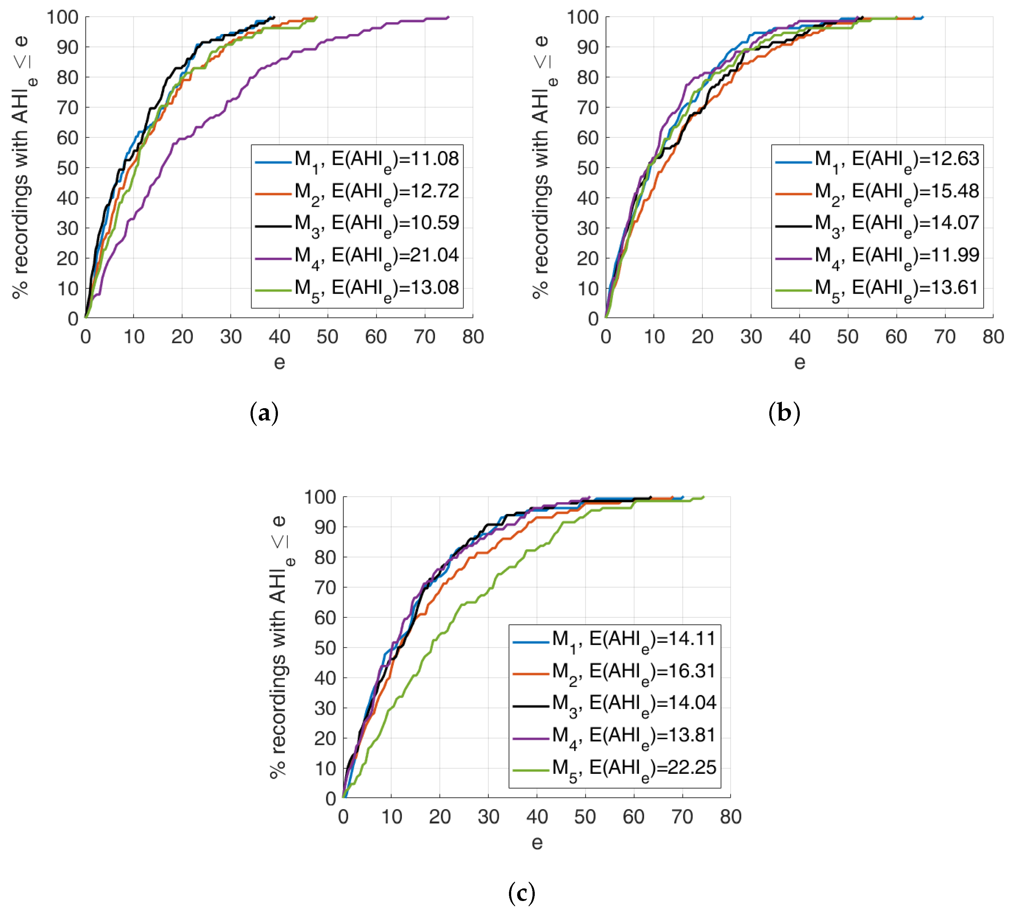
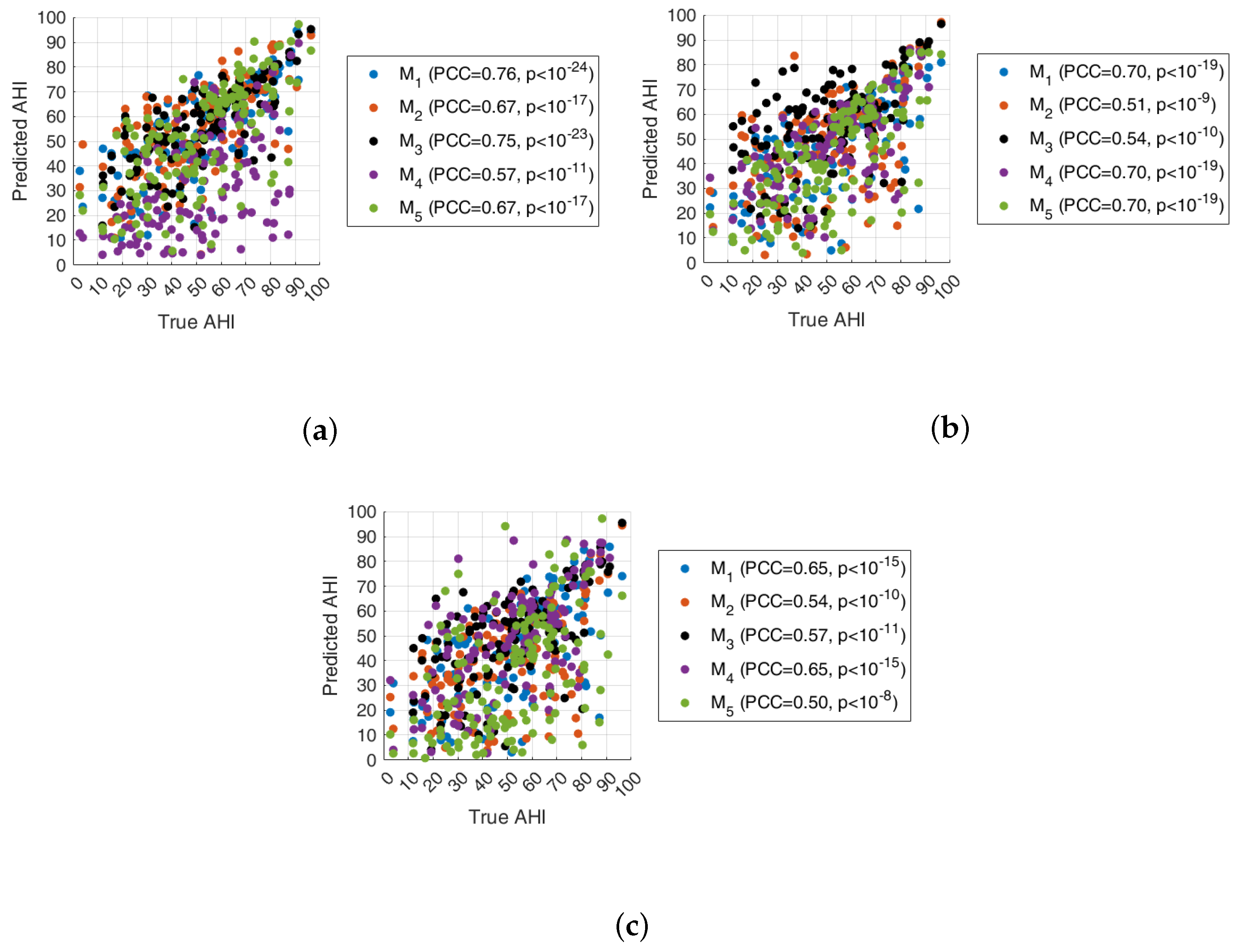
5.2. AHI Estimation and Classification

Encouraged by the results obtained, we tried to verify the ability of the system to predict the AHI value using patients’ recordings over a whole night. An “Apnea”/“Hypopnea” event only needs to be reported if the apnea lasts for a certain time. To detect these types of events by analyzing the patient recordings, we consider a sliding window of 5 s duration moving at a step of 1 s. At each step, we process the sound samples within the window to obtain a sequence of 17 mel spectrograms, which is used as input to the VGGish network. The output of the VGGish network at the “pool4” layer will be a sequence of 17 arrays. This last sequence will be the input for the trained bi-LSTM networks. Accordingly, the outputs of these networks are generated every 1 s and consist of the predicted values for the classes “IN” and “OUT”. These two prediction values are in the range of 0 to 1 and an output value next to 1 means a strong prediction of class membership. Conversely, values approaching 0 indicate a poor prediction of class membership. We evaluated the difference $d=IN-OUT$ (in the range $-1,\dots ,1$) between the two outputs of the architecture depicted in Figure 6.

The evaluation of d for each subsequent sliding window allows us to obtain a curve $d\left(t\right)$ where values approaching $-1$ denote “No-Apnea” conditions, while values approaching 1 denote “Apnea/Hypopnea” conditions. To smooth the trend of these curves, we evaluate the median value in a sliding window of 17 elements corresponding to the size of the audio processing window. The smoothed value is denoted as $\widehat{d}\left(t\right)$. Figure 7 shows an example of the trend of $\widehat{d}\left(t\right)$ for a time interval of half an hour.

In our study, we adopt a methodological approach that utilizes two thresholds, $T{h}_1$ and $T{h}_2$, to identify and classify “Apnea/Hypopnea” events from sleep recordings. Specifically, an interval of time is classified as an “Apnea/Hypopnea” event when the smoothed value $\widehat{d}\left(t\right)$ remains above $T{h}_1$ for a minimum duration specified by $T{h}_2$. This criterion ensures robust event detection by requiring sustained deviations indicative of respiratory disturbance. In addition, OSAHS patients are medically categorized into four levels: normal ($AHI<5$), mild ($5\le AHI<15$), moderate ($15\le AHI<30$), and severe ($30\le AHI$). Accordingly, we can consider the classification performance of our models with respect to these classes.

Unfortunately, our dataset exhibits a significant imbalance across these severity classes, as depicted in

Table 5. Distribution of recordings in the various folds according to the AHI classes.

AHI Class	F #1	F #2	F #3	F #4	F #5	F #6	ALL
Normal	0	0	2	0	0	0	$\mathbf{2}$
Mild	0	2	0	1	0	1	$\mathbf{4}$
Moderate	4	4	5	5	5	2	$\mathbf{25}$
Severe	28	26	25	26	27	29	$\mathbf{161}$

, which presents challenges in model training and evaluation. To address this issue, we employ Bayesian optimization to define optimal values for $T{h}_1$ and $T{h}_2$. This optimization strategy aims to enhance the sensitivity and specificity of our event detection method, thereby improving the accuracy of OSAHS classification.

We used the $N_F=32$ records from patients in fold #6, which were never used to train and test the models. We called $AH{I}_T\left(r\right)$ the true AHI for recording r and $AH{I}_P\left(r\right)$ the predicted AHI for the same recording and considered three different objective functions:

• The absolute value of the AHI error averaged over all recordings

  $$O_A=\frac{{\sum }_{r=1}^{N_F}AH{I}_e\left(r\right)}{N_F};$$

  (1)
• The relative absolute value of the AHI error, averaged over all recordings

  $$O_R=\frac{{\sum }_{r=1}^{N_F}\frac{AH{I}_e\left(r\right)}{AH{I}_T\left(r\right)}}{N_F};$$

  (2)
• The class-weighted absolute value of the AHI error, averaged over all recordings

  $$O_{CA}=\sum _{r=1}^{N_F}\frac{AH{I}_e\left(r\right)}{N_x\left(r\right)};$$

  (3)

where $AH{I}_e\left(r\right)=|AH{I}_T\left(r\right)-AH{I}_P\left(r\right)|$ is the absolute error in estimating the AHI for the processed recording r and $N_x\left(r\right)$ is equal to the number of recordings in the fold that have the same class of recording r.

The objective function in Equation (2) takes into account that equal absolute errors are not of equal importance due to the different amplitudes of the AHI intervals used to define the classes. The objective function in Equation (3) aims to compensate for the unbalanced distribution of recordings in each class of the dataset. We searched for the optimal values of the two thresholds $T{h}_1$ and $T{h}_2$ for each of the five models. Figure 8 shows, as an example, the results of the objective function and the corresponding optimal pairs of thresholds ($T{h}_1$, $T{h}_2$) evaluated with the model $M_3$ and the three objective functions considered.

Table 6. Thresholds to evaluate AHI from $\widehat{d}\left(t\right)$ evaluated with bayesopt Matlab function for the three different objective functions and five models.

	${\mathit{O}}_{\mathit{A}}$		${\mathit{O}}_{\mathit{R}}$		${\mathit{O}}_{\mathit{CA}}$
	${\mathit{Th}}_{\mathbf{1}}$	${\mathit{Th}}_{\mathbf{2}}$	${\mathit{Th}}_{\mathbf{1}}$	${\mathit{Th}}_{\mathbf{2}}$	${\mathit{Th}}_{\mathbf{1}}$	${\mathit{Th}}_{\mathbf{2}}$
$M_1$	$-0.9290$	49	$-0.9751$	62	$-0.9788$	59
$M_2$	$-0.9502$	47	$-0.7731$	50	$-0.8635$	66
$M_3$	$-0.9136$	50	$-0.6154$	37	$-0.6508$	47
$M_4$	$-0.9898$	47	$-0.9344$	58	$-0.2697$	25
$M_5$	$-0.9764$	47	$-0.9344$	58	$-0.9857$	35

shows the thresholds obtained by applying Bayesian optimization to each model according to the three proposed objective functions.

To evaluate the performance of each model, we processed the corresponding output ${\widehat{d}}_{M_i,r}\left(t\right)$ and applied the corresponding pair of thresholds ($T{h}_{1,M_i},T{h}_{2,M_i}$) for each recording $r\in \overline{{\mathcal{R}}_i}$ to obtain the predicted $AH{I}_p\left(r\right)$. $\overline{{\mathcal{R}}_i}$ is the complementary set of ${\mathcal{R}}_i$ containing the 32 recordings used to train the model $M_i$ (Table 2). Accordingly, the number of recordings used to test each model is equal to 128.

Figure 9 shows curves related to the percentage of recordings that have an $AH{I}_e\le e$ for each model considering the different objective functions.

The results obtained with the different models are quite overlapping, except $M_4$ for the objective function $O_A$ and $M_5$ for the objective function $O_{CA}$. In general, about $50\%$ of the tested recordings show an $AH{I}_e\le 10$.

The scatter plots (Figure 10) illustrate a good correlation between the true AHI and the predicted AHI value. The Pearson correlation coefficient (PCC) assumes a larger value for thresholds optimized with the objective function $O_A$. The associated p-value is always very small.

However, it is necessary to evaluate the result of the classification because the same absolute error may or may not produce an error depending on the distance from the boundaries. Figure 11 shows the confusion matrices obtained by processing the recordings for each model and for each threshold optimization approach. If we analyze the mapping column by column, we can show the behavior of the models using the same optimization approach. For example, the high number of bad classifications when using the model $M_4$ with the optimization approach $O_A$ (Figure 11j) and using the model $M_5$ with the optimization approach $O_{CA}$ reflects the results in $AH{I}_e$ obtained for the model $M_4$ in Figure 9a and for the model $M_5$ in Figure 9c.

Analyzing the rows of Figure 11, it is possible to infer how the different objective functions influence the classification performance. The $O_A$ approach allows us to obtain a higher number of correct classifications for “Severe” conditions, but the other classes are generally overestimated. This effect is partially reduced with the $O_R$ and $O_{CA}$ approaches, but the number of underestimations for the “Severe” class increases.

With the aim of presenting the results in a compact way, we analyzed the percentage of correctly estimated, overestimated, and underestimated recordings. Accordingly, starting from a general confusion matrix $\mathbf{C}$, we evaluated

$$\begin{array}{cccc}\hfill & E_R=\frac{{\sum }_{i=1}^{N_c}{\mathbf{C}}_{i,i}}{{\sum }_{i=1,j=1}^{N_c}{\mathbf{C}}_{i,j}}\hfill & \hfill E_O=\frac{{\sum }_{i=1,j=i+1}^{N_c}{\mathbf{C}}_{i,j}}{{\sum }_{i=1,j=1}^{N_c}{\mathbf{C}}_{i,j}}& E_U=\frac{{\sum }_{j=1,i=j+1}^{N_c}{\mathbf{C}}_{i,j}}{{\sum }_{i=1,j=1}^{N_c}{\mathbf{C}}_{i,j}}\hfill \end{array}$$

(4)

where $N_c$ is the number of classes.

Table 7. Percentage of right estimation $E_R$, underestimation $E_U$, and overestimation $E_O$ for the three different objective functions and five models.

	${\mathit{O}}_{\mathit{A}}$			${\mathit{O}}_{\mathit{R}}$			${\mathit{O}}_{\mathit{CA}}$
	${\mathit{E}}_{\mathit{R}}\mathbf{(}\mathbf{\%}\mathbf{)}$	${\mathit{E}}_{\mathit{O}}\mathbf{(}\mathbf{\%}\mathbf{)}$	${\mathit{E}}_{\mathit{U}}\mathbf{(}\mathbf{\%}\mathbf{)}$	${\mathit{E}}_{\mathit{R}}\mathbf{(}\mathbf{\%}\mathbf{)}$	${\mathit{E}}_{\mathit{O}}\mathbf{(}\mathbf{\%}\mathbf{)}$	${\mathit{E}}_{\mathit{U}}\mathbf{(}\mathbf{\%}\mathbf{)}$	${\mathit{E}}_{\mathit{R}}\mathbf{(}\mathbf{\%}\mathbf{)}$	${\mathit{E}}_{\mathit{O}}\mathbf{(}\mathbf{\%}\mathbf{)}$	${\mathit{E}}_{\mathit{U}}\mathbf{(}\mathbf{\%}\mathbf{)}$
$M_1$	$82.81$	$12.50$	$4.69$	$75.78$	$10.94$	$13.28$	$71.09$	$11.72$	$17.19$
$M_2$	$\mathbf{84}.\mathbf{38}$	$11.72$	$\mathbf{3}.\mathbf{91}$	$73.44$	$11.72$	$14.84$	$71.09$	$9.38$	$19.53$
$M_3$	$83.59$	$12.50$	$\mathbf{3}.\mathbf{91}$	$\mathbf{81}.\mathbf{25}$	$12.50$	$\mathbf{6}.\mathbf{25}$	$74.22$	$11.72$	$\mathbf{14}.\mathbf{06}$
$M_4$	$53.12$	$\mathbf{2}.\mathbf{34}$	$44.53$	$76.56$	$11.72$	$11.72$	$\mathbf{75}.\mathbf{78}$	$7.81$	$16.41$
$M_5$	$76.56$	$10.94$	$12.50$	$68.75$	$\mathbf{9}.\mathbf{38}$	$21.88$	$53.91$	$\mathbf{7}.\mathbf{03}$	$39.06$

shows the results obtained for the three different objective functions and five models.

The best results in terms of correct estimation are obtained with the $O_A$ approach and, in particular, $M_2$ provides the higher value of $84.38\%$. From a medical point of view, it seems important to keep the underestimation rate low as it corresponds to sick patients classified as healthy. Excluding the $M_4$ model, the $O_A$ approach shows better results ($3.91\%$ for the $M_2$ and $M_3$ models), while $O_{CA}$ shows the worst performance with the lowest value of $14.06\%$ for the $M_3$ model.

The previous results can be further improved by using a weighting matrix to give different weights to the type of misclassification. Accordingly, it is possible to consider the modified performance parameters:

$$\begin{array}{cccc}\hfill & E_R^{\prime }=\frac{{\sum }_{i=1}^{N_c}{\mathbf{A}}_{i,i}{\mathbf{C}}_{i,i}}{{\sum }_{i=1,j=1}^{N_c}{\mathbf{A}}_{i,j}{\mathbf{C}}_{i,j}}\hfill & \hfill E_O^{\prime }=\frac{{\sum }_{i=1,j=i+1}^{N_c}{\mathbf{A}}_{i,j}{\mathbf{C}}_{i,j}}{{\sum }_{i=1,j=1}^{N_c}{\mathbf{A}}_{i,j}{\mathbf{C}}_{i,j}}& E_U^{\prime }=\frac{{\sum }_{j=1,i=j+1}^{N_c}{\mathbf{A}}_{i,j}{\mathbf{C}}_{i,j}}{{\sum }_{i=1,j=1}^{N_c}{\mathbf{A}}_{i,j}{\mathbf{C}}_{i,j}}\hfill \end{array}$$

(5)

where A is specifically built to weight the type of misclassification. We consider an A-matrix that weights the misclassification depending on the “distance” to the correct class. Accordingly, the weighting for the same class is equal to 1, the weighting for two neighboring classes is equal to 2 (“Normal”–“Mild”, “Mild”–“Moderate”, “Moderate”–“Severe”), and so on:

$$A=\left[\begin{array}{cccc}1& 2& 3& 4\\ 2& 1& 2& 3\\ 3& 2& 1& 2\\ 4& 3& 2& 1\end{array}\right]$$

(6)

Table 8. Percentage of weighted correct estimation $E_R^{\prime }$, underestimation $E_U^{\prime }$, and overestimation $E_O^{\prime }$ for the three different objective functions and five models.

	${\mathit{O}}_{\mathit{A}}$			${\mathit{O}}_{\mathit{R}}$			${\mathit{O}}_{\mathit{CA}}$
	${\mathit{E}}_{\mathit{R}}^{\mathbf{\prime }}\mathbf{(}\mathbf{\%}\mathbf{)}$	${\mathit{E}}_{\mathit{O}}^{\mathbf{\prime }}\mathbf{(}\mathbf{\%}\mathbf{)}$	${\mathit{E}}_{\mathit{U}}^{\mathbf{\prime }}\mathbf{(}\mathbf{\%}\mathbf{)}$	${\mathit{E}}_{\mathit{R}}^{\mathbf{\prime }}\mathbf{(}\mathbf{\%}\mathbf{)}$	${\mathit{E}}_{\mathit{O}}^{\mathbf{\prime }}\mathbf{(}\mathbf{\%}\mathbf{)}$	${\mathit{E}}_{\mathit{U}}^{\mathbf{\prime }}\mathbf{(}\mathbf{\%}\mathbf{)}$	${\mathit{E}}_{\mathit{R}}^{\mathbf{\prime }}\mathbf{(}\mathbf{\%}\mathbf{)}$	${\mathit{E}}_{\mathit{O}}^{\mathbf{\prime }}\mathbf{(}\mathbf{\%}\mathbf{)}$	${\mathit{E}}_{\mathit{U}}^{\mathbf{\prime }}\mathbf{(}\mathbf{\%}\mathbf{)}$
$M_1$	$67.95$	$23.72$	$8.33$	$58.08$	$17.96$	$23.95$	$52.30$	$18.97$	$28.74$
$M_2$	$69.68$	$22.58$	$7.74$	$54.65$	$18.60$	$26.74$	$51.12$	$14.61$	$34.27$
$M_3$	$\mathbf{70}.\mathbf{86}$	$22.52$	$\mathbf{6}.\mathbf{62}$	$\mathbf{66}.\mathbf{24}$	$22.29$	$\mathbf{11}.\mathbf{46}$	$55.88$	$18.24$	$\mathbf{25}.\mathbf{88}$
$M_4$	$32.54$	$\mathbf{2}.\mathbf{87}$	$64.59$	$60.12$	$19.63$	$20.25$	$\mathbf{58}.\mathbf{08}$	$13.17$	$28.74$
$M_5$	$59.76$	$18.90$	$21.34$	$49.16$	$\mathbf{13}.\mathbf{97}$	$36.87$	$32.24$	$\mathbf{8}.\mathbf{41}$	$59.35$

shows the results obtained for the three different objective functions and five models, taking into account the weighted errors. The $O_A$ approach continues to give the best performance, especially for the $M_3$ model. Other A matrices can also be used, for example, to emphasize the overestimation with respect to the underestimation.

Discussion

We base our discussion on the same paper that we analyzed in Section 5.1.1. In [28], no AHI estimation and/or AHI severity prediction was analyzed. In [30], the AHI was estimated based on the detected apnea–hypopnea snoring sounds and yielded a PCC of $0.966$ (p-value $<0.001$). This result was obtained by selecting the snoring sounds of 39 subjects in the training set and the snoring sound of 1 subject as the test set. The process was repeated 40 times to calculate the average metrics. The authors showed the results only as a scatter plot; the prediction of AHI severity cannot be analyzed further. In [29], the AHI determined in the experiment and measured by PSG had a PCC of $0.913$ (p-value $<0.001$). This result was obtained by analyzing the snoring sounds of 10 subjects who did not participate in the training phase. The results in terms of AHI severity classification appear to be good, with a detection rate of $90\%$ (only one subject’s AHI severity was misclassified from “Moderate” to “Mild”). However, it should be noted that the recordings tested do not include “Mild” and “Normal” AHI severity grades. In addition, the number of recordings tested is very small, so that the statistical significance of the result appears questionable.

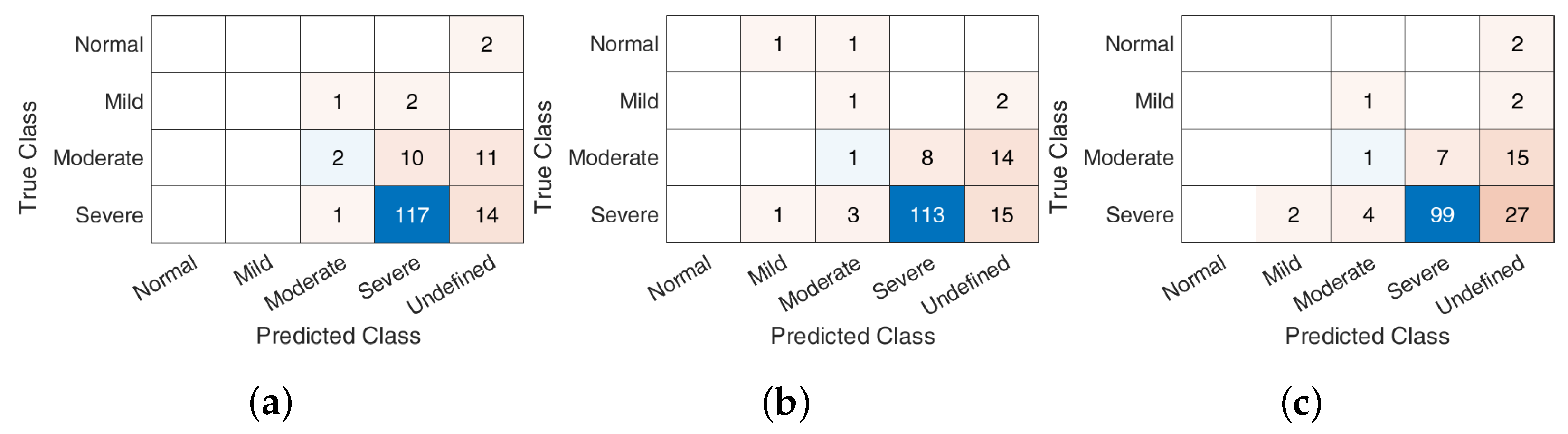
5.3. Models Aggregation

As a final experiment, we propose the classification of AHI severity by aggregation of models. To classify a particular recording, it is possible to use the results of each individual model and create a unique classification by aggregating the results. The recordings $r\in {\mathcal{R}}_i$ are processed with the models $M_j,j=1,\dots ,5:j\ne i$; accordingly, each recording is processed with four different models. To perform the aggregate classification, we analyzed the class predicted by each model for the recordings r, $P_j\left(r\right)$, and counted the results for each class:

$$C{P}_{class}\left(r\right)=\sum _{j=1}^4{P}_j\left(r\right)==class$$

(7)

where $class\in \{\mathrm{Normal},\mathrm{Mild},\mathrm{Moderate},\mathrm{Severe}\}$. Specifically, we chose two different approaches:

• ${\mathcal{P}}_1$:

  $$\widehat{P}\left(r\right)=\left\{\begin{array}{cc}class\hfill & \mathrm{if}C{P}_{class}\left(r\right)>C{P}_{clas{s}^{\prime }}\left(r\right)\forall clas{s}^{\prime }\ne class\hfill \\ undefined\hfill & \mathrm{otherwise}\hfill \end{array}\right.$$

  (8)
• ${\mathcal{P}}_2$:

  $$\widehat{P}\left(r\right)=\left\{\begin{array}{cc}class\hfill & \mathrm{if}\exists class:C{P}_{class}\left(r\right)>2\hfill \\ undefined\hfill & \mathrm{otherwise}\hfill \end{array}\right.$$

  (9)

where $\widehat{P}\left(r\right)$ is the aggregated predicted class. We introduced the $undefined$ result to not assign a class when the predictions of the models are not coherent. More precisely, the policy ${\mathcal{P}}_1$ assigns the $class$ to the aggregated prediction if the number of models predicting the $class$ exceeds all others (for example, $(C{P}_{normal}\left(r\right)=1,C{P}_{mild}\left(r\right)=0,C{P}_{moderate}\left(r\right)=1,C{P}_{severe}\left(r\right)=2)\Rightarrow \widehat{P}\left(r\right)=severe$, $(C{P}_{normal}\left(r\right)=2,C{P}_{mild}\left(r\right)=0,C{P}_{moderate}\left(r\right)=2,C{P}_{severe}\left(r\right)=0)\Rightarrow \widehat{P}\left(r\right)=undefined$); policy ${\mathcal{P}}_2$ assigns $class$ to the aggregated prediction if the number of models predicting $class$ is at least half plus one of all models (for example, $(C{P}_{normal}\left(r\right)=1,C{P}_{mild}\left(r\right)=0,C{P}_{moderate}\left(r\right)=1,C{P}_{severe}\left(r\right)=2)\Rightarrow \widehat{P}\left(r\right)=undefined$, $(C{P}_{normal}\left(r\right)=2,C{P}_{mild}\left(r\right)=0,C{P}_{moderate}\left(r\right)=2,C{P}_{severe}\left(r\right)=0)\Rightarrow \widehat{P}\left(r\right)=undefined$, $(C{P}_{normal}\left(r\right)=0,C{P}_{mild}\left(r\right)=3,C{P}_{moderate}\left(r\right)=1,C{P}_{severe}\left(r\right)=0)\Rightarrow \widehat{P}\left(r\right)=mild$).

Figure 12 and Figure 13 show the confusion matrices obtained with the two different strategies, respectively. We analyzed the results using all the proposed approaches to set the threshold pair $(T{h}_1,T{h}_2)$ to evaluate the AHI. For both strategies, the number of undefined recordings is the lowest when the thresholds are optimized using the $O_A$ approach. As expected, the strategy ${\mathcal{P}}_2$ is more aggressive and classifies more recordings as “undefined” than ${\mathcal{P}}_1$. Differently, the number of underestimated recordings obtained with the strategy ${\mathcal{P}}_2$ is very low and underestimation only occurs in the “Severe” class.

Table 9. Percentage of undefined recordings $E_{ud}$, right estimation $E_R$, underestimation $E_U$, and overestimation $E_O$ for the three different objective function using policy ${\mathcal{P}}_1$ and aggregate model.

	${\mathit{E}}_{\mathit{ud}}(\%)$	${\mathit{E}}_{\mathit{R}}(\%)$	${\mathit{E}}_{\mathit{U}}(\%)$	${\mathit{E}}_{\mathit{O}}(\%)$
$O_A$	$7.50$	$78.75$	$11.25$	$2.50$
$O_R$	$8.75$	$75.62$	$10.62$	$5.00$
$O_{CA}$	$10.00$	$72.50$	$8.75$	$8.75$

and

Table 10. Percentage of undefined recordings $E_{ud}$, right estimation $E_R$, underestimation $E_U$, and overestimation $E_O$ for the three different objective function using policy ${\mathcal{P}}_2$ and aggregate model.

	${\mathit{E}}_{\mathit{ud}}(\%)$	${\mathit{E}}_{\mathit{R}}(\%)$	${\mathit{E}}_{\mathit{U}}(\%)$	${\mathit{E}}_{\mathit{O}}(\%)$
$O_A$	$16.88$	$74.38$	$8.12$	$0.62$
$O_R$	$19.38$	$71.25$	$6.88$	$2.50$
$O_{CA}$	$28.75$	$62.50$	$5.00$	$3.75$

show the performance for aggregate models in terms of undefined severity results ($E_{ud}$), correct severity estimation ($E_R$), underestimation of severity ($E_U$), and overestimation of severity ($E_O$) for the aggregate model and policy ${\mathcal{P}}_1$ and ${\mathcal{P}}_2$, respectively. Although the best performance is obtained with the ${\mathcal{P}}_1$ policy and the $O_A$ approach to set thresholds, the results are most conservative when the ${\mathcal{P}}_2$ policy and the $O_{CA}$ approach to set thresholds are used. The percentage of undefined records is high, but the model never returns too-low values for moderate and mild classes. The percentage of “Severe” recordings that are underestimated is $4.55\%$ (Figure 13c). Obviously, the “undefined” recordings can be further processed by doctors to assign the correct AHI class.

6. Conclusions

This study aimed to propose new strategies for the investigation of OSAHS by exploring the use of low-cost and noninvasive audio signals for OSAHS diagnosis. It investigated the identification of OSAHS events, including classification of apnea/non-apnea status, prediction of apnea–hypopnea index (AHI), and classification of AHI severity. We used a dataset consisting of recordings from a recently curated cohort of subjects undergoing diagnosis for sleep apnea syndrome. The proposed approach involves the use of a convolutional neural network based on a VGGish structure in combination with a bidirectional LSTM for sequence classification. The audio signals are processed into mel spectrograms, which are then fed into the CNN to extract high-level features that serve as input to the bi-LSTM. The results show promising performance of the proposed bi-LSTM in combination with the VGGish architecture, outperforming previous approaches in terms of precision, specificity, accuracy, recall, and F1-score. The classification models demonstrated the ability to discriminate between apnea and non-apnea events even when using data from patients who did not participate in the training phase. In addition, the optimal thresholds for apnea/hypopnea event detection and AHI severity classification were determined using Bayesian optimization. The results showed a strong correlation between the predicted and actual AHI values.

Aggregation strategies were also proposed for the developed model using different optimization methods and merging strategies. The results were good in terms of reducing overestimation and underestimation of severity. The presence of undefined cases can be addressed with the help of medical doctors whose effort in labeling the entire dataset is significantly reduced. To summarize, the research presents a promising approach to OSAHS diagnosis using audio signals acquired through low-cost environmental devices, and deep neural networks. The proposed models show robust performance in event classification and AHI estimation and offer a potentially more convenient and scalable alternative to traditional PSG methods. This work opens exciting avenues for future research, including expanding the training data by collecting information from more subjects and also addressing the problem of AHI severity imbalance using data augmentation techniques. In addition, incorporating explainable AI techniques (XAI) can help clinicians trust the results and give patients confidence in the diagnosis. Finally, exploring multimodal data fusion and validating the model in the clinical setting promises a more robust and practical OSAHS diagnostic tool.

References

1. Pavlova, M.K.; Latreille, V. Sleep disorders. Am. J. Med. 2019, 132, 292–299. [Google Scholar] [CrossRef] [PubMed]
2. Armstrong, M.; Wallace, C.; Marais, J. The effect of surgery upon the quality of life in snoring patients and their partners: A between-subjects case-controlled trial. Clin. Otolaryngol. Allied Sci. 1999, 24, 510–522. [Google Scholar] [CrossRef] [PubMed]
3. Gall, R.; Isaac, L.; Kryger, M. Quality of life in mild obstructive sleep apnea. Sleep 1993, 16, S59–S61. [Google Scholar] [CrossRef] [PubMed]
4. Zhu, K.; Li, M.; Akbarian, S.; Hafezi, M.; Yadollahi, A.; Taati, B. Vision-based heart and respiratory rate monitoring during sleep—A validation study for the population at risk of sleep apnea. IEEE J. Transl. Eng. Health Med. 2019, 7, 1900708. [Google Scholar] [CrossRef] [PubMed]
5. Imtiaz, S.A. A systematic review of sensing technologies for wearable sleep staging. Sensors 2021, 21, 1562. [Google Scholar] [CrossRef]
6. Sabil, A.; Glos, M.; Günther, A.; Schöbel, C.; Veauthier, C.; Fietze, I.; Penzel, T. Comparison of apnea detection using oronasal thermal airflow sensor, nasal pressure transducer, respiratory inductance plethysmography and tracheal sound sensor. J. Clin. Sleep Med. 2019, 15, 285–292. [Google Scholar] [CrossRef] [PubMed]
7. Fietze, I.; Laharnar, N.; Obst, A.; Ewert, R.; Felix, S.B.; Garcia, C.; Gläser, S.; Glos, M.; Schmidt, C.O.; Stubbe, B.; et al. Prevalence and association analysis of obstructive sleep apnea with gender and age differences—Results of SHIP-Trend. J. Sleep Res. 2019, 28, e12770. [Google Scholar] [CrossRef]
8. Berry, R.B.; Brooks, R.; Gamaldo, C.E.; Harding, S.M.; Marcus, C.; Vaughn, B.V. The AASM manual for the scoring of sleep and associated events. Rules Terminol. Tech. Specif. Darien Illinois Am. Acad. Sleep Med. 2012, 176, 2012. [Google Scholar]
9. Bhutada, A.M.; Broughton, W.A.; Garand, K.L. Obstructive sleep apnea syndrome (OSAS) and swallowing function—A systematic review. Sleep Breath. 2020, 24, 791–799. [Google Scholar] [CrossRef]
10. Almazaydeh, L.; Elleithy, K.; Faezipour, M. Obstructive sleep apnea detection using SVM-based classification of ECG signal features. In Proceedings of the 2012 Annual International Conference of the IEEE Engineering in Medicine and Biology Society, San Diego, CA, USA, 28 August–1 September 2012; pp. 4938–4941. [Google Scholar]
11. Mendonca, F.; Mostafa, S.S.; Ravelo-Garcia, A.G.; Morgado-Dias, F.; Penzel, T. A review of obstructive sleep apnea detection approaches. IEEE J. Biomed. Health Inform. 2018, 23, 825–837. [Google Scholar] [CrossRef]
12. Zhou, Q.; Shan, J.; Ding, W.; Wang, C.; Yuan, S.; Sun, F.; Li, H.; Fang, B. Cough Recognition Based on Mel-Spectrogram and Convolutional Neural Network. Front. Robot. AI 2021, 8, 580080. [Google Scholar] [CrossRef] [PubMed]
13. Castro-Ospina, A.E.; Solarte-Sanchez, M.A.; Vega-Escobar, L.S.; Isaza, C.; MartÃnez-Vargas, J.D. Graph-Based Audio Classification Using Pre-Trained Models and Graph Neural Networks. Sensors 2024, 24, 2106. [Google Scholar] [CrossRef] [PubMed]
14. Serrano, S.; Patanè, L.; Scarpa, M. Obstructive Sleep Apnea identification based on VGGish networks. In Proceedings of the Proceedings—European Council for Modelling and Simulation, ECMS, Florence, Italy, 20–23 June 2023; pp. 556–561. [Google Scholar]
15. Korompili, G.; Amfilochiou, A.; Kokkalas, L.; Mitilineos, S.A.; Tatlas, N.A.; Kouvaras, M.; Kastanakis, E.; Maniou, C.; Potirakis, S.M. PSG-Audio, a scored polysomnography dataset with simultaneous audio recordings for sleep apnea studies. Sci. Data 2021, 8, 1–13. [Google Scholar] [CrossRef] [PubMed]
16. Yang, C.; Cheung, G.; Stankovic, V.; Chan, K.; Ono, N. Sleep apnea detection via depth video and audio feature learning. IEEE Trans. Multimed. 2016, 19, 822–835. [Google Scholar] [CrossRef]
17. Amiriparian, S.; Gerczuk, M.; Ottl, S.; Cummins, N.; Freitag, M.; Pugachevskiy, S.; Baird, A.; Schuller, B. Snore sound classification using image-based deep spectrum features. In Proceedings of the INTERSPEECH 2017, Stockholm, Sweden, 20–24 August 2017. [Google Scholar]
18. Dong, Q.; Jiraraksopakun, Y.; Bhatranand, A. Convolutional Neural Network-Based Obstructive Sleep Apnea Identification. In Proceedings of the 2021 IEEE 6th International Conference on Computer and Communication Systems (ICCCS), Chengdu, China, 23–26 April 2021; pp. 424–428. [Google Scholar]
19. Wang, L.; Guo, S.; Huang, W.; Qiao, Y. Places205-vggnet models for scene recognition. arXiv 2015, arXiv:1508.01667. [Google Scholar]
20. Szegedy, C.; Ioffe, S.; Vanhoucke, V.; Alemi, A.A. Inception-v4, inception-resnet and the impact of residual connections on learning. In Proceedings of the Thirty-First AAAI Conference on Artificial Intelligence, San Francisco, CA, USA, 4–9 February 2017. [Google Scholar]
21. Targ, S.; Almeida, D.; Lyman, K. Resnet in resnet: Generalizing residual architectures. arXiv 2016, arXiv:1603.08029. [Google Scholar]
22. Maritsa, A.A.; Ohnishi, A.; Terada, T.; Tsukamoto, M. Audio-based Wearable Multi-Context Recognition System for Apnea Detection. In Proceedings of the 2021 6th International Conference on Intelligent Informatics and Biomedical Sciences (ICIIBMS), Kyushu, Japan, 25–27 November 2021; Volume 6, pp. 266–273. [Google Scholar]
23. Maritsa, A.A.; Ohnishi, A.; Terada, T.; Tsukamoto, M. Apnea and Sleeping-state Recognition by Combination Use of Openair/Contact Microphones. In Proceedings of the INTERACTION 2022; Information Processing Society of Japan (IPSJ): Tokyo, Japan, 2022; pp. 87–96. [Google Scholar]
24. Wang, C.; Peng, J.; Song, L.; Zhang, X. Automatic snoring sounds detection from sleep sounds via multi-features analysis. Australas. Phys. Eng. Sci. Med. 2017, 40, 127–135. [Google Scholar] [CrossRef] [PubMed]
25. Shen, F.; Cheng, S.; Li, Z.; Yue, K.; Li, W.; Dai, L. Detection of snore from OSAHS patients based on deep learning. J. Healthc. Eng. 2020, 2020, 8864863. [Google Scholar] [CrossRef] [PubMed]
26. Wu, D.; Tao, Z.; Wu, Y.; Shen, C.; Xiao, Z.; Zhang, X.; Wu, D.; Zhao, H. Speech endpoint detection in noisy environment using Spectrogram Boundary Factor. In Proceedings of the 2016 9th International Congress on Image and Signal Processing, BioMedical Engineering and Informatics (CISP-BMEI), Datong, China, 15–17 October 2016; pp. 964–968. [Google Scholar] [CrossRef]
27. Cheng, S.; Wang, C.; Yue, K.; Li, R.; Shen, F.; Shuai, W.; Li, W.; Dai, L. Automated sleep apnea detection in snoring signal using long short-term memory neural networks. Biomed. Signal Process. Control 2022, 71, 103238. [Google Scholar] [CrossRef]
28. Sun, X.; Ding, L.; Song, Y.; Peng, J.; Song, L.; Zhang, X. Automatic identifying OSAHS patients and simple snorers based on Gaussian mixture models. Physiol. Meas. 2023, 44, 045003. [Google Scholar] [CrossRef]
29. Song, Y.; Sun, X.; Ding, L.; Peng, J.; Song, L.; Zhang, X. AHI estimation of OSAHS patients based on snoring classification and fusion model. Am. J. Otolaryngol. 2023, 44, 103964. [Google Scholar] [CrossRef] [PubMed]
30. Ding, L.; Peng, J.; Song, L.; Zhang, X. Automatically detecting apnea-hypopnea snoring signal based on VGG19 + LSTM. Biomed. Signal Process. Control 2023, 80, 104351. [Google Scholar] [CrossRef]
31. SoX-Sound eXchange. Available online: https://sourceforge.net/projects/sox/ (accessed on 29 May 2024).
32. Alzubaidi, L.; Zhang, J.; Humaidi, A.J.; Al-Dujaili, A.; Duan, Y.; Al-Shamma, O.; Santamaría, J.; Fadhel, M.A.; Al-Amidie, M.; Farhan, L. Review of deep learning: Concepts, CNN architectures, challenges, applications, future directions. J. Big Data 2021, 8, 53. [Google Scholar] [CrossRef] [PubMed]
33. Arulkumaran, K.; Deisenroth, M.P.; Brundage, M.; Bharath, A.A. Deep reinforcement learning: A brief survey. IEEE Signal Process. Mag. 2017, 34, 26–38. [Google Scholar] [CrossRef]
34. Luong, N.C.; Hoang, D.T.; Gong, S.; Niyato, D.; Wang, P.; Liang, Y.C.; Kim, D.I. Applications of deep reinforcement learning in communications and networking: A survey. IEEE Commun. Surv. Tutor. 2019, 21, 3133–3174. [Google Scholar] [CrossRef]
35. Bkassiny, M.; Li, Y.; Jayaweera, S.K. A survey on machine-learning techniques in cognitive radios. IEEE Commun. Surv. Tutor. 2012, 15, 1136–1159. [Google Scholar] [CrossRef]
36. Serrano, S.; Scarpa, M.; Maali, A.; Soulmani, A.; Boumaaz, N. Random sampling for effective spectrum sensing in cognitive radio time slotted environment. Phys. Commun. 2021, 49, 101482. [Google Scholar] [CrossRef]
37. Bithas, P.S.; Michailidis, E.T.; Nomikos, N.; Vouyioukas, D.; Kanatas, A.G. A survey on machine-learning techniques for UAV-based communications. Sensors 2019, 19, 5170. [Google Scholar] [CrossRef]
38. Grasso, C.; Raftopoulos, R.; Schembra, G.; Serrano, S. H-HOME: A learning framework of federated FANETs to provide edge computing to future delay-constrained IoT systems. Comput. Netw. 2022, 219, 109449. [Google Scholar] [CrossRef]
39. Serrano, S.; Sahbudin, M.A.B.; Chaouch, C.; Scarpa, M. A new fingerprint definition for effective song recognition. Pattern Recognit. Lett. 2022, 160, 135–141. [Google Scholar] [CrossRef]
40. Sahbudin, M.A.B.; Chaouch, C.; Scarpa, M.; Serrano, S. IOT based song recognition for FM radio station broadcasting. In Proceedings of the 2019 7th International Conference on Information and Communication Technology (ICoICT), Kuala Lumpur, Malaysia, 24–26 July 2019; pp. 1–6. [Google Scholar]
41. Sahbudin, M.A.B.; Scarpa, M.; Serrano, S. MongoDB clustering using K-means for real-time song recognition. In Proceedings of the 2019 International Conference on Computing, Networking and Communications (ICNC), Honolulu, HI, USA, 18–21 February 2019; pp. 350–354. [Google Scholar]
42. Serrano, S.; Scarpa, M. Fast and Accurate Song Recognition: An Approach Based on Multi-Index Hashing. In Proceedings of the 2022 International Conference on Software, Telecommunications and Computer Networks (SoftCOM), Split, Croatia, 22–24 September 2022; pp. 1–6. [Google Scholar] [CrossRef]
43. Alharbi, S.; Alrazgan, M.; Alrashed, A.; Alnomasi, T.; Almojel, R.; Alharbi, R.; Alharbi, S.; Alturki, S.; Alshehri, F.; Almojil, M. Automatic speech recognition: Systematic literature review. IEEE Access 2021, 9, 131858–131876. [Google Scholar] [CrossRef]
44. LeCun, Y.; Bengio, Y.; Hinton, G. Deep learning. Nature 2015, 521, 436–444. [Google Scholar] [CrossRef] [PubMed]
45. Hershey, S.; Chaudhuri, S.; Ellis, D.P.W.; Gemmeke, J.F.; Jansen, A.; Moore, C.; Plakal, M.; Platt, D.; Saurous, R.A.; Seybold, B.; et al. CNN Architectures for Large-Scale Audio Classification. In Proceedings of the 2017 IEEE International Conference on Acoustics, Speech and Signal Processing (ICASSP), New Orleans, LA, USA, 5–9 March 2017. [Google Scholar]
46. The MathWorks Inc. MATLAB Version: 23.2.0.2515942 (R2023b) Update 7. Available online: https://www.mathworks.com (accessed on 29 May 2024).
Figure 1. Typical examples of sequences of mel spectrograms extracted for different types of apnea category and in “No-Apnea” state: (a) “Central Apnea”, (b) “Hypopnea”, (c) “Mixed Apnea”, (d) “Obstructive Apnea”, (e) “No-Apnea”. The x-axis and y-axis are the time and frequency of the sound, respectively.
Electronics 13 02567 g001
Figure 2. Block scheme of the proposed method.
Electronics 13 02567 g002
Figure 3. Bi-LSTM architecture optimization: (a) Estimated objective function values versus hyperparameters; (b) Minimum objective function values versus number of function evaluations.
Electronics 13 02567 g003
Figure 4. Training/validation loss and training/validation recall for (a) M 1 , (b) M 2 , (c) M 3 , (d) M 4 , and (e) M 5 model.
Electronics 13 02567 g004
Figure 5. Confusion matrix, class-wise “precisions”, and class-wise “recalls” for (a) M 1 , (b) M 2 , (c) M 3 , (d) M 4 , and (e) M 5 model.
Electronics 13 02567 g005
Figure 6. Flow diagram of the proposed architecture: from the process recordings to the class prediction.
Electronics 13 02567 g006
Figure 7. Typical time evolution of d ^ ( t ) trend. The thresholds T h 1 and T h 2 are also reported.
Electronics 13 02567 g007
Figure 8. Outcome of the considered objective functions and related optimal values of threshold pairs ( T h 1 , T h 2 ) for model M 3 : (a) O A objective function, (b) O R objective function, (c) O C A objective function.
Electronics 13 02567 g008
Figure 9. Curves indicating the percentage of recordings with A H I e e for each model and taking into account (a) O A objective function, (b) O R objective function, and (c) O C A objective function.
Electronics 13 02567 g009
Figure 10. Scatter diagram between true and predicted AHI. The legends report the value of Pearson correlation coefficient (PCC) and related p-value obtained by each model and thresholds optimized by (a) O A objective function, (b) O R objective function, and (c) O C A objective function.
Electronics 13 02567 g010
Figure 11. Confusion matrices obtained to classify OSAHS severity for each model and optimization approach: (a) M 1 , O A ; (b) M 1 , O R ; (c) M 1 , O C A ; (d) M 2 , O A ; (e) M 2 , O R , (f) M 2 , O C A ; (g) M 3 , O A ; (h) M 3 , O R ; (i) M 3 , O C A ; (j) M 4 , O A ; (k) M 4 , O R ; (l) M 4 , O C A ; (m) M 5 , O A ; (n) M 5 , O R ; (o) M 5 , O C A .
Electronics 13 02567 g011
Figure 12. Confusion matrices obtained to classify OSAHS severity using aggregate model results and policy P 1 : thresholds optimized using (a) O A , (b) O R , and (c) O C A .
Electronics 13 02567 g012
Figure 13. Confusion matrices obtained to classify OSAHS severity using aggregate model results and policy P 2 : thresholds optimized using (a) O A , (b) O R , and (c) O C A .
Electronics 13 02567 g013