NLOCL: Noise-Labeled Online Continual Learning

Abstract

Continual learning (CL) from infinite data streams has become a challenge for neural network models in real-world scenarios. Catastrophic forgetting of previous knowledge occurs in this learning setting, and existing supervised CL methods rely excessively on accurately labeled samples. However, the real-world data labels are usually misled by noise, which influences the CL agents and aggravates forgetting. To address this problem, we propose a method named noise-labeled online continual learning (NLOCL), which implements the online CL model with noise-labeled data streams. NLOCL uses an empirical replay strategy to retain crucial examples, separates data streams by small-loss criteria, and includes semi-supervised fine-tuning for labeled and unlabeled samples. Besides, NLOCL combines small loss with class diversity measures and eliminates online memory partitioning. Furthermore, we optimized the experience replay stage to enhance the model performance by retaining significant clean-labeled examples and carefully selecting suitable samples. In the experiment, we designed noise-labeled data streams by injecting noisy labels into multiple datasets and partitioning tasks to simulate infinite data streams realistically. The experimental results demonstrate the superior performance and robust learning capabilities of our proposed method.

1. Introduction

Neural network models have demonstrated significant advantages across various research domains like computer vision, natural language processing, and target detection. They excel in single-task learning and often outperform humans in tasks such as Atari games and object recognition [1,2]. Nevertheless, these models are difficult to adapt to dynamic data streams and multitask learning scenarios. As new tasks come continuously, the neural networks will encounter a notorious problem called “catastrophic forgetting”, also known as the “plasticity–stability” trade-off [3], leading to considerable performance decline on past tasks. Overcoming catastrophic forgetting of previous tasks is crucial for achieving continuous task learning [4].

Continual learning (CL) aims to address the forgetting issue in never-ending data streams. It focuses on adapting to changing data distributions in real-world scenarios and retaining performance on old tasks while learning new tasks [5]. Researchers have extensively investigated CL to alleviate catastrophic forgetting. Compared with other types of methods, replay-based methods, where the neural network model learns previous task data from a limited memory buffer storing a small amount of observed data, have proven highly effective in combating forgetting. Most CL methods learn in a supervised mode and are extremely dependent on the precision of the labels. Recently, SPR [6] argues that, if a pure replay buffer is maintained, significant performance gains can be achieved. Nevertheless, SPR relies on clean samples and discards the potential noisy samples [7].

However, in real-world scenarios, there are various sources of data, and data quality cannot be guaranteed, leading to the presence of erroneous labels or noisy labels (NLs) in data streams. As NLs increase, supervised learning becomes misleading, which impairs the model performance. This issue is exacerbated in the replay-based CL methods since NLs will be replayed from the memory buffer, which leads to more severe catastrophic forgetting.

To address the challenges associated with noise-labeled data in CL, we propose a novel method called noise-labeled online continual learning (NLOCL), which extends the online CL model to effectively handle data streams with NLs. NLOCL employs an empirical replay strategy to retain and prioritize important examples, ensuring the model focuses on high-quality data during training. NLOCL incorporates semi-supervised fine-tuning, leveraging both labeled and unlabeled samples to improve model robustness. A key innovation of NLOCL is the integration of small loss criteria with class diversity measures, which allows the method to maintain diverse and representative samples. Unlike traditional methods, NLOCL eliminates the need for online memory partitioning, simplifying the implementation and reducing computational overhead. Moreover, we have optimized the experience replay stage to improve model performance significantly. By preserving significant clean-labeled examples and carefully selecting appropriate samples for replay, NLOCL ensures that the model continuously learns from the most relevant data, reducing the negative impact of noisy labels.

In the experiments, we simulated noise-labeled data streams by introducing noisy labels into multitask data streams. This setup allows us to rigorously evaluate the effectiveness of NLOCL under conditions that closely resemble real-world scenarios. The experimental results demonstrate the superior performance and robust learning capabilities of our proposed method, especially showcasing its potential for practical applications with noisy and dynamic data streams.

The rest of this paper is organized as follows: Section 2 presents a review of related work. Section 3 is devoted to our proposed NLOCL method. Extensive experiments are conducted in Section 4 to support our claims. We finish the paper with a conclusion in Section 5.

2. Related Work

2.1. Online Continual Learning

Continual learning settings are able to be categorized into the offline setting and the online setting [6,8]. In the offline setting, unrestricted use of all current task data is infeasible in real-world scenarios, which imposes limits on continual learning. Models are constrained by limited memory space for training assistance. Offline memory space should ideally match the size of the current task dataset. In the online setting, various concepts are proposed by different researchers. The online setting refers to the fact that each stream sample can only be used once in model training [9,10], whereas the research in [11] considers that only one or a few samples pass through the data stream at any given moment. The former has similar memory buffer requirements as the offline setting, resulting in unnecessary memory overhead.

2.2. Catastrophic Forgetting

Catastrophic forgetting is a common challenge in CL models. The primary objective is to prevent the neural network from losing information learned from previous tasks, ensuring stable classification performance across continual tasks. Understanding the causes of catastrophic forgetting is crucial in the CL algorithm, with early studies delving into this phenomenon in detail. EWC [12] examines catastrophic forgetting in continual tasks, identifying causes and introducing the EWC algorithm. EWC belongs to the type of regularization-based approaches in CL and prevents parameter drift by penalizing updates that affect old task parameters, ensuring alignment with optimal parameter spaces [12]. When a model learns two tasks sequentially, the abrupt shift in the data distribution upon the arrival of subsequent tasks can lead to catastrophic forgetting. In real-world scenarios with complex and large datasets, as task turnover increases, the network tends to adjust parameters crucial for previous tasks to accommodate new ones, prioritizing “plasticity” over stability. This trade-off increasingly leans towards sacrificing stability for plasticity for the need to adapt to new tasks.

2.3. Replay-Based Methods

The primary methods for studying CL models are replay-based, regularization-based, and parameter-isolation-based methods. Among these, replay-based methods are versatile and adaptable for CL scenarios. They involve storing or generating samples of previous tasks for replay. This section focuses on the former approach. Although it requires more storage space and memory overhead compared to generating pseudo-samples, the latter method introduces challenges in model generation. In particular, the complex tasks increase continuously, affecting the model robustness. Replay-based methods represent a general learning paradigm, exemplified by the basic algorithm in [13].

In addition to storing and replaying real samples, some methods opt to replay relevant information from previous tasks instead of actual samples. For example, GEM proposes using previous task samples in situational memory to compute the feasible domain of the previous tasks. It then projects the gradient of the current task into this domain to prevent the gradient descent direction from exceeding the bounds of the previous task’s feasible domain [14]. A-GEM [15] simplified GEM by converting the optimization problem into estimating a projection in one direction through random selection from the memory buffer. Recent methods like GPM, TRGP, and GCR advocate avoiding direct access to old data to address potential user data privacy concerns associated with traditional empirical replay-based methods [16,17,18]. These methods store each task’s input space during forward propagation, representing feature substrates at each layer of the input network as a set of orthogonal substrates from previous task inputs. Leveraging the unique relationship between the task gradient descent space and the input space, they constrain the direction of subsequent task gradient descent to safeguard important parameter information from significant changes and preserve old knowledge.

In our work, we propose a replay-based method on the data streams with labeled and unlabeled samples, which satisfies the scenario of the data in reality. We overcome catastrophic forgetting in the online continual learning setting and enhance the model performance by the online memory update strategy, which can retain significant clean-labeled examples in the memory buffer.

3. Methodology

3.1. Problem Description

The main task studied in this paper is the problem of online task-free CL. Beginning with the typical scenario of CL classification tasks, many replay-based CL paradigms have shown good performance, which are still followed in this paper. Assuming a set of n different tasks $t\in \{T_1,T_2,\dots ,T_n\}$, each task’s data distribution is denoted by $D_i$, representing the task index. The model observes a data stream that can undergo abrupt changes from $D_k$ to $D_k+1$, but the model is unaware of the time of the abrupt change in the data distribution. The data seen by the model at a certain time t from the data stream is represented as $X_t$, and in a noisy environment, $Y_t$ is the noisy label. Notably, the representation of samples differs greatly between settings with and without tasks. In both task-free and task-aware settings, the representation of samples differs significantly. In the task-aware setting, the general form of a sample at any given time is represented as $(X_t^i,Y_t^i)$ or $(X_t,Y_t,i)$, where the task identifier i is visible to the neural network. This information helps predict the model output. The minimization of the optimization objective can be represented as:

$$mi{n}_{\theta }\left[L(f(X_D,\theta ),Y_D)+L(f(X_B,\theta ),Y_B)\right],$$

(1)

where L is the corresponding loss function. Due to the adoption of a replay-based approach in this paper, a replay buffer B is maintained for the model. $\{X_D,Y_D\}$ and $\{X_B,Y_B\}$ represent mini-batches from the online data stream, and the replay buffer during fine-tuning is denoted by BB. The loss function integrates values from both the memory buffer and online data streams, forming the basis for learning with noisy labels. This highlights the model’s capacity to assimilate new knowledge while preserving old task information. Replay-based methods naturally excel in retaining previous model knowledge, as demonstrated by this formulation.

CL algorithms in training mode settings can be categorized into class incremental and task incremental [19], also known as task-agnostic and task-aware learning. The distinction between these lies in the use of task identifiers. In task-aware learning, task identifiers are visible to the model during training and testing, aiding in clarifying task boundaries. During training, only the classifier head corresponding to the updated task identifier is selected, while during testing, only the relevant classifier head is activated for prediction. In contrast, task-agnostic learning requires all classifier heads to participate in training and prediction output. The difference between them is reflected in the structure of the model output layer. In task-based CL [20,21,22], each new task requires an additional output head, extending the model’s output layer to accommodate specific task predictions. In contrast, task-agnostic learning keeps all classifier heads fixed during both training and testing stages [23]. There is a more illustrative description of the differences between these two settings in Figure 1.

In [24], it was explicitly pointed out that noisy labels can lead to retrogressive forgetting consequences [25]. In the context of CL, the negative impact of noisy labels lies in disrupting the high-quality memory buffer, leading to more severe catastrophic forgetting phenomena [26,27], which hinders subsequent task learning. The study [24] finds that a clean buffer can help improve performance. Conducting CL in a noisy environment is entirely reasonable based on replay-based methods.

3.2. Overview of Our Method

Figure 1 succinctly outlines our approach, depicting the model’s learning process on the current task data stream online. Initially, the upper section illustrates the scenario of online noisy label learning tasks. Data continually arrive as time progresses, potentially containing noisy labels for each task. At task boundaries, the data distribution may abruptly change. The online data stream initially fills a finite-capacity online buffer. Subsequently, samples from the buffer are categorized into clean-labeled and noise-labeled samples, and eligible samples for inclusion in the global replay buffer are selected. These replay samples along with online samples from future tasks are then utilized for fine-tuning. To maximize the utilization of the online data stream and enhance learning by capturing crucial information, our approach forgoes the constraint of exclusively using clean samples for training.

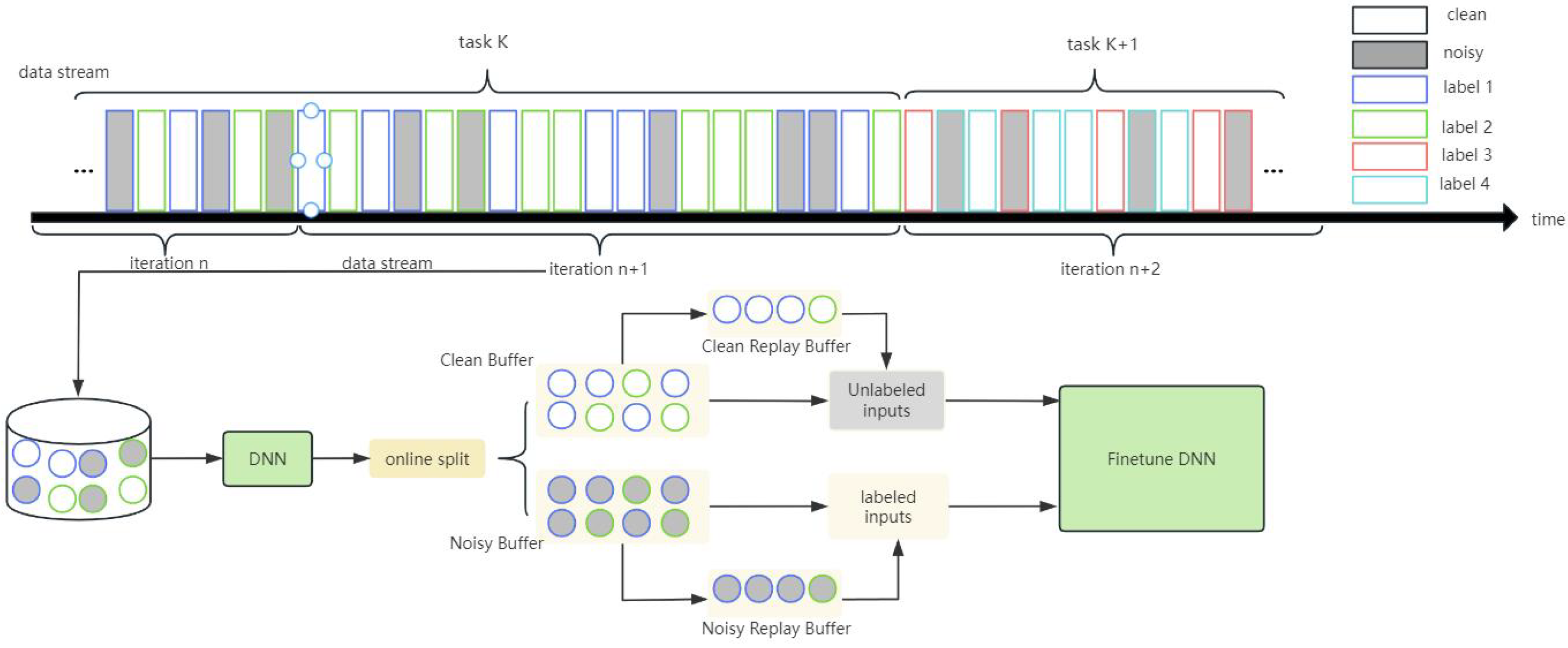
3.3. Online Buffer Separation and Important Example Retaining

The process of dividing the online data stream determines the quality of the labeled data and unlabeled data involved in fine-tuning. Following the paradigm of online CL, a fixed number of samples are taken from the data stream each time, which constitutes an online iteration. The model is represented as $f(;\theta )$. During each iteration, the network engages in supervised learning with a minimal learning rate. Initially, the DNN tends to grasp simple patterns, gradually memorizing noisy labels. Samples with clean labels with minimal losses are prioritized for memorization by the neural network. To differentiate between high-confidence samples and noisy ones, threshold hyperparameters can be configured.

Due to the task-agnostic setting, assuming a total of c classes need to be learned, it means the model always maintains c classifier heads, and all classifier heads participate in the prediction output of each sample. The prediction vector of sample $x_i$ can be represented as $\mathbf{p}=[p_i^1,p_i^2,\cdots ,p_i^c]$. Correspondingly, the label can be represented as $\mathbf{y}=[y_i^1,y_i^2,\cdots ,y_i^c]$. This paper computes the distance between them to describe their difference:

$$L_i=\frac{1}{2}\sum _{j=1}^c{∥y_i^j-p_i^j∥}_2^2.$$

(2)

Due to the characteristics of class incremental learning, $p_i$ can contain classes that the model has not yet learned, which is incorrect. It is necessary to filter out the classes that will only appear in the future from $p_i$ to assist the model in making as accurate judgments as possible in classifying noise. The prediction accuracy might be enhanced by employing a class-specific binary mask. In this approach, the mask distinguishes between previously learned and newly introduced classes. Specifically, it assigns a value of 1 to positions corresponding to both old and current classes, signifying the recognition of these classes, while positions corresponding to yet-to-be-learned classes are set to 0. Solely setting bits related to current task labels to 1 is not exhaustive in capturing the model’s evolving comprehension. Consider a common scenario: the classes contained in task t may correspond to the labels of previous tasks, and the mask bits corresponding to previous task labels will be set to 0. In our approach, we allow predictions of samples to point to labels contained in previous tasks, avoiding the erroneous auxiliary effect of the mask. The mask bit for class j of $x_i$ is represented as $m_i^j$. The formula for calculating the distance of samples with the addition of the corrected mask, which is the mean-squared error loss, is described as follows:

$$L_i=\frac{1}{2}\sum _{j=1}^c{∥y_i^j-m_i^j\otimes p_i^j∥}_2^2.$$

(3)

Compare the distances of all samples in each iteration; mark the samples with distances smaller than the threshold as clean-labeled samples; fill the online buffer with clean samples. Therefore, other samples with larger distances are filled into the buffer for noisy samples as follows:

$${OB}_{clean}\leftarrow \left\{\left(x_i,y_i\right)|\forall L_i<L_{threshold}\right\},$$

(4)

$${OB}_{noisy}\leftarrow \left\{\left(x_i,y_i\right)|\forall L_i>L_{threshold}\right\}.$$

(5)

For the threshold in the above formula, this paper uses the average distance of all samples in the batch to identify as follows:

$$L_{threshold}=\frac{1}{N_{iteration}}\sum _{i=1}^N{L}_i.$$

(6)

From the online buffer of clean samples, select the smallest $N_1$ samples based on the distance, and add them to the replay buffer of clean samples. Correspondingly, select the largest $N_2$ samples based on the distance, and add them to the replay buffer of noisy samples. $N_1$ and $N_2$ are treated as hyperparameters.

The above content describes the process of online sample partitioning and sample selection. There are limitations to existing methods related to noisy label learning, such as SPR [6], which advocates learning feature representations on reliable samples. However, in noisy environments, the limited number of clean samples restricts the model from fully learning the feature representations of each class. Subsequent experiments will also demonstrate the necessity of replaying noisy samples.

3.4. Clean Label Learning

Clean-labeled samples are limited. Despite filtering out the most reliable samples from the online data stream, the network may memorize some noise samples due to the memory effect of deep neural networks, leading to inevitable interference. To enhance the generalization ability and robustness of deep neural networks, the learning of labeled samples introduces a modified data augmentation method called MixUp [27], which generates new examples and labels through linear interpolation. Assume $\{x_{ai},y_{ai}\}$ and $\{x_{bi},y_{bi}\}$ are two data augmentations of an example $\{x_i,y_i\}$, along with their one-hot encoded labels. This results in the MixUp augmentation $\{{\tilde{x}}_i,{\tilde{y}}_i\}$. This method of data augmentation effectively introduces prior knowledge [11] to the network, enhancing its generalization ability, as shown in Figure 2, and the process is shown in the following formula:

$${\tilde{x}}_i=\lambda x_{ai}+{\left(1-\lambda \right)x}_{bi},$$

(7)

$${\tilde{y}}_i=\lambda y_{ai}+{\left(1-\lambda \right)y}_{bi}.$$

(8)

To learn from clean label images, no additional auxiliary learning measures are needed. The augmented samples mentioned above are fed into Net 1, and the corresponding cross-entropy loss referred to as the loss on-labeled samples is computed using the predicted $\tilde{p}$. As shown in Equation (9), N represents the number of input clean-labeled samples, ${\tilde{y}}_i$ represents the label of the ith sample, and ${\tilde{p}}_i$ represents the prediction corresponding to the ith sample by Net 1.

$$L_x=-\frac{1}{N}\sum _{i=1}^N{\tilde{y}}_{i}log\left({\tilde{p}}_i\right).$$

(9)

3.5. Noisy Label Learning

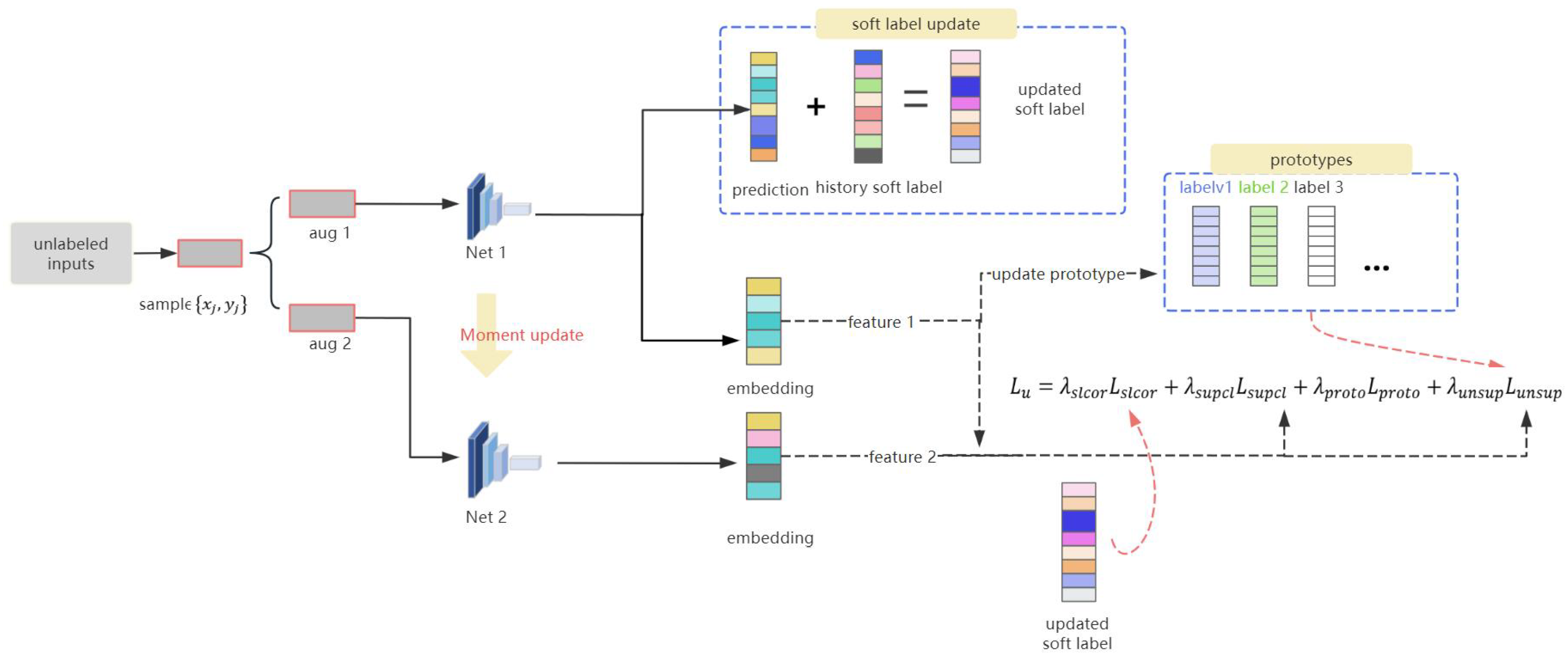
This section shows the fine-tuning framework for learning from noisy labels and entails extracting more information from samples with relatively higher proportions of correctly partitioned noisy labels while minimizing the influence of mislabeled data. Drawing inspiration from the supervised contrastive learning framework SCL2 [28], we optimized its components and introduced a finite memory buffer for caching historical feature representations. Subsequently, we devised a composite loss for unlabeled samples, which integrates unsupervised contrastive learning loss, supervised contrastive learning loss based on soft labels, supervised prototype contrastive learning loss based on soft labels, and corrected soft label loss.

In handling examples with noisy labels, two networks are utilized, denoted in this paper as Net 1 and Net 2. Both networks maintain identical architectures, and Net 1’s parameters are periodically used to perform momentum updates on Net 2’s weights. These momentum updates maintain approximate parameter equality between the two networks while ensuring that the weights of Net 2 change more slowly than those of Net 1, thus preventing Net 1 from being heavily influenced by noise and maintaining model robustness.

For each data example $\{x_i,{\widehat{y}}_i\}$ in the unlabeled sample set U, two different data augmentations are obtained, labeled as $aug\left(x_j\right)$ and $au{g}^{\prime }\left(x_j\right)$. These augmentations, $aug\left(x_j\right)$ and $au{g}^{\prime }\left(x_j\right)$, are, respectively, fed into two models with identical network structures, referred to as Net 1 and Net 2. Net 1 will output the low-dimensional feature embedding of $aug\left(x_j\right)$, denoted as $f(aug\left(x_j\right);\theta )$. In addition to the aforementioned feature embedding, another important output of Net 1 is the prediction regarding the first data augmentation $x_j$, represented as ${\tilde{p}}_j$, which is generated through the fully connected layer of the Net 1. The second data augmentation ${aug}^{\prime }\left(x_j\right)$ is input into Net 2, which only needs to output the low-dimensional feature embedding for this augmented sample, represented as $f(au{g}^{\prime }\left(x_j\right);{\theta }^{\prime })$.

3.6. Loss Function Analysis

The first component of the loss is called soft-label-corrected loss ($L_{slcor}$). The research on noisy label correction [16] proposed the idea of correcting labels using linear interpolation between the original noisy labels and soft labels. The corrected label is represented as $\beta {\widehat{y}}_j+(1-\beta ){\tilde{p}}_j$, where ${\tilde{p}}_j$ represents the network’s output prediction. If the corrected label is used as the supervision signal, the cross-entropy loss can be expressed as follows:

$$L=-\frac{1}{N}\sum _{j=1}^N{\left(\beta {\widehat{y}}_j+\left(1-\beta \right){\tilde{p}}_j\right)}^{T}log{\tilde{p}}_j.$$

(10)

Equation (10) represents the recent network predictions introduced as supervision signals. The short-term memory effect of neural networks prevents using original noisy labels as supervision signals, as the network quickly memorizes some noisy labels, leading to performance degradation. As the number of iterations increases, the influence of the original labels on the network should decrease. The supervision signals are updated with iterations to generate more accurate soft targets. Based on the above discussion, naturally, the updating process of the supervision signals is represented as follows:

$${\tilde{y}}_k=\left\{\begin{array}{cc}\widehat{y}\hfill & \mathrm{if}k=0,\hfill \\ \alpha {\tilde{y}}_{k-1}+(1-\alpha ){\tilde{p}}_j\hfill & \mathrm{if}k>0.\hfill \end{array}\right.$$

(11)

The epoch is represented by k. At any $k>0$-th moment, historical supervision is incorporated into the current supervision update. The update of supervision is summarized as the exponential moving average of historical supervision. The loss of all epochs is divided into the first epoch (first term) and other epochs (second term) as expressed in the following:

$$L_{slcor}=-\sum _{j=1}^N{\alpha }^k{\left({\widehat{y}}_j\right)}^{T}log\left({\tilde{p}}_j\right)-\frac{1}{N}\sum _{j=1}^N\sum _{s=1}^k(1-\alpha ){\alpha }^{k-j}{p}_{j\left[s\right]}^{T}log\left({\tilde{p}}_j\right),$$

(12)

where $p_{j\left[s\right]}$ represents the model’s prediction for $x_j$ in the s-th epoch. Since there are no historical soft labels in the first epoch, the original labels are temporarily used as the supervision. In the first term of the loss, it is weighted by ${\alpha }^k$. $\alpha$ is a real number in the interval $(0,1)$, ensuring that, as the epochs progress, the weight of the original labels in the supervision decreases gradually. The weights of the updated ${\tilde{y}}_k$ increase, especially for the recent ${\tilde{y}}_k$. As the iteration progresses, the model’s predictions become more accurate, which are then used to correct the soft labels more accurately.

The second part of the loss is the supervised contrastive learning loss, denoted as $L_{supcl}$. Given N sample label pairs $\left\{x_j,y_j\right\},j=1,2,\dots ,N$ in a mini-batch, we obtain $2N$ augmented sample pairs $\left\{{\tilde{x}}_s,{\tilde{y}}_s\right\},s=1\dots 2N$ through feature extraction on two networks. Here, ${\tilde{x}}_{2s-1}$ and ${\tilde{x}}_{2s}$ represent two different versions of augmentation for ${\tilde{x}}_s$, and correspondingly, ${\tilde{y}}_s={\tilde{y}}_{2s-1}={\tilde{y}}_{2s}$. Within these $2N$ augmented samples, for any index s representing a sample, $s\in \left\{1\dots 2N\right\}$, we denote the index of a sample that shares the same class label as the s-th sample as t. These two augmented samples are considered positive. The loss for this part is represented as follows:

$$L_{supcl}=\sum _{s=1}^{2N}\frac{-1}{2N_{{\tilde{y}}_s}-1}\sum _{t=1}^{2N}{I}_{s\ne t}{I}_{{\tilde{y}}_s={\tilde{y}}_t}log\frac{exp\left(v_s\raisebox{1ex}{$v_t$}\!\left/ \!\raisebox{-1ex}{$/$}\right.{\tau }_{supcl}\right)}{{\sum }_{k=1}^{2N}{I}_{s\ne k}exp\left(v_s\raisebox{1ex}{$v_k$}\!\left/ \!\raisebox{-1ex}{$/$}\right.{\tau }_{supcl}\right)},$$

(13)

where $v_t$ represents the features of other samples in the same batch as $v_s$, but with the same category as $v_s$. Soft labels are used as supervised information for sample category discrimination. $N_{{\tilde{y}}_s}$ denotes the number of enhanced samples in the batch that have the same category as $v_s$. Using I as the indicator function, its value is 1 when the subscript condition is satisfied; otherwise, it is 0. Clearly, $v_t$ serves as the positive sample for $v_s$, and $v_k$ serves as the negative sample. $\tau$ is the temperature coefficient. When computing $L_{supcl}$, it ensures that positive and negative samples are better distinguished, promoting the network to learn information from features and sample labels from the same category.

The third part of the loss concerns global prototype learning. Maintaining a global prototype matrix provides prototype vectors for class centers, assisting the network in discrimination. The objective is to make the low-dimensional feature representations output by the training network closer to the prototypes of their respective classes. In each subsequent epoch, if the update condition is met, the current prototypes are updated with the exponential moving average of historical prototype vectors and low-dimensional features. This enables the prototypes to evolve as more samples are seen by the model, better characterizing the class centers of each class. The loss formula is shown as follows:

$$c_k=m{c}_k+\left(1-m\right)v_j,\forall j\in \left\{j|{\tilde{y}}_j=k\right\},$$

(14)

where k represents the class label. m denotes the coefficient for the exponential moving average. Here, it is necessary to use supervised information to distinguish the class of prototypes, ensuring that the most correct prototypes are selected for updating. To maintain the stability of prototypes in describing class features, prototype updates can only be performed when two conditions are met. The prototype learning loss function is as follows:

$$L_{proto}=-log\frac{exp\left(v_j{c}_{{\tilde{y}}_j}{\tau }_{proto}\right)}{{\sum }_{k=1}^{K}exp\left(v_j{c}_k{\tau }_{proto}\right)},k\ne c_{{\tilde{y}}_j}.$$

(15)

In the above loss, ${\tilde{y}}_j$ represents the soft label and $\tau$ is the temperature coefficient. There are two prerequisites for prototype updates: first, setting a threshold $\beta$ requires that the aforementioned $L_{proto}$ is less than $\beta$; second, when the sample soft label is the same as the network prediction, meeting this condition restricts the speed of prototype updates and maintaining the stability of the network.

Finally, the completely unsupervised loss function is denoted as $L_{unsup}$. As shown in Figure 3, a small buffer with a queue structure is utilized to store the outputs of Net 2 over a period of time, serving as negative samples. The feature buffer is represented as M, with a capacity limit of $\left|M\right|$. The low-dimensional features of recent online samples in Net 2 are stored in the queue as ${v_j}^{\prime }$. As the queue has limited capacity, this part of the loss is expressed as:

$$L_{unsup}=-log\frac{exp\left(v_j{v_j}^{\prime }{\tau }_{unsup}\right)}{{\sum }_{m=1}^{\left|M\right|}exp\left(v_j{v_m}^{\prime }{\tau }_{unsup}\right)},$$

(16)

where ${v_j}^{\prime }$ represents the feature representation obtained from Net 2 and ${\tau }_{unsup}$ represents the temperature coefficient in this context. ${v_m}^{\prime }$ denotes several historical features in the queue M.

Figure 4 summarizes the learning process of unlabeled samples. It depicts the dual-model structure and indicates momentum updates. The main components of the loss function and the information contained in the model output within the loss function are also annotated in the figure.

The loss function computed on the complete set of noise-labeled samples is as follows ($\lambda$ represents the weight coefficient for each component):

$$L_u={\lambda }_{slcor}{L}_{slcor}+{\lambda }_{supcl}{L}_{supcl}+{\lambda }_{proto}{L}_{proto}+{\lambda }_{unsup}{L}_{unsup}$$

(17)

3.7. Related Algorithmic Process

The entirety of the processing flows is summarized in Algorithms 1 and 2, unifying the loss functions across the two data partitions. The model aims to minimize the following semi-supervised loss function through stochastic gradient descent:

$$L=L_x+{\lambda }_u{L}_u.$$

(18)

Algorithm 1 Fine-tuning stage processing flow.

Input: $O{B}_{c}lean$, $O{B}_{n}oisy$, $B_{c}lean$, $B_{n}oisy$, $f(;\theta )$, $\theta$, $ma{x}_{e}pochs$ Output: Net 1, Net 2, $f(;{\theta }^{\prime })$(extractor for Net 2) 1: while  $ep<ma{x}_{e}pochs$  do 2:  for $\{x_i,y_i\}$ in $O{B}_{clean}\bigcup B_{clean}$ and $\{x_j,y_j\}$ in $O{B}_{noisy}\bigcup B_{noisy}$ do 3:   compute data augmentation $\{x_{ai},y_{ai}\}$ and $\{x_{bi},y_{bi}\}$ 4:   compute MixUp augmentation $\{{\tilde{x}}_i,{\tilde{y}}_i\}$ 5:   compute $L_x$, as Equation (9) 6:   Let ${\theta }^{\prime }=\theta$ 7:   compute data augmentation for $\{x_j,y_j\}$, obtain $\{{\tilde{x}}_j,{\tilde{y}}_j\}$ and $\{{\tilde{x}}_j^{{}^{\prime }},{\tilde{y}}_j^{{}^{\prime }}\}$ 8:   Let $v_j=f({\tilde{x}}_j;\theta )$, $v_j^{{}^{\prime }}=f({\tilde{x}}_j^{{}^{\prime }};{\theta }^{{}^{\prime }})$ 9:   update feature embedding queue $B_{feat}$ 10:   ${\tilde{p}}_j=p\left(v_j\right)$, prediction from Net 1 11:   update prototypes 12:   compute $L_u$ 13:  end for 14:  update $\theta$, 15:  update ${\theta }^{{}^{\prime }}$, ${\theta }^{{}^{\prime }}=0.999\ast {\theta }^{{}^{\prime }}+0.001\ast \theta$ 16: end while 17: return  $\theta$

Algorithm 2 NLOCL processing flow.

Input: Online data stream contains t tasks $\{X,Y\}=\{\{X_1,Y_1\},\{X_2,Y_2\},\cdots ,\{X_T,Y_T\}\}$, task for test $\{X_{Test},Y_{Test}\}$, model $f_{\theta }$ Initialize: $B_{feat}=\left\{\right\}$, $B_{clean}=\left\{\right\}$, $B_{noisy}=\left\{\right\}$, $Prototypes=O^T$ 1: Function Train ($B_{noisy}$,$B_{clean}$,$\{X,Y\}$,$Prototypes$) 2: for t in $\{1,2,\cdots ,T\}$ do 3:  for $iteration$ in $taskt$ do 4:     Sampling an iteration from a data stream 5:     Obtaining $B_{clean},B_{noisy},O{B}_{clean},O{B}_{noisy}$ 6:     Fine-tune, and update Net 1’s parameters $\theta$ 7:  end for 8: end for 9: End Function Train 10: Function Test ($X_{Test}$,$Y_{Test}$,$\theta$) 11: $\varphi =copy\left(\theta \right)$ 12: for  $t=1to\parallel X_{Test}\parallel$  do 13:  Classification on $X_{Test}$ by the network of $\varphi$ 14: end for 15: End Function Test

4. Experiments and Analysis

4.1. Datasets

We conduct experiments on three popular datasets and organize them as per the SPR [6] setting. The detailed datasets are shown

Table 1. Dataset statistics.

	MNIST	CIFAR-10	CIFAR-100
image size	1 × 28 × 28	3 × 32 × 32	3 × 32 × 32
size of training set	60,000	50,000	50,000
size of testing set	10,000	10,000	10,000

.

4.1.1. MNIST

The MNIST [29] dataset consists of grayscale images of handwritten digits 0–9. It includes 60,000 training set instances and 10,000 test set instances. The dimensions of the grayscale images are 28 × 28. Each image contains one of the digits 0–9 as its label.

4.1.2. CIFAR-10

This is a color image dataset containing 10 classes such as “airplane” and “frog”. Each class comprises 5000 training images and 1000 test images. The dimensions of the color images are 32 × 32. The image below shows some sample images from CIFAR-10 [30].

4.1.3. CIFAR-100

The dataset consists of color images belonging to 100 classes, with each image having dimensions of 32 × 32 pixels. The 100 classes in this dataset can be grouped into 20 superclasses. Each class comprises 500 training images and 100 test images [30].

4.2. Training Details and Baselines

In this work, we used a primary updating network and an auxiliary network with the same structure and employed a two-hidden-layer MLP for the 5-class classification task on the MNIST dataset and ResNet18 on the CIFAR dataset. We used 0.999 as the momentum coefficient for copying the feature extractor parameters from the primary network to the auxiliary network and for the global prototype momentum update coefficient, and 0.9 as the momentum coefficient for updating soft labels during the fine-tuning stage. Set $N_1$, $N_2$, and CNLL to be consistent. Set the coefficient ${\lambda }_u$ of the loss function for the unlabeled example part to be 0.5, and the coefficients ${\lambda }_{slcor}$, ${\lambda }_{proto}$, ${\lambda }_{sup}$, and ${\lambda }_{unsup}$ for each part of the loss function to be 0.25. Each iteration is configured to encompass 500 examples extracted from the online data stream. Within each iteration, the model embarks on a warm-up learning phase spanning 15 epochs, utilizing a learning rate of 0.002. Subsequently, it transitions to the fine-tuning stage, comprising 20 epochs of training at a learning rate of 0.025. During fine-tuning, the SGD optimizer is employed with a weight decay of 0.0005. The learning rate is dynamically adjusted using CosineAnnealingLR [31], with 0.001 serving as the lower bound. Mini-batch sizes are uniformly set to 64 across all operations.

Baselines categories in the following: Firstly, for CL methods, this paper selects EWC [12], CRS [32], MIR [33], PRS [34], and Gdumb [9]; secondly, to learn from noise-labeled examples, we chose several relevant algorithms from noisy label learning research, including SL [35], Pencil [36], L2R [37], and JoCoR [38]; Finally, this paper selects SPR [6] and CNLL [7], which are the only research solutions in the field of CL for addressing the task of noisy label learning.

4.3. Accuracy Performance

Model performance on the MNIST dataset with the injected symmetric noisy labels is compared in

Table 2. Experimental results on symmetric noise-injected MNIST dataset.

Noisy Rate (%)	20	40	60
Multitask	98.6
Fine-tune	19.3	19.0	18.7
EWC	19.2	19.2	19.0
CRS	58.6	41.8	27.2
CRS + L2R	80.6	72.9	60.3
CRS + Pencil	67.4	46.0	23.6
CRS + SL	69.0	54.0	30.9
CRS + JoCoR	58.9	42.1	30.2
PRS	55.5	40.2	28.5
PRS + L2R	79.4	67.2	52.8
PRS + Pencil	62.2	33.2	21.0
PRS + SL	66.7	45.9	29.8
PRS + JoCoR	56.0	38.5	27.2
MIR	57.9	45.6	30.9
MIR + L2R	78.1	69.7	49.3
MIR + Pencil	70.7	34.3	19.8
MIR + SL	67.3	55.5	38.5
MIR + JoCoR	60.5	45.0	32.8
GDumb	70.0	51.5	36.0
GDumb + L2R	65.2	57.7	42.3
GDumb + Pencil	68.3	51.6	36.7
GDumb + SL	66.7	48.6	27.7
GDumb + JoCoR	70.1	56.9	37.4
SPR	85.4	86.7	84.8
CNLL	92.8	90.1	88.8
NLOCL (Ours)	92.8	90.6	89.1

and results with injected asymmetric noisy labels in

Table 3. Experimental results on asymmetric noise-injected MNIST dataset.

Noisy Rate (%)	20	40
Multitask	98.6
Fine-tune	21.6	21.1
EWC	20.9	21.0
CRS	72.3	64.2
CRS + L2R	83.3	77.5
CRS + Pencil	72.4	66.6
CRS + SL	72.4	64.7
CRS + JoCoR	73.0	63.2
PRS	71.5	65.6
PRS + L2R	82.0	77.8
PRS + Pencil	68.6	61.9
PRS + SL	73.4	63.3
PRS + JoCoR	72.7	65.5
MIR	73.1	65.7
MIR + L2R	79.4	73.4
MIR + Pencil	79.0	58.6
MIR + SL	74.3	66.5
MIR + JoCoR	72.6	64.2
GDumb	78.3	71.7
GDumb + L2R	67.0	62.3
GDumb + Pencil	78.2	70.0
GDumb + SL	73.4	68.1
GDumb + J oCoR	77.8	70.8
SPR	86.8	86.0
CNLL	91.5	89.4
NLOCL (Ours)	92.3	90.1

. The proposed method outperforms the previous state-of-the-art method CNLL, especially under asymmetric noise settings of 20% and 40%. Multitask [39], trained offline using all training data with 0% noise rate, serves as an upper bound for comparison among all algorithms and is not considered as a baseline. Specifically, our method achieves average accuracy higher than all baselines under five different noise rate settings.

Table 4. Experimental results on symmetric noise-injected CIFAR-10 dataset.

Noisy Rate (%)	20	40	60
Multitask	84.7
Fine-tune	18.5	18.1	17.0
EWC	18.4	17.9	15.7
CRS	19.6	18.5	16.8
CRS + L2R	29.3	22.7	16.5
CRS + Pencil	23.0	19.3	17.5
CRS + SL	20.0	18.8	17.5
CRS + JoCoR	19.4	18.6	21.1
PRS	19.1	18.5	16.7
PRS + L2R	30.1	21.9	16.2
PRS + Pencil	19.8	18.3	17.6
PRS + SL	20.1	18.8	17.0
PRS + JoCoR	19.9	18.6	16.9
MIR	19.6	18.6	16.4
MIR + L2R	28.2	20.0	15.6
MIR + Pencil	22.9	20.4	17.7
MIR + SL	20.7	19.6	16.8
MIR + JoCoR	19.6	18.4	17.0
GDumb	29.2	22.0	16.2
GDumb + L2R	28.2	25.5	18.8
GDumb + Pencil	26.9	22.3	16.5
GDumb + SL	28.1	21.4	16.3
GDumb + JoCoR	26.3	20.9	15.0
SPR	43.9	43.0	40.0
CNLL	68.7	65.1	52.8
NLOCL (Ours)	70.2	66.0	55.0

and

Table 5. Experimental results on asymmetric noise-injected CIFAR-10 dataset.

Noisy Rate (%)	20	40
Multitask	84.7
Fine-tune	15.3	12.4
EWC	13.9	11.0
CRS	28.9	25.2
CRS + L2R	39.2	35.2
CRS + Pencil	36.2	29.7
CRS + SL	32.4	26.4
CRS + JoCoR	30.2	25.1
PRS	25.6	21.6
PRS + L2R	35.9	32.6
PRS + Pencil	29.0	26.7
PRS + SL	29.6	24.0
PRS + JoCoR	28.4	21.9
MIR	26.4	22.1
MIR + L2R	35.1	34.2
MIR + Pencil	35.0	30.8
MIR + SL	28.1	22.9
MIR + JoCoR	27.6	23.5
GDumb	33.0	32.5
GDumb + L2R	30.5	30.4
GDumb + Pencil	32.5	29.7
GDumb + SL	32.7	31.8
GDumb + JoCoR	33.1	32.2
SPR	44.5	43.9
CNLL	67.2	59.3
NLOCL(Ours)	72.1	67.1

present the performance comparison of our method and various baselines on the CIFAR-10 dataset with symmetric and asymmetric noise rates injected. Although our method does not achieve optimal performance in all experiments, specifically, the proposed method in this section outperforms the previous best baseline by 0.9% to 7.8% in classification accuracy under different noise rate settings. It exhibits even stronger performance in asymmetric scenarios, further highlighting the robust learning prowess of our method in noisy label environments. This resilience is attributed to the model’s adeptness at discerning the reliability of sample labels during online sample separation. Subsequently, during semi-supervised fine-tuning, clean and noisy samples are autonomously learned separately to circumvent mutual interference in the label-correction operations. Additionally, our approach maximizes the utilization of reliable supervised information for learning clean-labeled samples, integrates globally periodically updated prototype matrices, and leverages entirely unsupervised techniques to prevent the infusion of erroneous information from noisy labels into the network’s soft-label-correction process. Through these strategies, our algorithm emerges as the most competitive among all methods.

Table 6. Experimental results on random noise-injected CIFAR-100 dataset.

Noisy Rate (%)	20	40	60
GDumb + L2R	15.7	11.3	9.1
GDumb + Pencil	16.7	12.5	4.1
GDumb + SL	19.3	13.8	8.8
GDumb + JoCoR	16.1	8.9	6.1
SPR	21.5	21.1	18.1
CNLL	38.7	32.1	26.2
NLOCL(Ours)	39.6	32.6	24.0

and

Table 7. Experimental results on superclass noise-injected CIFAR-100 dataset.

Noisy Rate (%)	20	40	60
GDumb + L2R	16.3	12.1	10.9
GDumb + Pencil	17.5	11.6	6.8
GDumb + SL	18.6	13.9	9.4
GDumb + JoCoR	15.0	9.5	5.9
SPR	20.5	19.8	16.5
CNLL	39.0	32.6	27.5
NLOCL(Ours)	41.5	35.0	27.8

compare our method with the CL method GDumb and various versions of GDumb combined with noisy label learning methods on the CIFAR-100 dataset with injected random noise and superclass noise. In the experiment with a symmetric noise rate of 60%, our method performs 2.2% lower than CNLL. However, in the other five experiments, our method achieves better results than CNLL, especially in the case of 40% random noise, where NCOCL surpasses CNLL by 2.4% in average accuracy, becoming the most competitive method among all compared methods.

4.4. Ablation Experiment

In this section, to further demonstrate the effectiveness of the proposed method for CL models in noisy label learning tasks, we conducted ablation experiments to verify and analyze the contributions of different components of the noisy label partial objective function and the necessity of learning information from noisy samples.

4.4.1. Effectiveness of Individual Components of the Noisy Label Objective Function

To prove the effectiveness of the proposed measures for learning from noise-labeled samples, we conduct ablation experiments on CIFAR-10 with symmetric and asymmetric noise rates set at 20%. We combine different components of $L_u$ in various ways and summarize their effectiveness and rationality based on the different performance exhibited by the model. The corresponding experimental results are summarized in

Table 8. Ablation experiments on loss function of the learning processing on unlabeled samples.

${\mathit{\lambda }}_{\mathit{slcor}}$	${\mathit{\lambda }}_{\mathit{proto}}$	${\mathit{\lambda }}_{\mathit{supcl}}$	${\mathit{\lambda }}_{\mathit{unsup}}$	sym20%	asym20%
✓	✓	✓		59.8	65.7
✓	✓		✓	63.8	67.4
✓		✓	✓	57.2	66.2
	✓	✓	✓	65.5	67.3
✓	✓	✓	✓	70.2	72.1

.

It is evident that, at a symmetric noise rate of 20%, each component proposed in $L_u$ contributes to enhancing the model’s adaptability to noise-labeled data. Our novel approach, encompassing global prototype learning and periodic updates to prototype matrices based on sample features, is pivotal in preserving the model’s alignment with the core of previously learned classes during continuous task refinement. Furthermore, our fully unsupervised contrast method, utilizing historical features, proves instrumental in mitigating the impact of noisy label interference when refining soft labels, thereby bolstering robust learning within noise-labeled data streams. In ablation studies, where each loss function is individually eliminated, the model’s classification accuracy plummets by over 10%. This outcome remains consistent even when subjected to equivalent asymmetric noise rates.

4.4.2. Ratio Coefficient between Labeled Samples and Unlabeled Samples

In this section, we focus on the allocation ratio of losses between labeled and unlabeled data for two types of noise in data streams with equivalent noise rates. We explore setting different values for ${\lambda }_u$ in the loss function. It can be observed that the best classification performance is achieved when the value of ${\lambda }_u$ is set to 0.25, as shown in

Table 9. Ablation experiments on learning ratio coefficients for labeled and unlabeled samples.

${\mathit{\lambda }}_{\mathit{u}}$	sym20%	asym20%
0.25	70.2	72.1
0.50	69.0	68.9
0.75	65.4	68.5
1.00	66.3	71.0

.

4.4.3. The Necessity of Learning from Noise-Labeled Samples

In the preceding sections, this paper delves into the practical importance of grappling with noise-labeled data. Given their abundance and lower cost, noise-labeled samples hold greater relevance in real-world applications. While numerous studies opt to exclude clean-labeled samples during supervised fine-tuning, theoretically, incorporating a broader range of samples in fine-tuning yields better representation learning. Building upon this premise, it is demonstrated that integrating a portion of noise-labeled samples into CL replay, alongside clean-labeled samples, outperforms using an equivalent number of solely clean-labeled samples.

Two settings were attempted in this part of the ablation study: Firstly, we kept $N_1$ unchanged while setting $N_2$ to 0. Thereby, we can cancel the original noise replay samples while keeping the online noise buffer unchanged. Secondly, we further canceled the online noise buffer and used only high-confidence samples for replay in the online setting. The sample settings still involve the CIFAR-10 dataset with symmetric and asymmetric noise rates set at 20%. The results of this ablation experiment are reported in

Table 10. The necessity for noise-labeled samples in fine-tuning.

Sample Construction	sym20%	asym20%
without noisy samples	54.4	68.9
without replay noisy samples	60.8	69.2
all	70.2	72.1

.

5. Conclusions

This paper proposes a method named noise-labeled online continual learning (NLOCL), which enhances the practical significance of the CL model by constructing real-world data flow scenarios. It tackles the problem in the replay-based CL method for online data streams, task-free boundaries, and noisy label learning. In our method, clean- and noise-labeled data are partitioned from online data. NLOCL utilizes reliable supervision for accurate learning and corrects unreliable supervision, which combines supervised contrastive learning with unsupervised contrastive learning. Our experiments contain detailed comparative experiments and ablation experiments, demonstrating the superiority of NLOCL in noisy-label CL scenarios. In the future work, we will consider overcoming catastrophic forgetting on the spiking neural network [40,41,42], which uses discrete spikes to compute and transmit information.

References

1. De Lange, M.; Aljundi, R.; Masana, M.; Parisot, S.; Jia, X.; Leonardis, A.; Slabaugh, G.; Tuytelaars, T. Continual learning: A comparative study on how to defy forgetting in classification tasks. arXiv 2019, arXiv:1909.08383. [Google Scholar]
2. He, J.; Mao, R.; Shao, Z.; Zhu, F. Incremental learning in online scenario. In Proceedings of the IEEE/CVF Conference on Computer Vision and Pattern Recognition, Seattle, WA, USA, 13–19 June 2020; pp. 13926–13935. [Google Scholar]
3. Grossberg, S. Studies of Mind and Brain: Neural Principles of Learning, Perception, Development, Cognition, and Motor Control; Springer Science & Business Media: Berlin/Heidelberg, Germany, 1982. [Google Scholar]
4. Mai, Z.; Li, R.; Jeong, J.; Quispe, D.; Kim, H.; Sanner, S. Online continual learning in image classification: An empirical survey. Neurocomputing 2022, 469, 28–51. [Google Scholar] [CrossRef]
5. Chen, Z.; Liu, B. Lifelong Machine Learning; Springer: Berlin/Heidelberg, Germany, 2018; Volume 1. [Google Scholar]
6. Kim, C.D.; Jeong, J.; Moon, S.; Kim, G. Continual learning on noisy data streams via self-purified replay. In Proceedings of the IEEE/CVF International Conference on Computer Vision, Montreal, BC, Canada, 11–17 October 2021; pp. 537–547. [Google Scholar]
7. Karim, N.; Khalid, U.; Esmaeili, A.; Rahnavard, N. CNLL: A Semi-supervised Approach For Continual Noisy Label Learning. In Proceedings of the 2022 IEEE/CVF Conference on Computer Vision and Pattern Recognition Workshops (CVPRW), New Orleans, LA, USA, 19–20 June 2022; pp. 3877–3887. [Google Scholar]
8. Zhang, J.; Zhang, J.; Ghosh, S.; Li, D.; Tasci, S.; Heck, L.; Zhang, H.; Kuo, C.C.J. Class-incremental learning via deep model consolidation. In Proceedings of the IEEE/CVF Winter Conference on Applications of Computer Vision, Snowmass Village, CO, USA, 1–5 March 2020; pp. 1131–1140. [Google Scholar]
9. Prabhu, A.; Torr, P.H.; Dokania, P.K. Gdumb: A simple approach that questions our progress in continual learning. In Computer Vision–ECCV 2020: 16th European Conference, Glasgow, UK, August 23–28, 2020, Proceedings, Part II 16; Springer: Cham, Switzerland, 2020; pp. 524–540. [Google Scholar]
10. Bang, J.; Kim, H.; Yoo, Y.; Ha, J.W.; Choi, J. Rainbow memory: Continual learning with a memory of diverse samples. In Proceedings of the IEEE/CVF Conference on Computer Vision and Pattern Recognition, Nashville, TN, USA, 20–25 June 2021; pp. 8218–8227. [Google Scholar]
11. Aljundi, R.; Lin, M.; Goujaud, B.; Bengio, Y. Gradient based sample selection for online continual learning. Adv. Neural Inf. Process. Syst. 2019, 32, 11817–11826. [Google Scholar]
12. Kirkpatrick, J.; Pascanu, R.; Rabinowitz, N.; Veness, J.; Desjardins, G.; Rusu, A.A.; Milan, K.; Quan, J.; Ramalho, T.; Grabska-Barwinska, A.; et al. Overcoming catastrophic forgetting in neural networks. Proc. Natl. Acad. Sci. USA 2017, 114, 3521–3526. [Google Scholar] [CrossRef] [PubMed]
13. Lesort, T. Continual learning: Tackling catastrophic forgetting in deep neural networks with replay processes. arXiv 2020, arXiv:2007.00487. [Google Scholar]
14. Lopez-Paz, D.; Ranzato, M. Gradient episodic memory for continual learning. Adv. Neural Inf. Process. Syst. 2017, 30, 6470–6479. [Google Scholar]
15. Chaudhry, A.; Ranzato, M.; Rohrbach, M.; Elhoseiny, M. Efficient lifelong learning with a-gem. arXiv 2018, arXiv:1812.00420. [Google Scholar]
16. Saha, G.; Garg, I.; Roy, K. Gradient projection memory for continual learning. arXiv 2021, arXiv:2103.09762. [Google Scholar]
17. Lin, S.; Yang, L.; Fan, D.; Zhang, J. Trgp: Trust region gradient projection for continual learning. arXiv 2022, arXiv:2202.02931. [Google Scholar]
18. Tiwari, R.; Killamsetty, K.; Iyer, R.; Shenoy, P. Gcr: Gradient coreset based replay buffer selection for continual learning. In Proceedings of the IEEE/CVF Conference on Computer Vision and Pattern Recognition, New Orleans, LA, USA, 18–24 June 2022; pp. 99–108. [Google Scholar]
19. Angluin, D.; Laird, P. Learning from noisy examples. Mach. Learn. 1988, 2, 343–370. [Google Scholar] [CrossRef]
20. Zenke, F.; Poole, B.; Ganguli, S. Improved multitask learning through synaptic intelligence. In Proceedings of the International Conference on Machine Learning, Sydney, Australia, 6–11 August 2017; pp. 3987–3995. Available online: https://www.researchgate.net/profile/Friedemann-Zenke/publication/314943144_Continual_Learning_Through_Synaptic_Intelligence/links/58fec18ea6fdcc8ed50c9302/Continual-Learning-Through-Synaptic-Intelligence.pdf (accessed on 1 January 2024).
21. Lee, S.W.; Kim, J.H.; Jun, J.; Ha, J.W.; Zhang, B.T. Overcoming catastrophic forgetting by incremental moment matching. Adv. Neural Inf. Process. Syst. 2017, 30, 4655–4665. [Google Scholar]
22. Rannen, A.; Aljundi, R.; Blaschko, M.B.; Tuytelaars, T. Encoder based lifelong learning. In Proceedings of the IEEE International Conference on Computer Vision, Venice, Italy, 22–29 October 2017; pp. 1320–1328. [Google Scholar]
23. Liu, Y.; Hong, X.; Tao, X.; Dong, S.; Shi, J.; Gong, Y. Model behavior preserving for class-incremental learning. IEEE Trans. Neural Networks Learn. Syst. 2022, 34, 7529–7540. [Google Scholar] [CrossRef]
24. Squire, L.R. Two forms of human amnesia: An analysis of forgetting. J. Neurosci. 1981, 1, 635–640. [Google Scholar] [CrossRef] [PubMed]
25. McCloskey, M.; Cohen, N.J. Catastrophic interference in connectionist networks: The sequential learning problem. In Psychology of Learning and Motivation; Academic Press: Cambridge, MA, USA, 1989; Volume 24, pp. 109–165. [Google Scholar]
26. Ratcliff, R. Connectionist models of recognition memory: Constraints imposed by learning and forgetting functions. Psychol. Rev. 1990, 97, 285. [Google Scholar] [CrossRef]
27. Zhang, H.; Cisse, M.; Dauphin, Y.N.; Lopez-Paz, D. mixup: Beyond empirical risk minimization. arXiv 2017, arXiv:1710.09412. [Google Scholar]
28. Ouyang, J.; Lu, C.; Wang, B.; Li, C. Supervised contrastive learning with corrected labels for noisy label learning. Appl. Intell. 2023, 53, 29378–29392. [Google Scholar] [CrossRef]
29. LeCun, Y.; Bottou, L.; Bengio, Y.; Haffner, P. Gradient-based learning applied to document recognition. Proc. IEEE 1998, 86, 2278–2324. [Google Scholar] [CrossRef]
30. Krizhevsky, A.; Hinton, G. Learning multiple layers of features from tiny images. Handb. Syst. Autoimmune Dis. 2009, 1, 18268744. [Google Scholar]
31. Loshchilov, I.; Hutter, F. SGDR: Stochastic Gradient Descent with Warm Restarts. arXiv 2016, arXiv:1608.03983. [Google Scholar]
32. Vitter, J.S. Random sampling with a reservoir. ACM Trans. Math. Softw. (TOMS) 1985, 11, 37–57. [Google Scholar] [CrossRef]
33. Aljundi, R.; Belilovsky, E.; Tuytelaars, T.; Charlin, L.; Caccia, M.; Lin, M.; Page-Caccia, L. Online continual learning with maximal interfered retrieval. Adv. Neural Inf. Process. Syst. 2019, 32, 11872–11883. [Google Scholar]
34. Kim, C.D.; Jeong, J.; Kim, G. Imbalanced Continual Learning with Partitioning Reservoir Sampling. In Proceedings of the European Conference on Computer Vision, Glasgow, UK, 23–28 August 2020. [Google Scholar]
35. Wang, Y.; Ma, X.; Chen, Z.; Luo, Y.; Yi, J.; Bailey, J. Symmetric cross entropy for robust learning with noisy labels. In Proceedings of the IEEE/CVF International Conference on Computer Vision, Seoul, Republic of Korea, 27 October–2 November 2019; pp. 322–330. [Google Scholar]
36. Yi, K.; Wu, J. Probabilistic end-to-end noise correction for learning with noisy labels. In Proceedings of the IEEE/CVF Conference on Computer Vision and Pattern Recognition, Long Beach, CA, USA, 15–20 June 2019; pp. 7017–7025. [Google Scholar]
37. Ren, M.; Zeng, W.; Yang, B.; Urtasun, R. Learning to reweight examples for robust deep learning. In Proceedings of the International Conference on Machine Learning, Vienna, Austria, 10–15 July 2018; pp. 4334–4343. [Google Scholar]
38. Wei, H.; Feng, L.; Chen, X.; An, B. Combating noisy labels by agreement: A joint training method with co-regularization. In Proceedings of the IEEE/CVF Conference on Computer Vision and Pattern Recognition, Seattle, WA, USA, 13–19 June 2020; pp. 13726–13735. [Google Scholar]
39. Caruana, R. Multitask learning. Mach. Learn. 1997, 28, 41–75. [Google Scholar] [CrossRef]
40. Sanaullah; Koravuna, S.; Rückert, U.; Jungeblut, T. Exploring spiking neural networks: A comprehensive analysis of mathematical models and applications. Front. Comput. Neurosci. 2023, 17, 1215824. [Google Scholar] [CrossRef] [PubMed]
41. Chunduri, R.K.; Perera, D.G. Neuromorphic Sentiment Analysis Using Spiking Neural Networks. Sensors 2023, 23, 7701. [Google Scholar] [CrossRef] [PubMed]
42. Yamazaki, K.; Vo-Ho, V.K.; Bulsara, D.; Le, N.T.H. Spiking Neural Networks and Their Applications: A Review. Brain Sci. 2022, 12, 863. [Google Scholar] [CrossRef] [PubMed]
Figure 1. The Structure of an overall method for noise-labeled online continual learning (NLOCL) based on sample separation replay.
Electronics 13 02560 g001
Figure 2. Supervised learning process for clean-labeled samples.
Electronics 13 02560 g002
Figure 3. Description of fully unsupervised feature-based comparison learning using feature buffer.
Electronics 13 02560 g003
Figure 4. Learning process for unlabeled samples.
Electronics 13 02560 g004