Space–Space–Wavelength and Wavelength–Space–Space Switch Structures for Flexible Optical Networks

Abstract

In the literature, three-stage switching networks have been considered for nodes in elastic optical networks, where switches with spectrum conversion capability are placed in the first and third stages (wavelength–space–wavelength—WSW) or only in the second stage (space–wavelength–space—SWS). This paper proposes three-stage switching networks where the switches with spectrum conversion functions are located only in the first stage (wavelength–space–space—WSS) or only in the third stage (space–space–wavelength—SSW). For these networks, the strict-sense non-blocking conditions are derived and proved, and the number of elements required for their construction is assessed. It turns out that the proposed networks can be constructed with 50% fewer tunable spectrum converters than in the WSW networks, and this reduction is even greater in the case of the SWS networks.

1. Introduction

The amount of data sent over the network is constantly increasing due to the growing diversity and popularity of internet and computing services (daily work, education, entertainment, virtual reality (games, real-time video conferencing, high definition video distribution, data centers, cloud computing) [1]. The development of optical access networks and 5G mobile technologies is also leading to a continuous increase in the demand for data transmission in transport networks [2]. Therefore, the requirements regarding the availability of bandwidth in the network and its effective use are increasing, and their fulfillment depends on the available equipment that enables data streams from 10 Gb/s to terabits per second [3,4,5]. For this reason, ITU-T has defined rules for the flexible use of the spectrum available in optical fibers by dividing it into smaller frequency slot units (FSUs) of 12.5 GHz [6]. Each connection must contain an integral multiple of these FSUs and usually includes an additional slot that serves as a guard band between optical channels. The promising solutions for optical transmission and networking are commonly referred to as flexible optical networks or elastic optical networks (EONs) [7,8,9]. EONs also arouse interest in data center networks (DCNs) [10,11,12].

In order to ensure sufficient transmission capacity for future optical networks, numerous fibers are laid in parallel, or multicore fibers are used alongside the flexible allocation of bandwidth to optical paths [13]. This method is called spatial division multiplexing (SDM), and as noted in [14], the number of optical fibers per link could exceed 3000 by 2037. In addition to the increase in the number of optical fibers, the bandwidth utilized in a single fiber also expands, involving the creation of optical channels in the C + L band [15]. Increasing the bandwidth allows more channels to be created within a single fiber, while also increasing the transmission speed by increasing the distance between optical channels by up to 300 GHz. These changes make future optical nodes necessary to support more input connections with fewer optical channels.

Increasing the number of fibers in a link will impose new requirements on the nodes of optical networks, which will need to handle a significantly larger number of inputs. In recent years, numerous articles have proposed new structures for high-capacity optical cross-connects [16,17,18,19,20,21], as well as new solutions for switches needed for their construction [22,23,24].

The main restrictions imposed on connections in EONs are the restrictions of contiguity and continuity of the spectrum. The spectrum contiguity constraint means that a connection must span the adjacent FSUs, and when it contains m slots, it is called an m-slot connection. In turn, the continuity constraint requires that the connection occupies m of the same FSUs in all links unless the network nodes along the path provide conversion of the occupied spectrum. These two limitations mean that the network may experience a high probability of blocking, especially if it supports dynamic traffic where requests arrive in a one-by-one model [25].

To support dynamically changing optical paths in EONs, nodes supporting such connections are required. The use of spectrum converters reduces the probability of blocking. Several node structures with spectrum conversion have been proposed in the literature [26,27,28]. Some of these proposals are based on the three-stage Clos [29] switching networks. One group of topologies uses switches with spectrum conversion in the first and third stages—these are called WSW (wavelength–space–wavelength) switching networks [27,30,31,32]. The second group uses spectrum-converting switches only in the middle stage, and these are called SWS (space–wavelength–space) switching networks [28,33,34,35].

In this article, we will also consider switching networks in which the conversion only takes place in the first or third stage. They are labeled with SSW (space–space–wavelength) switching networks if the conversion takes place in the third stage and with WSS (wavelength–space–space) if the conversion only takes place in the first stage. The main objective is to determine their non-blocking conditions and compare them with WSW and SWS switching networks with the same characteristics. As an evaluation criterion, we use the number of spectrum converters and other elements required to build the switching networks. The comparisons show that the proposed networks allow for a reduction in the number of spectrum converters by 50% compared to WSW networks, and even more in SWS networks.

This article is organized as follows. In Section 2, we provide an overview of the previous results for WSW and SWS switching networks, primarily concerning their strict-sense non-blocking, but also wide-sense non-blocking and rearrangeability conditions. In Section 3, we describe the architecture of the switching networks under consideration and the possible structure of space switches and spectrum-converting switches. In Section 4, we derive strict-sense non-blocking conditions of the structures under consideration. Section 5 presents a cost analysis, the determination of the number of elements, and a comparison with other three-stage switching networks. In the end, we state the conclusions from the analysis.

2. Related Works

In order to implement EONs, appropriate devices are required, such as transmitters, receivers, amplifiers, but also flexible optical switches. More information on the components used to construct EONs and the problems associated with them can be found in [8,9,36] and various review articles [5,7,25,37]. Furthermore, in the case of switching networks, several solutions have been proposed and described, including in Refs. [38,39,40,41].

Several EONs node structures with spectrum conversion capabilities were considered in Refs. [26,42]. In Ref. [26], the authors added spectrum converters to four structures of single-stage and two-stage switching networks, where the spectrum converters were organized according to “shared-per-link” and “shared- per-node” methods (often involving an expensive and energy-consuming conversion of an optical signal into an electrical form). Ref. [43] presented the implementation of an optical switch with internal spectrum conversion, making the implementation of entire nodes more realistic. In Ref. [27], two switching network structures (WSW1 and WSW2) with spectrum conversion switches placed in the first and third stages were proposed. In Ref. [28], on the other hand, the authors presented a three-stage switching network in which spectrum conversion only takes place on switches in the middle stage.

The objective of EONs switching nodes is to establish a connection from the set of free FSUs in the input fiber to the set of free FSUs in the output fiber. If such a connection cannot be established because all possible connection paths are not available (occupied) due to other existing connections, such a state is referred to as a blocking state. An important parameter for evaluating the performance of switching networks is the blocking probability. In several references, analytical models [44,45] and simulation models [46,47] are presented to assess the probability of blocking in three-section switching networks with spectrum conversion. It is also possible to design switching networks in which the probability of blocking is reduced to zero. Depending on how the blocking state is omitted, switching networks are divided into four categories: strict-sense nonblocking (SNB), wide-sense nonblocking (WNB), rearrangeably nonblocking (RNB), and repackably nonblocking (PNB) switching networks [48,49,50,51]. An overview of the combinatorial properties of space-division and time-division switching networks can be found in the works [49,50,51].

In [27], it was shown that the previously known SNB conditions, which were elaborated on for time-division switching networks, cannot be used for WSW switching networks, since they underestimate the number of required middle-stage switches. The new SNB conditions were published in [27,52]. WNB conditions for various routing algorithms and FSUs spectrum assignment algorithms are published in [53,54]. Algorithms for the simultaneous connection routing in these networks were considered in Refs. [30,31,32,35,55,56,57]. The combinatorial properties of the SWS switching networks were considered in Refs. [28,33,34,35], among others.

The design of optical cross-connect systems for future optical networks currently faces several challenges. As the number of fibers in a single connection and the use of multicore fibers increases, so does the number of connected inputs and outputs. This rapid increase in capacity leads to higher losses in the optical signal and increased construction costs, reflected in the number of elements required. The adoption of multiband transmission expands the available bandwidth, thereby increasing the number of optical channels without altering their width. On the other hand, higher transmission rates of the optical paths result in increased channel spacing, which corresponds to a reduced number of channels in a fiber. These varying parameters necessitate a tailored design for the optical nodes, particularly their switching networks. Furthermore, the optical switches should be non-blocking, so that new node structures must also be analyzed from this point of view.

In this article, we present the analysis of two structures of three-stage switching networks using switches with spectrum conversion in one of the outer stages, i.e., SSW and WSS networks. The first proposals and analyses of these structures are presented in the reports [58,59]. In this article, we analyze these networks in terms of necessary and sufficient the conditions of SNBs. We then estimate the cost of building these networks, including the number of required components as costs.

The main innovations and contributions proposed in this work can be summarized as follows:

• Specification of necessary and sufficient conditions of SNBs in the WSS and SSW networks.
• Determination of the number of elements in these networks for various implementations of wavelength-converting switches.
• A comparison between the number of spectrum converters in WSS and SSW networks, which requires a minimum number of these elements, shows that this number can be at least 50% less than in WSW and SWS networks with the same capacity.

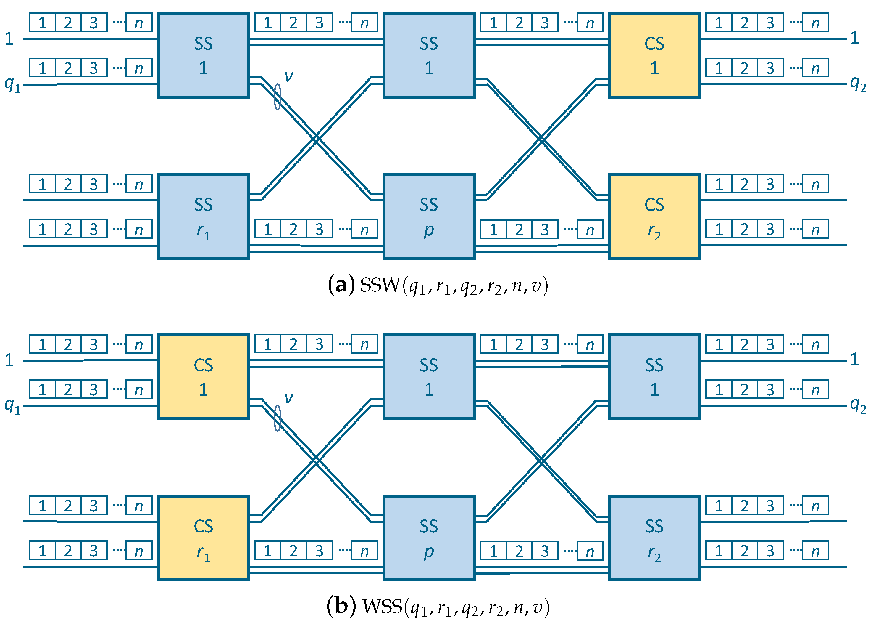
3. The Switching Fabric Architecture, Problem Statement, and Notation

The Architecture

In this article, we consider two types of three-stage switching networks, as shown in Figure 1. They consist of two types of switches: spectrum-converting switches (CSs) and space switches (SSs). The SS routes a connection from a set of FSUs on an input link to a set of FSUs with the same indexes on an output link. The CS can change the indexes of frequency slots, i.e., it can transfer connections from input links to output links by also changing the frequency slots occupied by connections.

In the first structure, shown in Figure 1a, the switching network consists of three stages, where the first two stages contain SSs, and the third stage is built of CSs. In the second structure, Figure 1b, the CSs are placed in the first stage, and the SSs form the second and third stages. Therefore, the first structure will be denoted by SSW (space–space–wavelength) and the second by WSS (wavelength–space–space). In both structures, the number of switches in the first stage is indicated by $r_1$, in the third stage it is indicated by $r_2$, and in the middle stage by p SSs. The switches in the first stage contain $q_1$ inputs with n FSUs per input, and switches in the third stage contain $q_2$ outputs and n FSUs per output. Due to SSs, the use of a different number of FSUs in the links does not make sense, because these switches only switch within the same FSUs. In addition, the switches of adjacent stages are generally connected by v links with n FSUs per link. The numbers $q_1$, $r_1$, $q_2$, $r_2$, n, and v uniquely define the structure of the switching network, and in the next part of the article, we will denote them as $\mathrm{SSW}(q_1,r_1,q_2,r_2,n,v)$ and $\mathrm{WSS}(q_1,r_1,q_2,r_2,n,v)$. In the case where $q_1=q_2=q$ and $r_1=r_2=r$, the switching network will be a symmetric network indicated by $\mathrm{SSW}(q,r,n,v)$ or $\mathrm{WSS}(q,r,n,v)$, depending on the structure.

Possible ways of implementing CSs are shown in Figure 2, assuming that the switch capacity is $q\times p$, n FSUs in each link. In all implementations, we assumed that in the most unfavorable case, each FSU must be converted to another FSU. The implementation shown in Figure 2a requires the largest number of converters. In CS version 1, each input link is fed to a Bandwidth-Variable Wavelength-Selective Switches (BV-WSS) with a capacity of $1\times np$, and each output of this switch is connected to one tunable spectrum converters (TSC). Then, the TSCs outputs in groups of n are fed to pasive combiners (PCs) with a capacity of $qn\times 1$, one PC for each output. The number of needed TSCs can be reduced by first converting the FSU and then redirecting the connection after conversion to the appropriate PC. This implementation is shown in Figure 2d. In this case, the capacity of a single BV-WSS and PCs is reduced. In turn, the implementations shown in Figure 2b,c use TSCs after directing the connection to the appropriate output. The implementation of SS is shown in Figure 3. In this case, there are no TSCs, and only BV-WSSs and PCs elements are used. The WSS and SSW networks look like inverses of each other. However, it should be emphasized that CSs in the WSS network are not the reverse of CSs in the SSW networks. The number of inputs and outputs of these switches varies and affects the number of BV-WSSs used. As we show in Section 5, depending on N and the selected parameters, $q_1$, $r_1$, $q_2$, and $r_2$, fewer of these elements may be in the WSS or SSW networks.

The switching network supports connections occupying a variable number of FSUs. The number of slots occupied by a connection (which can also include the guard band between connections) is denoted by m, the connection is called the m-slot connection, and the slots assigned to the connection must be adjacent. This value cannot exceed some maximum $m_{max}$ number of FSUs available on the input(output) link; that is, $1⩽m⩽m_{max}⩽n$. The new request appears at the input of ${\mathrm{I}}_i$ and must be connected to ${\mathrm{O}}_j$. This connection is denoted by $({\mathrm{I}}_i;{\mathrm{O}}_j;m)$, and since this is not important in our considerations, it does not refer to which FSUs are occupied. When a new $({\mathrm{I}}_i;{\mathrm{O}}_j;m)$ request appears at the input of ${\mathrm{I}}_i$, it is necessary to select m adjacent and free FSUs on the link leading from ${\mathrm{I}}_i$ to ${\mathrm{M}}_k$ in the middle stage. If the first-stage switches are SSs (SSW networks), the connection on this inter-stage link must be assigned the same FSUs as on the input link. Similarly, the same set of FSUs must be assigned in the link from ${\mathrm{M}}_k$ to ${\mathrm{O}}_j$. The spectrum conversion to the FSUs assigned to the connection on the output link occurs in ${\mathrm{O}}_j$, which is a spectrum-converting switch (CS). However, if the first-stage switches are CSs switches (WSS networks), in the inter-stage link from ${\mathrm{I}}_i$ to ${\mathrm{M}}_k$ the connection must occupy the same FSUs that are assigned in the output link because further in the following stages the conversion of the spectrum is no longer possible. In the article, we will determine in what case, i.e., with what number of switches in the middle stage, it is possible to set up any $({\mathrm{I}}_i;{\mathrm{O}}_j;m)$ using any ${\mathrm{M}}_k$ selection algorithm. The list of symbols used in the paper is listed in the Abbreviations on the end of the paper.

4. Strict-Sense Non-Blocking Conditions

In this section, we will derive the relationship between $q_1$, $q_2$, $m_{max}$, v, and p that ensures that any new m-slot connection can always be set up, provided that TSCs are available. These SNB conditions are derived and proved in the following theorems.

Theorem 1.

The $\mathrm{SSW}(q_1,r_1,q_2,r_2,n,v)$ switching network presented in Figure 1a is non-blocking in the strict sense for m-slot connections, $1⩽m⩽m_{max}⩽n$, if and only if:

$$\begin{array}{cc}p⩾p_{\mathrm{SNB}}^{\mathrm{SSW}}=\hfill & \underset{1⩽m⩽m_{max}}{max}\left\{⌊\frac{min\{\left(q_1-1\right)m;\left(r_2-1\right)q_{2}n\}}{v}⌋+⌊\frac{min\{q_{2}n-m;\left(r_1-1\right)q_{1}n\}}{v}⌋+1\right\}.\hfill \end{array}$$

(1)

Proof. 

We prove sufficiency by showing that we do not need more switches than those given by (1). Let us have a new connection request $({\mathrm{I}}_i;{\mathrm{O}}_j;m)$. In ${\mathrm{I}}_i$, this connection can be blocked by any other connection from other input links, using the same indexed FSUs. We have $q_1-1$ of such input links; for each link, there may be at most m 1-slot connections. However, the $(r_2-1)$ output switches (one switch is involved in the considered connection, so it is not included here) can accept at most $(r_2-1)q_{2}n$ connections; that is, the number of possible blocking connections is not greater than $min\{m(q_1-1);(r_2-1)q_{2}n\}$. One connection can block one link to the center-stage switches; therefore, the number of switches not accessible for the new connection is as follows:

$$p_1^{SSW}=⌊\frac{min\{\left(q_1-1\right)m;\left(r_2-1\right)q_{2}n\}}{v}⌋.$$

(2)

On the output side, connections in any FSUs can block the new request, since the output switch allows one to move connections to different slots. In ${\mathrm{O}}_j$, we may have at most $q_{2}n-m$ 1-slot blocking connections, but since they must be accepted in input switches, this number is not greater than $(r_1-1)q_{1}n$. Thus, the next set with

$$p_2^{SSW}=⌊\frac{min\{q_{2}n-m;\left(r_1-1\right)q_{1}n\}}{v}⌋$$

(3)

center-stage switches are unavailable for the new connection. In the worst-case scenario, these two sets of center-stage switches are disjoint, and one more switch is needed in the center stage, and we obtain Equation (1). □

Theorem 2.

The $\mathrm{WSS}(q_1,r_1,q_2,r_2,n,v)$ switching network presented in Figure 1b is non-blocking in the strict sense for m-channel connections, $1⩽m⩽m_{max}⩽n$, if and only if:

$$\begin{array}{cc}p⩾p_{\mathrm{SNB}}^{\mathrm{WSS}}=\hfill & \underset{1⩽m⩽m_{max}}{max}\left\{⌊\frac{min\{q_{1}n-m;\left(r_2-1\right)q_{2}n\}}{v}⌋+⌊\frac{min\{\left(q_2-1\right)m;\left(r_1-1\right)q_{1}n\}}{v}⌋+1\right\}\hfill \end{array}$$

(4)

Proof. 

The proof of this theorem is similar to the proof of Theorem 1. However, since we have wavelength switches in the first stage, the blocking connection can be established from any FSUs other than the one occupied by the new connection. The maximum number of potentially blocking connections is therefore not greater than $q_{1}n-m$, and this number is also limited by the number of available FSUs at the outputs, i.e., $\left(r_2-1\right)q_{2}n$. The number of center-stage switches unavailable for the new connection is, therefore, given by the following:

$$p_1^{WSS}=⌊\frac{min\{q_{1}n-m;\left(r_2-1\right)q_{2}n\}}{v}⌋$$

(5)

Similarly, the number of center-stage switches unavailable for a new connection due to other connections made to the ${\mathrm{O}}_j$ switch is determined as follows:

$$p_2^{WSS}=⌊\frac{min\{\left(q_2-1\right)m;\left(r_1-1\right)q_{1}n\}}{v}⌋$$

(6)

Since the new connection needs one more switch, the final number of switches needed in the center stage is given in (4). □

5. Cost Assessment and Comparison with Other Structures

In this section, we evaluate the costs of the proposed switching networks. The costs will be determined by the number of elements required for construction. First, we will analyze the number of switches in the center stage. However, this number alone does not clearly correspond to the cost of switching networks. Therefore, in the next parts of this section, we will take a closer look at assessing the number of elements required. We will consider TSCs first, which are the most expensive components, then BV-WSS and PCs, which in turn are the cheapest components with a negligible impact on the cost of the entire switching network. Importantly, we will compare these costs with the costs of other structures with similar parameters (SNB, number of inputs, and outputs) and show that by using the structures proposed in this work, we can reduce the number of required elements.

5.1. The Number of Switches

The number of center-stage switches is determined by Formulas (1) and (4) for the $\mathrm{SSW}(q_1,r_1,q_2,r_2,n,v)$ and $\mathrm{WSS}(q_1,r_1,q_2,r_2,n,v)$ networks, respectively. It can be seen from the formulas that the number of switches decreases as v increases. Therefore, we will analyze only switching networks with $v=1$; for $v>1$, the relationships between p and the remaining parameters of the switching networks are analogous. Figure 4 shows the dependence of the number of switches in the center stage p on m for switching networks with capacity $N=64$ and $n=20$. Different values of $q_1$ and $q_2$ were taken into account, but it should be remembered that the parameters $q_1$, $r_1$, $q_2$, and $r_2$ are related to each other by the relationship $N=q_1{r}_1=q_2{r}_2$. For constant values of $q_1$ or $q_2$, p increases with increasing m, but when $q_1=q_2$, p is constant and does not depend on m in the $\mathrm{SSW}(q_1,r_1,q_2,r_2,n,v)$ switching networks. At $m_{max}=n$, the SSW and WSS switching networks have the same value of p, and for $m_{max}<n$, the WSS networks require fewer switches in the center stage than the SSW networks. In both types of networks, for a given $m_{max}$, p decreases with decreasing $q_1$ and $q_2$, and reaches a minimum for $q_1=q_2=2$.

Let us look at some sample values. For a network with $N=64$ and $n=20$, the number of switches required in the middle stage is as follows. For $q_1=q_2=2$, p does not depend on $m_{max}$ and is 41 for the SSW network, but for the WSS network, p increases with $m_{max}$ from 5 for $m_{max}=2$ to 41 for $m_{max}=20$. When $q_1=q_2=8$, p increases with increasing $m_{max}$ for both the SSW and WSS networks. In the case of the SSW network, p changes from 173 for $m_{max}=2$ to 281 for $m_{max}=20$. In the WSS network, the change in p goes from 29 for $m_{max}=2$ also to 281 for $m_{max}=20$. When $q_1=q_2=32$, we have a change in p from 671 to 1241 in the SSW network and from 125 to 1241 in the WSS network, respectively. The basic conclusion that can be drawn from Figure 4, but also from similar calculations performed for other values of N, is that if $m_{max}<n$, we need fewer switches in the middle stage in the WSS networks, and when $m_{max}=n$, both structures require the same number of switches in the middle stage. Similar regularity can be observed for the cases where $q_1$ is different from $q_2$. For example, for $q_1=8$ and $q_2=32$ in the SSW networks, p increases from 653 for $m_{max}=2$ to 761 for $m_{max}=20$ in the SSW networks, and in the WSS networks, this change increases from 77 to 761.

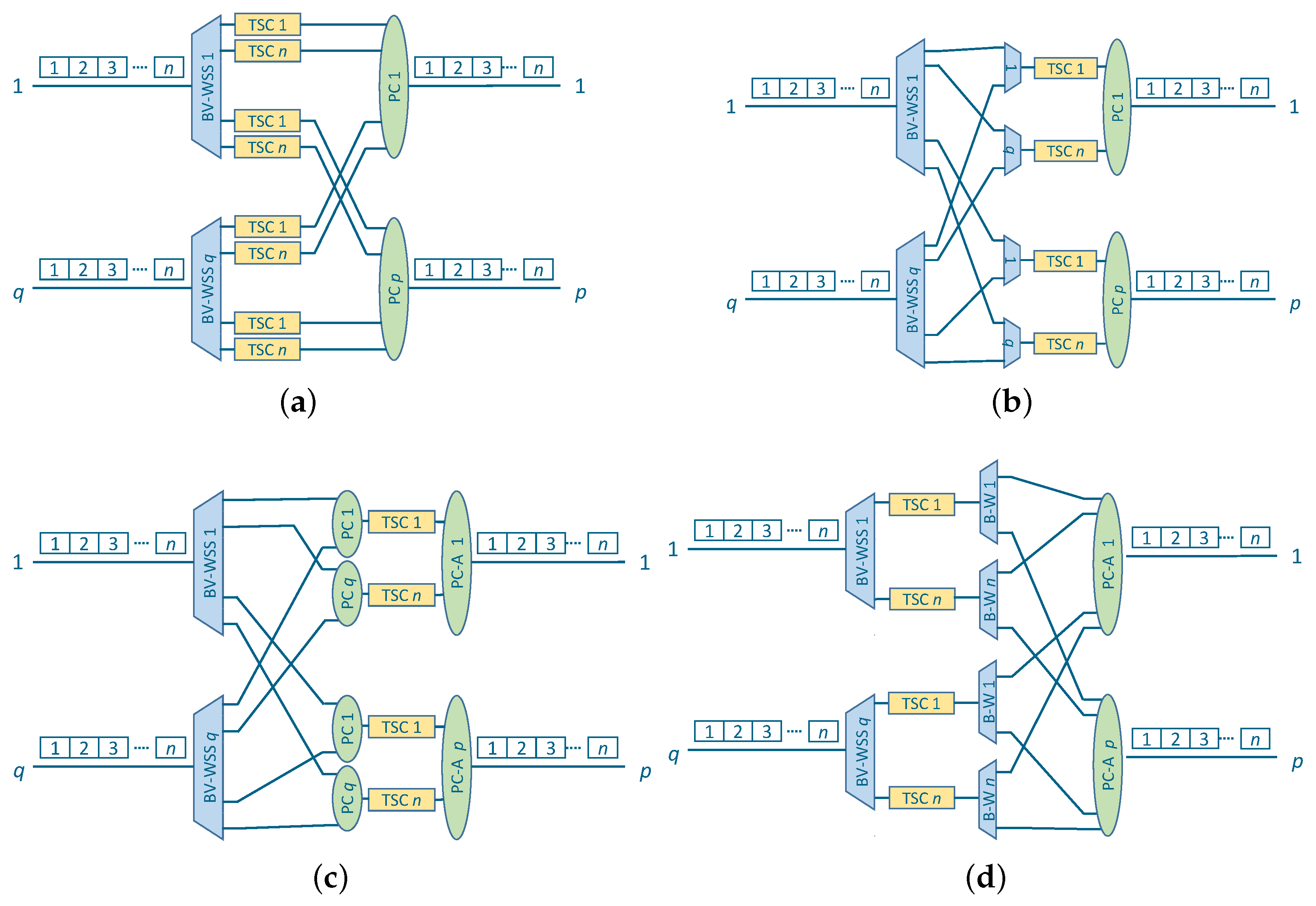
5.2. The Number of TSCs

Comparing network costs based on the number of switches in the center stage is not entirely reliable. A smaller number of center-stage switches generally results in a reduction in the number of inputs/outputs in the first-stage/third-stage switches, which in turn increases the number of switches in these stages, as well as the capacity of the center-stage switches. Therefore, it is more important to compare in terms of the number of elements needed to build switching networks. In this subsection, we will analyze the number of TSCs, which are the most expensive elements needed [60]. This number will be denoted by $C_{TSC}^{\mathrm{arch}}(ver.x)$, where arch takes the value SSW or WSS, and ver.x denotes the version of the CS implementation.

The number of TSCs in switching networks with different network structures and various versions of the CS implementation are determined by the following formulas:

$$\begin{array}{cc}\hfill C_{\mathrm{TSC}}^{\mathrm{SSW}}\left(\mathrm{ver.1}\right)& =npv{q}_2{r}_2,\hfill \end{array}$$

(7)

$$\begin{array}{cc}\hfill C_{\mathrm{TSC}}^{\mathrm{SSW}}\left(\mathrm{ver.2}\right)& =n{q}_2{r}_2,\hfill \end{array}$$

(8)

$$\begin{array}{cc}\hfill C_{\mathrm{TSC}}^{\mathrm{SSW}}\left(\mathrm{ver.3}\right)& =n{q}_2{r}_2,\hfill \end{array}$$

(9)

$$\begin{array}{cc}\hfill C_{\mathrm{TSC}}^{\mathrm{SSW}}\left(\mathrm{ver.4}\right)& =npv{r}_2,\hfill \end{array}$$

(10)

$$\begin{array}{cc}\hfill C_{\mathrm{TSC}}^{\mathrm{WSS}}\left(\mathrm{ver.1}\right)& =npv{q}_1{r}_1,\hfill \end{array}$$

(11)

$$\begin{array}{cc}\hfill C_{\mathrm{TSC}}^{\mathrm{WSS}}\left(\mathrm{ver.2}\right)& =npv{r}_1,\hfill \end{array}$$

(12)

$$\begin{array}{cc}\hfill C_{\mathrm{TSC}}^{\mathrm{WSS}}\left(\mathrm{ver.3}\right)& =npv{r}_1,\hfill \end{array}$$

(13)

$$\begin{array}{cc}\hfill C_{\mathrm{TSC}}^{\mathrm{WSS}}\left(\mathrm{ver.4}\right)& =n{q}_1{r}_1.\hfill \end{array}$$

(14)

Analyzing these formulas, it can be noticed that $pv>q_1$ and $pv>q_2$, i.e., in the SSW networks, the least numbers of TSCs are for ver.2 and ver.3, and in the WSS networks—for ver.4. If the switching network has N inputs and N outputs, then since $N=q_2{r}_2=q_1{r}_1$, the number of TSCs is given by

$$C_{\mathrm{TSC}}=nN,$$

(15)

and it does not depend on p and v. This is also the smallest required number of TSCs, which ensures the conversion of all FSUs in the most unfavorable case. It does not depend on the size of $q_i$ and $r_i$, so it does not matter how the inputs/outputs are divided between the switches of the external stages.

Table 1. The number of required TSCs in various switching networks with $N=64$ and different values of n; $m_{max}=n$.

n	SSW	WSS	WSW	SWS1	SWS2
20	1280	1280	2560	25,400	26,240
40	2560	2560	5120	101,600	103,680
60	3840	3840	7680	228,600	232,320
80	5120	5120	10,240	406,400	412,160
100	6400	6400	12,800	635,000	643,200
120	7680	7680	15,360	914,400	925,440
140	8960	8960	17,920	1,244,600	1,258,880
160	10,240	10,240	20,480	1,625,600	1,643,520
320	20,480	20,480	40,960	6,502,080	6,563,840

shows sample costs of the SSW and WSS networks with different capacities, and the WSW and SWS networks for comparison. This table summarizes the required number of TSCs for various values of n in networks with $N=64$. It can be seen that WSW networks always require at least twice as many TSCs as SSW or WSS networks. Much more TSCs are needed in SWS networks, which is due to the number of switches in the middle stage, where these TSCs are found. If connections must occupy a minimum of 2 FSUs (the data channel and guard band), the number of converters required can be reduced by half.

5.3. The Number of BV-WSS and PCs

Since the $N\times N$ switching network with the smallest number of TSCs can be constructed assuming different values of $q_1$, $r_1$, $q_2$, and $r_2$, we will now analyze at what values of these parameters it will contain the fewest BV-WSSs (they are more expensive than PCs). Since the number of BV-WSSs and PCs in CSs varies depending on how they are implemented, the formulas for the number of these elements vary depending on the version of the implementation. In the case of BV-WSSs, the number of these elements is determined by the formulas:

$$\begin{array}{cc}\hfill C_{\mathrm{BV-WSS}}^{\mathrm{SSW}}\left(\mathrm{ver.1}\right)& =q_1{r}_1+pv{r}_1+pv{r}_2,\hfill \end{array}$$

(16)

$$\begin{array}{cc}\hfill C_{\mathrm{BV-WSS}}^{\mathrm{SSW}}\left(\mathrm{ver.2}\right)& =q_1{r}_1+pv{r}_1+pv{r}_2+n{q}_2{r}_2,\hfill \end{array}$$

(17)

$$\begin{array}{cc}\hfill C_{\mathrm{BV-WSS}}^{\mathrm{SSW}}\left(\mathrm{ver.3}\right)& =q_1{r}_1+pv{r}_1+pv{r}_2,\hfill \end{array}$$

(18)

$$\begin{array}{cc}\hfill C_{\mathrm{BV-WSS}}^{\mathrm{SSW}}\left(\mathrm{ver.4}\right)& =q_1{r}_1+pv{r}_1+pv{r}_2+npv{r}_2,\hfill \end{array}$$

(19)

$$\begin{array}{cc}\hfill C_{\mathrm{BV-WSS}}^{\mathrm{WSS}}\left(\mathrm{ver.1}\right)& =q_1{r}_1+pv{r}_1+pv{r}_2,\hfill \end{array}$$

(20)

$$\begin{array}{cc}\hfill C_{\mathrm{BV-WSS}}^{\mathrm{WSS}}\left(\mathrm{ver.2}\right)& =q_1{r}_1+npv{r}_2+pv{r}_1+pv{r}_2,\hfill \end{array}$$

(21)

$$\begin{array}{cc}\hfill C_{\mathrm{BV-WSS}}^{\mathrm{WSS}}\left(\mathrm{ver.3}\right)& =q_1{r}_1+pv{r}_1+pv{r}_2,\hfill \end{array}$$

(22)

$$\begin{array}{cc}\hfill C_{\mathrm{BV-WSS}}^{\mathrm{WSS}}\left(\mathrm{ver.4}\right)& =q_1{r}_1+n{q}_1{r}_1+pv{r}_1+pv{r}_2.\hfill \end{array}$$

(23)

For PCs, the relevant formulas are as follows:

$$\begin{array}{cc}\hfill C_{\mathrm{PC}}^{\mathrm{SSW}}\left(\mathrm{ver.1}\right)& =q_2{r}_2+pv{r}_1+pv{r}_2,\hfill \end{array}$$

(24)

$$\begin{array}{cc}\hfill C_{\mathrm{PC}}^{\mathrm{SSW}}\left(\mathrm{ver.2}\right)& =q_2{r}_2+pv{r}_1+pv{r}_2,\hfill \end{array}$$

(25)

$$\begin{array}{cc}\hfill C_{\mathrm{PC}}^{\mathrm{SSW}}\left(\mathrm{ver.3}\right)& =q_2{r}_2+n{q}_2{r}_2+pv{r}_1+pv{r}_2,\hfill \end{array}$$

(26)

$$\begin{array}{cc}\hfill C_{\mathrm{PC}}^{\mathrm{SSW}}\left(\mathrm{ver.4}\right)& =q_2{r}_2+pv{r}_1+pv{r}_2,\hfill \end{array}$$

(27)

$$\begin{array}{cc}\hfill C_{\mathrm{PC}}^{\mathrm{WSS}}\left(\mathrm{ver.1}\right)& =q_2{r}_2+pv{r}_2+pv{r}_1,\hfill \end{array}$$

(28)

$$\begin{array}{cc}\hfill C_{\mathrm{PC}}^{\mathrm{WSS}}\left(\mathrm{ver.2}\right)& =q_2{r}_2+pv{r}_2+pv{r}_1,\hfill \end{array}$$

(29)

$$\begin{array}{cc}\hfill C_{\mathrm{PC}}^{\mathrm{WSS}}\left(\mathrm{ver.3}\right)& =q_2{r}_2+pv{r}_2+pv{r}_1+npv{r}_1,\hfill \end{array}$$

(30)

$$\begin{array}{cc}\hfill C_{\mathrm{PC}}^{\mathrm{WSS}}\left(\mathrm{ver.4}\right)& =q_2{r}_2+pv{r}_2+pv{r}_1,\hfill \end{array}$$

(31)

Since the costs of costs BV-WSSs are several dozen times higher than the costs of PCs, we will limit the analysis to the networks with the lowest number of these first elements [60]. When determining switching networks with the smallest number of BV-WSSs, we will only take into account the networks in which the number of TSCs is minimal; that is, versions 2 and 3 for SSW networks and version 4 for WSS networks. In the analysis, we also limited the number of parallel inter-stage links v to values no greater than $min\{q_1/2,q_2/2\}$. Comparing Formulas (17) and (18), it can be seen that $C_{\mathrm{BV-WSS}}^{\mathrm{SSW}}\left(\mathrm{ver.2}\right)>C_{\mathrm{BV-WSS}}^{\mathrm{SSW}}\left(\mathrm{ver.3}\right)$, because in Formula (17), there is an additional term, $n{q}_2{r}_2$, which is always greater than zero. Therefore, further analyses and graphs are limited to WSS networks with the version 3 implementation of CSs. At the same time, for Formulas (25) and (26), we have the opposite relationship; that is, $C_{\mathrm{PC}}^{\mathrm{SSW}}\left(\mathrm{ver.2}\right)<C_{\mathrm{PC}}^{\mathrm{SSW}}\left(\mathrm{ver.3}\right)$.

The first conclusion is quite obvious; that is, the number of BV-WSSs increases as $m_{max}$ increases. The only exception is switching networks with $q_1=q_2=2$, where p is constant and does not depend on $m_{max}$. In turn, for a given $m_{max}$, this number varies depending on v.

Table 2. The number of required BV-WSSs in $\mathrm{WSS}(32,2,32,2,20,v)$ switching networks versus $m_{max}$ for different values of v; the minimum values in each column are marked in bold red.

m=	1	2	3	4	5	6	7	8	9	10	11	12	13	14	15	16	17	18	19	20
v = 1	1596	1844	2092	2340	2588	2836	3084	3332	3580	3828	4076	4324	4572	4820	5068	5316	5564	5812	6060	6308
v = 2	1592	1848	2088	2344	2584	2840	3080	3336	3576	3832	4072	4328	4568	4824	5064	5320	5560	5816	6056	6312
v = 3	1596	1836	2100	2340	2580	2844	3084	3324	3588	3828	4068	4332	4572	4812	5076	5316	5556	5820	6060	6300
v = 4	1584	1840	2096	2352	2576	2832	3088	3344	3568	3824	4080	4336	4560	4816	5072	5328	5552	5808	6064	6320
v = 5	1604	1844	2084	2324	2604	2844	3084	3324	3564	3844	4084	4324	4564	4804	5084	5324	5564	5804	6044	6324
v = 6	1608	1848	2088	2328	2568	2856	3096	3336	3576	3816	4056	4344	4584	4824	5064	5304	5544	5832	6072	6312
v = 7	1596	1820	2100	2324	2604	2828	3108	3332	3556	3836	4060	4340	4564	4844	5068	5292	5572	5796	6076	6300
v = 8	1568	1824	2080	2336	2592	2848	3104	3360	3552	3808	4064	4320	4576	4832	5088	5344	5536	5792	6048	6304
v =9	1596	1812	2100	2316	2604	2820	3108	3324	3612	3828	4044	4332	4548	4836	5052	5340	5556	5844	6060	6276
v = 10	1624	1864	2104	2344	2584	2824	3064	3304	3544	3864	4104	4344	4584	4824	5064	5304	5544	5784	6024	6344
v = 11	1564	1828	2092	2356	2620	2796	3060	3324	3588	3852	4116	4292	4556	4820	5084	5348	5524	5788	6052	6316
v = 12	1584	1872	2064	2352	2544	2832	3120	3312	3600	3792	4080	4368	4560	4848	5040	5328	5520	5808	6096	6288
v = 13	1604	1812	2124	2332	2540	2852	3060	3372	3580	3788	4100	4308	4620	4828	5036	5348	5556	5764	6076	6284
v = 14	1624	1848	2072	2296	2632	2856	3080	3304	3528	3864	4088	4312	4536	4872	5096	5320	5544	5768	6104	6328
v = 15	1644	1884	2124	2364	2604	2844	3084	3324	3564	3804	4044	4284	4524	4764	5124	5364	5604	5844	6084	6324
v = 16	1536	1792	2048	2304	2560	2816	3072	3328	3584	3840	4096	4352	4608	4864	5120	5376	5504	5760	6016	6272

shows the dependence of $C_{\mathrm{BV-WSS}}^{\mathrm{WSS}}\left(\mathrm{ver.4}\right)$ given in (23) on $m_{max}$ for different values of v and the switching networks $\mathrm{WSS}(32,2,32,2,20,v)$. It can be seen that the minimum number of BV-WSSs is achieved for different values of v. For example, for $m_{max}=4$, the minimum number of BV-WSSs equal to 2296 is achieved at $v=14$; for $m_{max}=6$, the minimum equal to 2796 is reached at $v=11$; and for $m_{max}=8$, the minimum occurs at $V=10$ and is 3304. A similar pattern occurs for SSW networks.

Table 3. The number of required BV-WSSs in $64\times 64$ WSS and SSW networks for different values of $q_1$, $q_2$, and $m_{max}$.

WSS
	${\mathit{q}}_{\mathbf{1}}$ = 32			${\mathit{q}}_{\mathbf{1}}$ = 16			${\mathit{q}}_{\mathbf{1}}$ = 8
m=	4	6	8	4	6	8	4	6	8
$q_2$ = 32	2296	2796	3304	2436	2982	3558	2874	3624	4374
$q_2$ = 16	2436	2982	3558	2296	2744	3272	2412	2928	3468
$q_2$ = 8	2874	3624	4374	2412	2928	3468	2256	2688	3120
$q_2$ = 4	3810	5034	6258	2804	3524	4244	2328	2808	3288
$q_2$ = 2	5730	7906	10082	3684	4836	5988	2664	3304	3944
SSW
	${\mathit{q}}_{\mathbf{1}}$ = 32			${\mathit{q}}_{\mathbf{1}}$ = 16			${\mathit{q}}_{\mathbf{1}}$ = 8
m=	4	6	8	4	6	8	4	6	8
$q_2$ = 32	3072	3320	3568	4222	4390	4582	6714	6824	6934
$q_2$ = 16	2692	3046	3424	3072	3256	3528	4204	4348	4492
$q_2$ = 8	2874	3464	4054	2668	2992	3340	3024	3200	3376
$q_2$ = 4	3682	4762	5842	2804	3364	3924	2584	2872	3160
$q_2$ = 2	5538	7578	9618	3556	4564	5572	2664	3144	3624

compares the number of BV-WSSs in the WSS and SSW switching networks with $N=64$ for different values of $q_1$, $q_2$, and $m_{max}$. It can be seen that the number of these elements changes and reaches a minimum for different values of $q_1$ and $q_2$. For example, in WSS networks, for $q_1=32$, the number of BV-WSSs increases as $q_2$ decreases, but for $q_1=16$, the minimum is reached at $q_2=16$ and for $q_1=8$ at $q_2=$8. In turn, in SSW networks, for $q_1=32$, the number of these elements reaches the minimum at $q_2=16$; for $q_1=16$—at $q_2=8$; and for $q_1=8$—at $q_2=4$.

Figure 5 shows the dependence of the minimum number of BV-WSSs in the WSS and SSW networks, depending on $m_{max}$. It shows that for $m_{max}=10$ this number is the same in both networks and is 2688, for $m_{max}<10$ the WSS networks contain fewer elements, and for $m_{max}>$ 10 fewer items are in the SSW networks. For WSS networks, the minimum number of BV-WSSs occur when $q_1=q_2=2$ and $v=1$ regardless of $m_{max}$. In SSW networks, this minimum also occurs with the same value of these parameters, but from $m_{max}>6$. For $3\le m_{max}\le 6$, the minimum is reached when $q_1=4$, $q_2=2$ and $v=1$, and for $m_{max}=2$, the least BV-WSSs are achieved in a network with $q_1=8$, $q_2=2$, and $v=1$.

5.4. Cost Assessment Summary

From the cost analyses, it can be concluded that the proposed WSS and SSW networks require the smallest number of the most expensive elements, which are wavelength converters. Alternative WSW or SWS networks with the same characteristics and capacity require at least twice as many of these elements. A smaller number of converters will only be needed in blocking networks, where not all optical paths will require bandwidth conversion. We also showed that the network structure choice is significantly influenced by the network capacity and the maximum number of frequency slots assigned to the optical path. Depending on N and $m_{max}$, the number of converters in the WSS and SSW networks will be the same, but the number of BV-WSSs needed will depend on the division of inputs ($q_1$) and outputs ($q_2$) between switches of the first ($r_1$) and third ($r_2$) stages and the selected number of inter-stage links v, respectively. Determining the optimal network structure is simple and requires checking all possible parameter values, where N must be a multiple of q and r. For example, for $N=64$, it suffices to calculate (using Formulas (7)–(31)) the number of elements for $q_1$, and $q_2$ belonging to the set $\{2,4,8,16,32\}$, and v is within the limits of 1 to $min\{q_1,q_2\}/2$.

6. Conclusions and Future Work

In this article, we propose two versions of the three-stage optical switching networks: $\mathrm{WSS}(q_1,r_1,q_2,r_2,n,v)$ and $\mathrm{SSW}(q_1,r_1,q_2,r_2,n,v)$. These networks contain bandwidth-converting switches only in the first or third stages. For these networks, we derive strict-sense non-blocking conditions. As expected, placing switches with conversion in only one stage reduces the number of converters required by half compared to WSW networks. SWS networks also contain bandwidth-converting switches in a single stage, but their number is much larger for non-blocking operations, which affects the number of converters. We show that the SSW and WSS networks require the fewest TSCs, which is equal to the number of FSUs in the input and output links. Fewer of these components will not support connection sets where each requires spectrum conversion. For switching networks with a minimum number of TSCs, we show that WSS networks require a smaller number of switches in the middle section, while in the case of BV-WSSs, their number is smaller in WSS networks only up to certain values, $m_{max}$, then SSW networks are more favorable. It should be noted that this limit may vary depending on N and n. The SNB conditions derived in the article are accurate analytical results and ensure that the blocking probability is reduced to zero. Therefore, they do not require additional verification by means of simulation and the use of specialized simulation software, such as, for example, in the work of [45,46].

Further reduction in network costs will be possible using routing algorithms with the functional decomposition of middle-stage switches into groups that serve connections within certain limited ranges of values, m, as considered in the WSW networks [56]. However, it is expected that this will reduce the number of center-stage switches and, therefore, BV-WSSs elements.

References

1. CISCO. 2023 Global Netwroking Trends Survey Results; Technical Report; CISCO: San Jose, CA, USA, 2023. [Google Scholar]
2. CISCO. Cisco: Annual Internet Report (2018–2023); Technical Report; CISCO: San Jose, CA, USA, 2020. [Google Scholar] [CrossRef]
3. Jinno, M.; Takara, H.; Kozicki, B.; Tsukishima, Y.; Sone, Y.; Matsuoka, S. Spectrum-Efficient and Scalable Elastic Optical Path Network: Architecture, Benefits, and Enabling Technologies. IEEE Commun. Mag. 2009, 47, 66–73. [Google Scholar] [CrossRef]
4. Gerstel, O.; Jinno, M.; Lord, A.; Yoo, S.J.B. Elastic Optical Networking: A New Dawn for the Optical Layer? IEEE Commun. Mag. 2012, 50, S12–S20. [Google Scholar] [CrossRef]
5. Tomkos, I.; Azodolmolky, S.; Sole-Pareta, J.; Careglio, D.; Palkopoulou, E. A Tutorial on the Flexible Optical Networking Paradigm: State of the Art, Trends, and Research Challenges. Proc. IEEE 2014, 102, 1317–1337. [Google Scholar] [CrossRef]
6. ITU-T. ITU-T Recommendation G.694.1. Spectral Grids for WDM Applications: DWDM Frequency Grid; International Telecommunication Union–Telecommunication Standardization Sector (ITU-T): Geneva, Switzerland, 2012. [Google Scholar]
7. Chatterjee, B.C.; Sarma, N.; Oki, E. Routing and Spectrum Allocation in Elastic Optical Networks: A Tutorial. IEEE Commun. Surv. Tutor. 2015, 17, 1776–1800. [Google Scholar] [CrossRef]
8. Chadha, D. Optical WDM Networks: From Static to Elastic Networks; Wiley IEEE Press: Hoboken, NJ, USA, 2019; pp. 1–373. [Google Scholar] [CrossRef]
9. Chatterjee, B.C.; Oki, E. Elastic Optical Networks: Fundamentals, Design, Control, and Management; CRC Press: Boca Raton, FL, USA, 2020. [Google Scholar] [CrossRef]
10. Filer, M.; Gaudette, J.; Ghobadi, M.; Mahajan, R.; Issenhuth, T.; Klinkers, B.; Cox, J. Elastic optical networking in the Microsoft cloud [invited]. J. Opt. Commun. Netw. 2016, 8, A45–A54. [Google Scholar] [CrossRef]
11. Aibin, M.; Walkowiak, K. Analysis of inter-data center elastic optical network. In Proceedings of the 2017 19th International Conference on Transparent Optical Networks (ICTON), Girona, Spain, 2–6 July 2017; pp. 1–4. [Google Scholar] [CrossRef]
12. Amri, F.S.; Huang, Z.; Liu, K.; Pan, J. Energy-Aware Inter-Data Center VM Migration Over Elastic Optical Networks. In Proceedings of the GLOBECOM 2023—2023 IEEE Global Communications Conference, Kuala Lumpur, Malaysia, 4–8 December 2023; pp. 5421–5426. [Google Scholar] [CrossRef]
13. Nakada, K.; Takeshita, H.; Kuno, Y.; Matsuno, Y.; Urashima, I.; Shimomura, Y.; Jinno, M. Single Multicore-Fiber Bidirectional Spatial Channel Network Based on Spatial Cross-Connect and Multicore EDFA Efficiently Accommodating Asymmetric Traffic. In Proceedings of the 2023 Optical Fiber Communications Conference and Exhibition (OFC), San Diego, CA, USA, 5–9 March 2023; pp. 1–3. [Google Scholar] [CrossRef]
14. Winzer, P.J.; Neilson, D.T.; Chraplyvy, A.R. Fiber-optic transmission and networking: The previous 20 and the next 20 years [Invited]. Opt. Express 2018, 26, 24190–24239. [Google Scholar] [CrossRef] [PubMed]
15. Alshowkan, M.; Lukens, J.M.; Lu, H.H.; Kirby, B.T.; Williams, B.P.; Grice, W.P.; Peters, N.A. Broadband polarization-entangled source for C + L-band flex-grid quantum networks. Opt. Lett. 2022, 47, 6480–6483. [Google Scholar] [CrossRef] [PubMed]
16. Lin, J.; Chang, T.; Zhai, Z.; Bose, S.K.; Shen, G. Wavelength Selective Switch-Based Clos Network: Blocking Theory and Performance Analyses. J. Light. Technol. 2022, 40, 5842–5853. [Google Scholar] [CrossRef]
17. Mehrvar, H.; Li, S.; Bernier, E. Dimensioning networks of ROADM cluster nodes. J. Opt. Commun. Netw. 2023, 15, C166–C178. [Google Scholar] [CrossRef]
18. Cheng, Z.; Ye, T.; Zhu, Y.; Hu, W. A Three-Phase Modularization Approach of OXC for Large-Scale ROADM. J. Light. Technol. 2023, 41, 7318–7327. [Google Scholar] [CrossRef]
19. Mano, T.; Inoue, T.; Mizutani, K.; Akashi, O. Redesigning the Nonblocking Clos Network to Increase Its Capacity. IEEE Trans. Netw. Serv. Manag. 2023, 20, 2558–2574. [Google Scholar] [CrossRef]
20. Svaluto Moreolo, M.; Spadaro, S.; Calabretta, N. Optical Switching Systems and Flex-Grid Technologies. In Handbook of Radio and Optical Networks Convergence; Kawanishi, T., Ed.; Springer Nature Singapore: Singapore, 2023; pp. 1–37. [Google Scholar] [CrossRef]
21. Yao, Y.; Ye, T.; Deng, N. Nonblocking conditions for flex-grid OXC–Clos Networks. In Proceedings of the IEEE INFOCOM 2024—IEEE Conference on Computer Communications, Vancouver, BC, Canada, 20–23 May 2024; pp. 1–10. [Google Scholar]
22. Huang, Z.; Yang, S.; Zheng, Z.; Pan, X.; Li, H.; Yang, H. Highly Compact Twin 1 × 35 Wavelength Selective Switch. J. Light. Technol. 2023, 41, 233–239. [Google Scholar] [CrossRef]
23. Patsamanis, G.; Ketzaki, D.; Chatzitheocharis, D.; Vyrsokinos, K. Optical Design of a Wavelength Selective Switch Utilizing a Waveguide Frontend with Beamsteering Capability. Photonics 2024, 11, 381. [Google Scholar] [CrossRef]
24. Ma, Y.; Stewart, L.; Armstrong, J.; Clarke, I.G.; Baxter, G. Recent Progress of Wavelength Selective Switch. J. Light. Technol. 2021, 39, 896–903. [Google Scholar] [CrossRef]
25. Chatterjee, B.C.; Ba, S.; Oki, E. Fragmentation Problems and Management Approaches in Elastic Optical Networks: A Survey. IEEE Commun. Surv. Tutor. 2018, 20, 183–210. [Google Scholar] [CrossRef]
26. Zhang, P.; Li, J.; Guo, B.; He, Y.; Chen, Z.; Wu, H. Comparison of Node Architectures for Elastic Optical Networks with Waveband Conversion. China Commun. 2013, 10, 77–87. [Google Scholar]
27. Kabaciński, W.; Michalski, M.; Rajewski, R. Strict-Sense Nonblocking W-S-W Node Architectures for Elastic Optical Networks. J. Light. Tech. 2016, 34, 3155–3162. [Google Scholar] [CrossRef]
28. Danilewicz, G.; Kabaciński, W.; Rajewski, R. Strict-sense nonblocking space-wavelength-space switching fabrics for elastic optical network nodes. J. Opt. Commun. Netw. 2016, 8, 745–756. [Google Scholar] [CrossRef]
29. Clos, C. A study of non-blocking switching networks. Bell Syst. Tech. J. 1953, 32, 406–424. [Google Scholar] [CrossRef]
30. Kabaciński, W.; Al-Tameemie, A.; Rajewski, R. Necessary and Sufficient Conditions for the Rearrangeability of WSW1 Switching Fabrics. IEEE Access 2019, 7, 18622–18633. [Google Scholar] [CrossRef]
31. Lin, B.C. Rearrangeable W-S-W elastic optical networks generated by graph approaches: Erratum. IEEE/OSA J. Opt. Commun. Netw. 2019, 11, 282–284. [Google Scholar] [CrossRef]
32. Lin, B. New upper bound for a rearrangeable non-blocking WSW architecture. IET Commun. 2019, 13, 3425–3433. [Google Scholar] [CrossRef]
33. Danilewicz, G. Asymmetrical Space-Conversion-Space SCS1 Strict-Sense and Wide-Sense Nonblocking Switching Fabrics for Continuous Multislot Connections. IEEE Access 2019, 7, 107058–107072. [Google Scholar] [CrossRef]
34. Danilewicz, G. Supplement to “Asymmetrical Space-Conversion Space SCS1 Strict-Sense and Wide-Sense Nonblocking Switching Fabrics for Continuous Multislot Connections”—The SCS2 Switching Fabrics Case. IEEE Access 2019, 7, 167577–167583. [Google Scholar] [CrossRef]
35. Lin, B.C. Rearrangeable and Repackable S-W-S Elastic Optical Networks for Connections with Limited Bandwidths. Appl. Sci. 2020, 10, 1251. [Google Scholar] [CrossRef]
36. López, V.; Velasco, L. Elastic Optical Networks. Architectures, Technologies, and Control; Springer International Publishing: Cham, Switzerland, 2016. [Google Scholar]
37. Khodashenas, P.; Rivas-Moscoso, J.; Shariati, B.; Marom, D.; Klonidis, D.; Tomkos, I. Investigation of Spectrum Granularity for Performance Optimization of Flexible Nyquist-WDM-Based Optical Networks. J. Light. Technol. 2015, 33, 4767–4774. [Google Scholar] [CrossRef]
38. Tomkos, I.; Khodashenas, P.S.; Rivas-Moscoso, J.M.; Klonidis, D. Switching and Routing for Spatially and Spectrally Flexible Elastic Optical Networking (IEEE HPSR 2015 Tutorial). In Proceedings of the High Performance Switching and Routing (HPSR), Budapest, Hungary, 1–4 July 2015. [Google Scholar]
39. Tomkos, I.; Miyamoto, Y.; Wellbrock, G.; Winzer, P.J. Spatially and Spectrally Flexible Elastic Optical Networking (Guest Editiorial). IEEE Commun. Mag. 2015, 53, 20–22. [Google Scholar] [CrossRef]
40. Song, M.; Pincemin, E.; Josten, A.; Baeuerle, B.; Hillerkuss, D.; Leuthold, J.; Rudnick, R.; Marom, D.M.; Ben Ezra, S.; Ferran, J.F.; et al. Flexible Optical Cross-Connects for High Bit Rate Elastic Photonic Transport Networks [Invited]. J. Opt. Commun. Netw. 2016, 8, 126–140. [Google Scholar] [CrossRef]
41. Marom, D.M.; Colbourne, P.D.; Errico, A.D.; Fontaine, N.K.; Proietti, R.; Zong, L.; Rivas-moscoso, J.M.; Tomkos, I. Survey of Photonic Switching Architectures and Technologies in Support of Spatially and Spectrally Flexible Optical Networking [Invited]. J. Opt. Commun. Netw. 2017, 9, 1–26. [Google Scholar] [CrossRef]
42. Liu, H.; Sang, L.; Chen, Y. A multicast contention resolution scheme based on shared spectrum converter for elastic optical switching node. Opt.-Int. J. Light Electron Opt. 2017, 144, 316–323. [Google Scholar] [CrossRef]
43. Xie, D.; Wang, D.; Zhang, M.; Liu, Z.; You, Q.; Yang, Q.; Yu, S. LCoS-Based Wavelength-Selective Switch for Future Finer-Grid Elastic Optical Networks Capable of All-Optical Wavelength Conversion. IEEE Photonics J. 2017, 9, 7101212. [Google Scholar] [CrossRef]
44. Stasiak, M.; Sobieraj, M.; Zwierzykowski, P. Modeling of Multi-Service Switching Networks with Multicast Connections. IEEE Access 2022, 10, 5359–5377. [Google Scholar] [CrossRef]
45. Glabowski, M.; Sobieraj, M.; Stasiak, M. Analytical Model of a Single Link of Elastic Optical Networks. IEEE Access 2022, 10, 90200–90212. [Google Scholar] [CrossRef]
46. Gła̧bowski, M.; Ivanov, H.; Leitgeb, E.; Sobieraj, M.; Stasiak, M. Simulation studies of elastic optical networks based on 3-stage Clos switching fabric. Opt. Switch. Netw. 2020, 36, 100555. [Google Scholar] [CrossRef]
47. Sobieraj, M.; Zwierzykowski, P.; Leitgeb, E. Simulation Studies of Elastic Optical Networks Nodes with Multicast Connections. Hum.-Centric Comput. Inf. Sci. 2022, 12, 5. [Google Scholar] [CrossRef]
48. Beneš, V.E. Mathematical Theory of Connecting Networks and Telephone Traffic; Academic Press: New York, USA, 1965. [Google Scholar]
49. Pattavina, A. Switching Theory; John Wiley & Sons, Inc.: Chichester, England, 1998. [Google Scholar]
50. Hwang, F. The Mathematical Theory of Nonblocking Switching Networks, 2nd ed.; World Scientific Publishing Co., Inc.: Hackensack, NJ, USA; London, UK, 2004; Volume 15. [Google Scholar]
51. Kabaciński, W. Nonblocking Electronic and Photonic Switching Fabrics; Springer: New York, NY, USA, 2005. [Google Scholar]
52. Kabaciński, W.; Michalski, M.; Abdulsahib, M. The Strict-Sense Nonblocking Elastic Optical Switch. In Proceedings of the IEEE 25th International Conference on High Performance Switching and Routing (HPSR), Budapest, Hungary, 1–4 July 2015. [Google Scholar]
53. Kabaciński, W.; Michalski, M.; Abdulsahib, M. Wide-Sense Nonblocking Elastic Optical Switch. Opt. Switch. Netw. 2017, 25, 71–79. [Google Scholar] [CrossRef]
54. Kabaciński, W.; Abdulsahib, M.; Michalski, M. Wide-sense nonblocking W-S-W node architectures for elastic optical networks. IEICE Trans. Commun. 2019, E102-B, 978–991. [Google Scholar] [CrossRef]
55. Kabacinski, W.; Al-Tameemie, A.; Rajewski, R. Rearrangeability of Wavelength-Space-Wavelength Switching Fabric Architecture for Elastic Optical Switches. IEEE Access 2019, 7, 64993–65006. [Google Scholar] [CrossRef]
56. Kabaciński, W.; Abdulsahib, M. Wide-sense nonblocking converting-space-converting switching node architecture under XsVarSWITCH control algorithm. IEEE/ACM Trans. Netw. 2020, 28, 1550–1561. [Google Scholar] [CrossRef]
57. Abuelela, E.; Żal, M.; Kabaciński, W. Simultaneous Connections Routing in Wavelength–Space–Wavelength Elastic Optical Switches. Sensors 2023, 23, 3615. [Google Scholar] [CrossRef]
58. Abdulsahib, M.; Kabaciński, W. The Strict-Sense Nonblocking S-S-W Elastic Optical Switching Fabric; Technical Report TR-KK-33/2/2019/A; Poznan University of Technology: Poznań, Poland, 2019. [Google Scholar]
59. Abdulsahib, M.; Kabaciński, W. Comparisons between W-S-W, S-W-S, and S-S-W Switching Fabric Architectures in Terms of Required Switching Elements; Technical Report TR-KK-35/4/2019/A; Poznan University of Technology: Poznań, Poland, 2019. [Google Scholar]
60. De Groote, M.; Manousakis, K.; Kokkinos, P.; Colle, D.; Pickavet, M.; Christodoulopoulos, K.; Varvarigos, E.; Demeester, P. Cost comparison of different translucent optical network architectures. In Proceedings of the 2010 9th Conference of Telecommunication, Media and Internet, CTTE 2010, Ghent, Belgium, 7–9 June 2010; pp. 1–8. [Google Scholar] [CrossRef]
Figure 1. The switching fabric architectures: (a) space–space–wavelength, and (b) wavelength–space–space.
Electronics 13 02544 g001
Figure 2. Implementations of CS: (a) version 1, (b) version 2, (c) version 3, and (d) version 4.
Electronics 13 02544 g002
Figure 3. Implementations of SS.
Electronics 13 02544 g003
Figure 4. The number of center-stage switches p versus m max in SSW ( q 1 , r 1 , q 2 , r 2 , n , v ) and WSS ( q 1 , r 1 , q 2 , r 2 , n , v ) switching networks with N = 64 , v = 1 , and n = 20 .
Electronics 13 02544 g004
Figure 5. The minimum number of BV-WSSs versus m max in SSW and WSS switching networks with N = 64 and n = 20 .
Electronics 13 02544 g005