
Malware Detection and Classification System Based on CNN-BiLSTM


Abstract
1. Introduction
2. Related Works
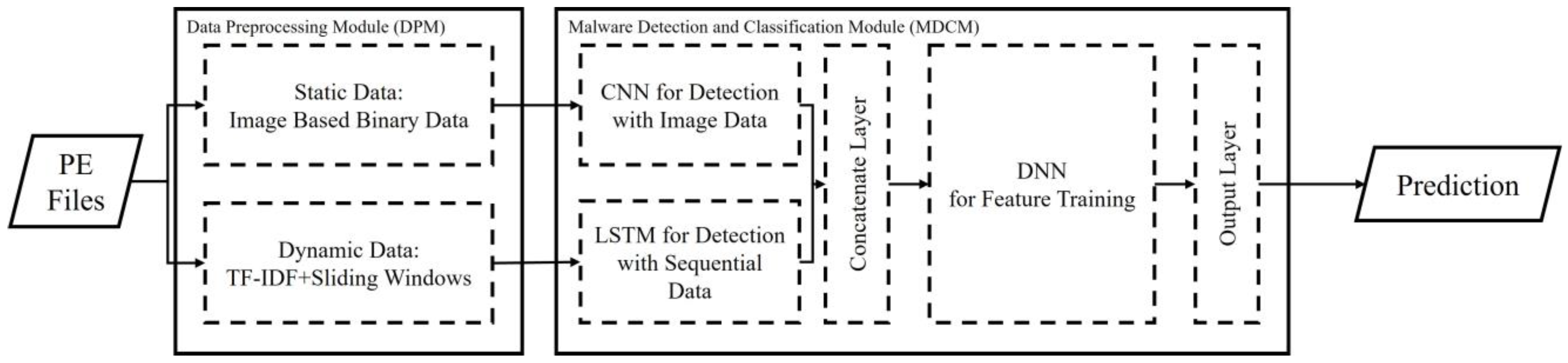
3. Proposed System
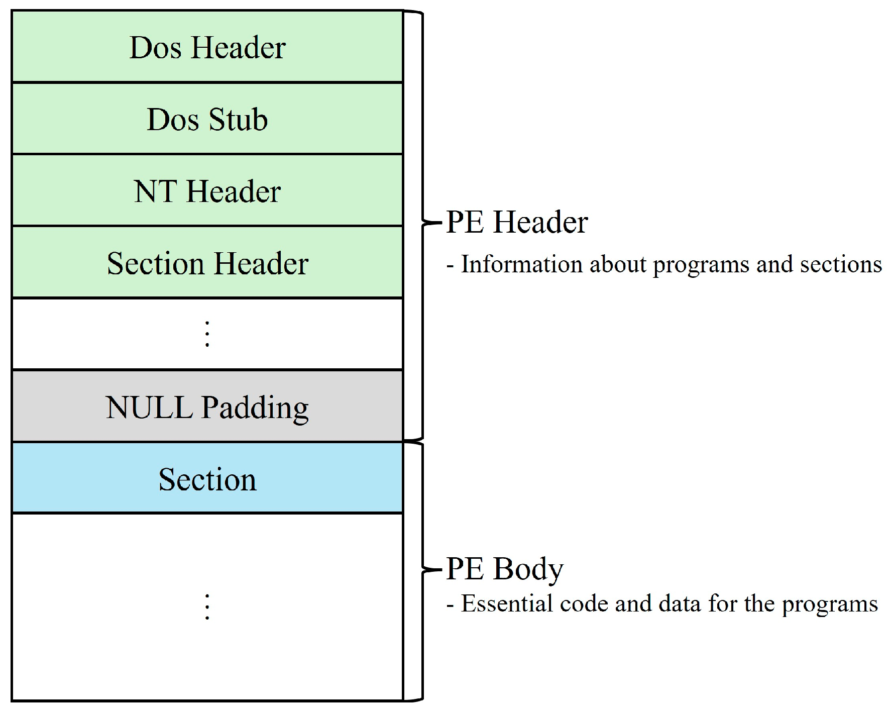
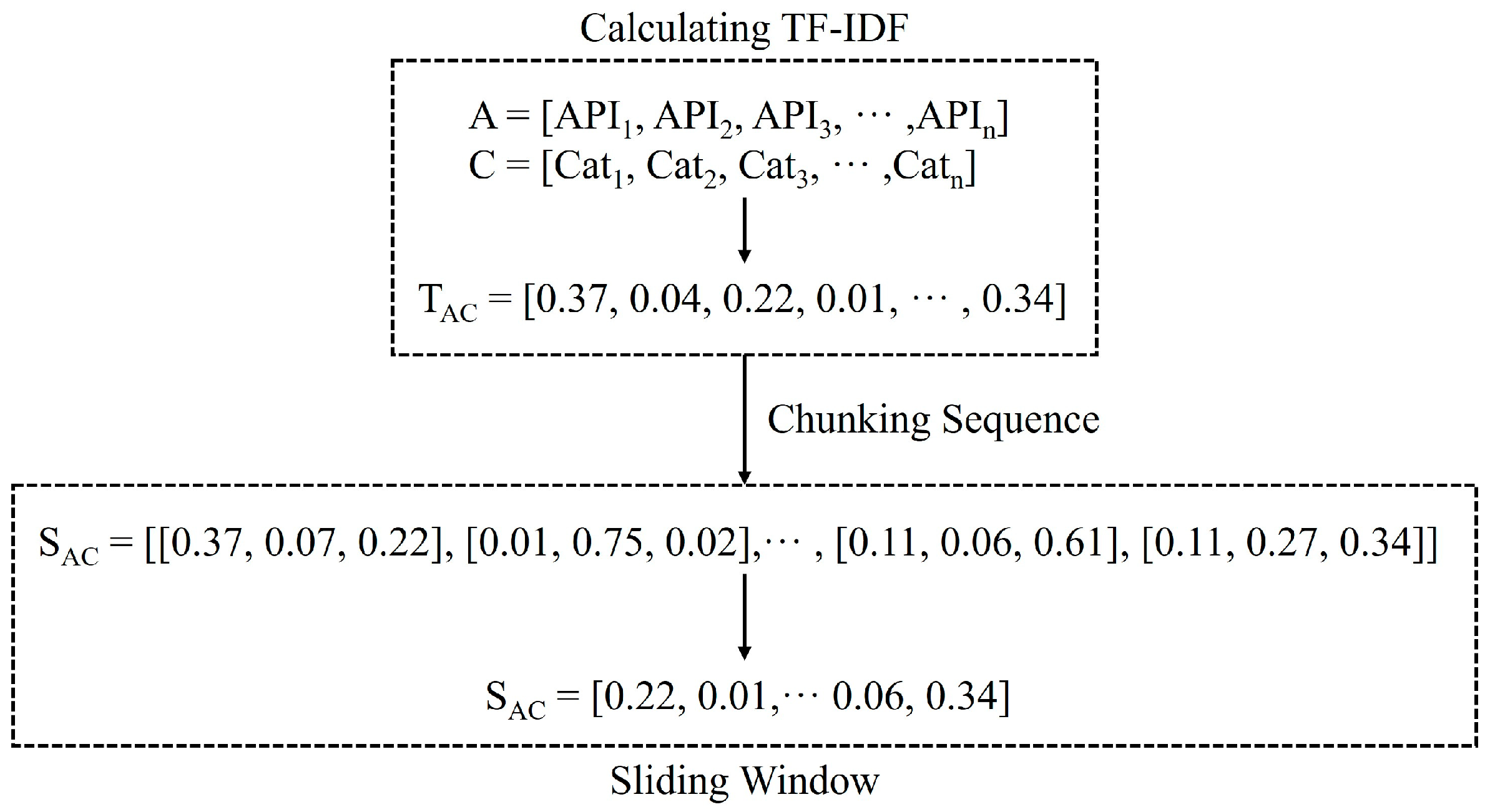
3.1. Data Preprocessing Module (DPM)
| Algorithm 1: Proposed TF-IDF and sliding window calculation algorithm | |
| Input: API call sequences ; Categories ; Target length for transformation | |
| Output: Preprocessed data | |
| /*Calculating TF-IDF*/ | |
| 1 | Calculating as TFIDF |
| 2 | Calculating as TFIDF |
| 3 | |
| /*Chunking Sequence*/ | |
| 4 | ← Dividing by |
| 5 | Type Casting to integer |
| 6 | Initialize |
| 7 | for ← 0 to length of and increment steps are do |
| 8 | if = (length of ) then |
| 9 | ← |
| 10 | break |
| 11 | end |
| 12 | Extract size of elements from and add to |
| 13 | |
| 14 | end |
| 15 | for ← to length of and increment steps are do |
| 16 | Extract size of elements from and add to |
| 17 | end |
| /*Sliding Window*/ | |
| 18 | ← Calculating the average of each window in |
| 19 | ← Calculate the final values in using |
| 20 | return |
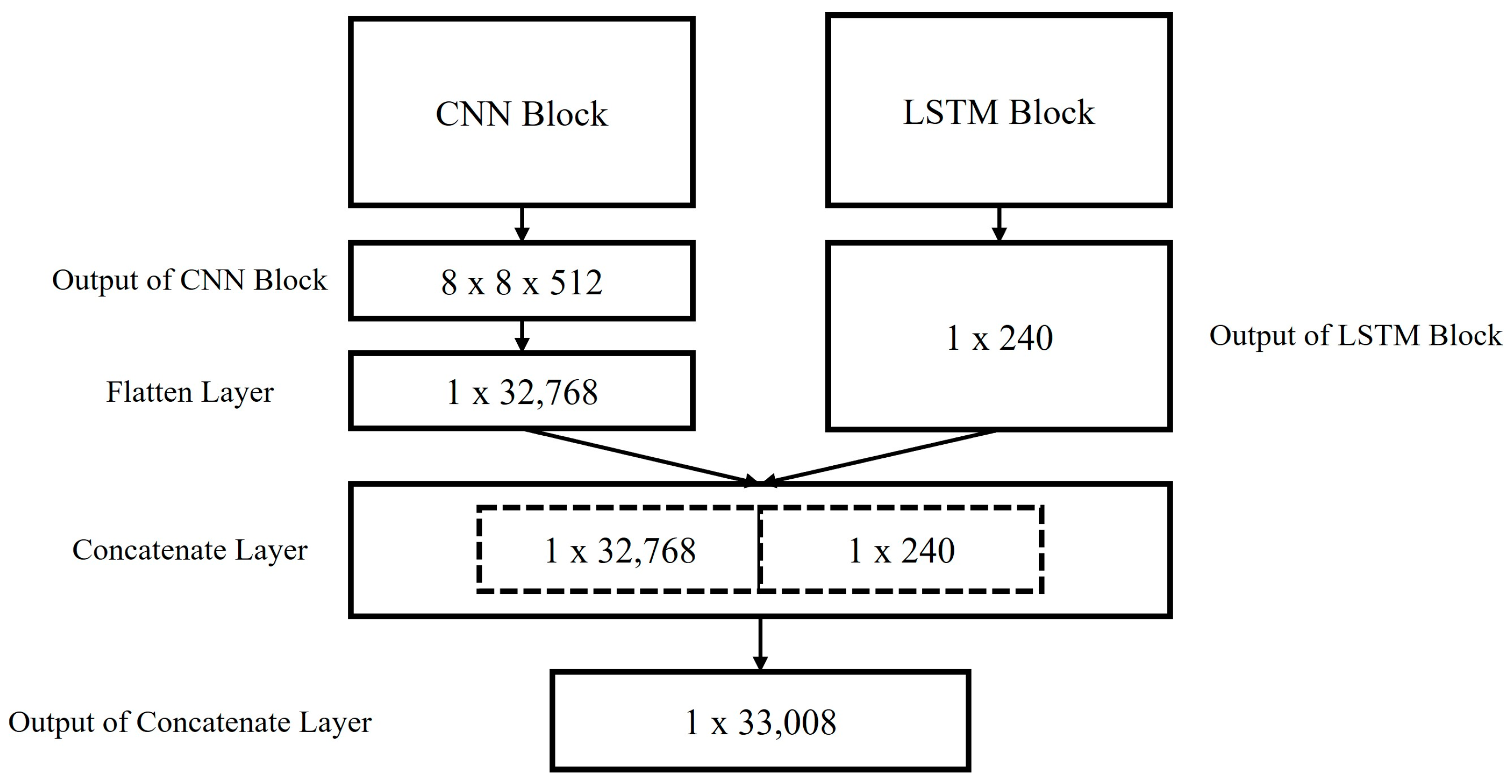
3.2. Malware Detection and Classification Module (MDCM)
3.2.1. Convolutional Neural Network (CNN)
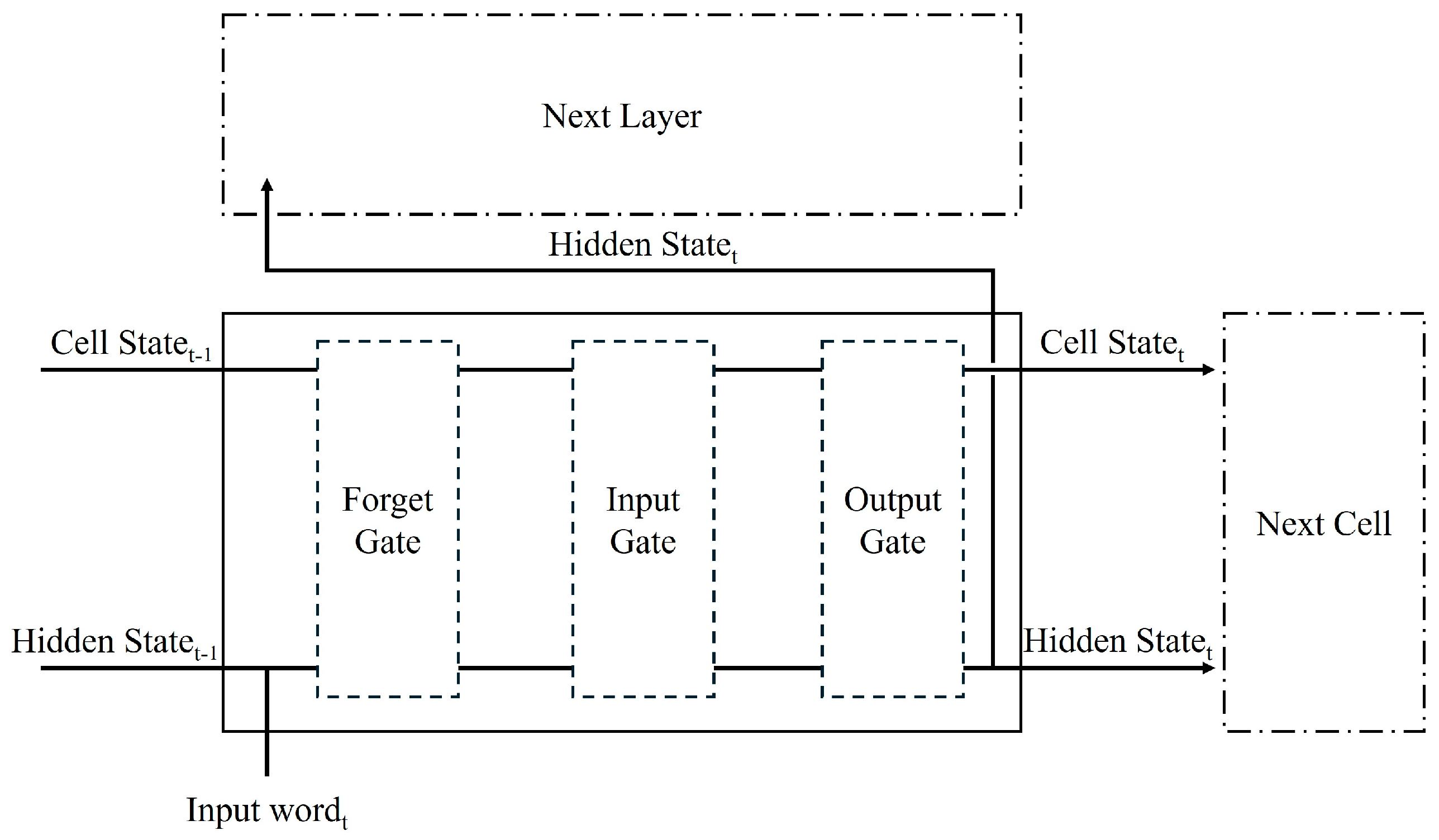
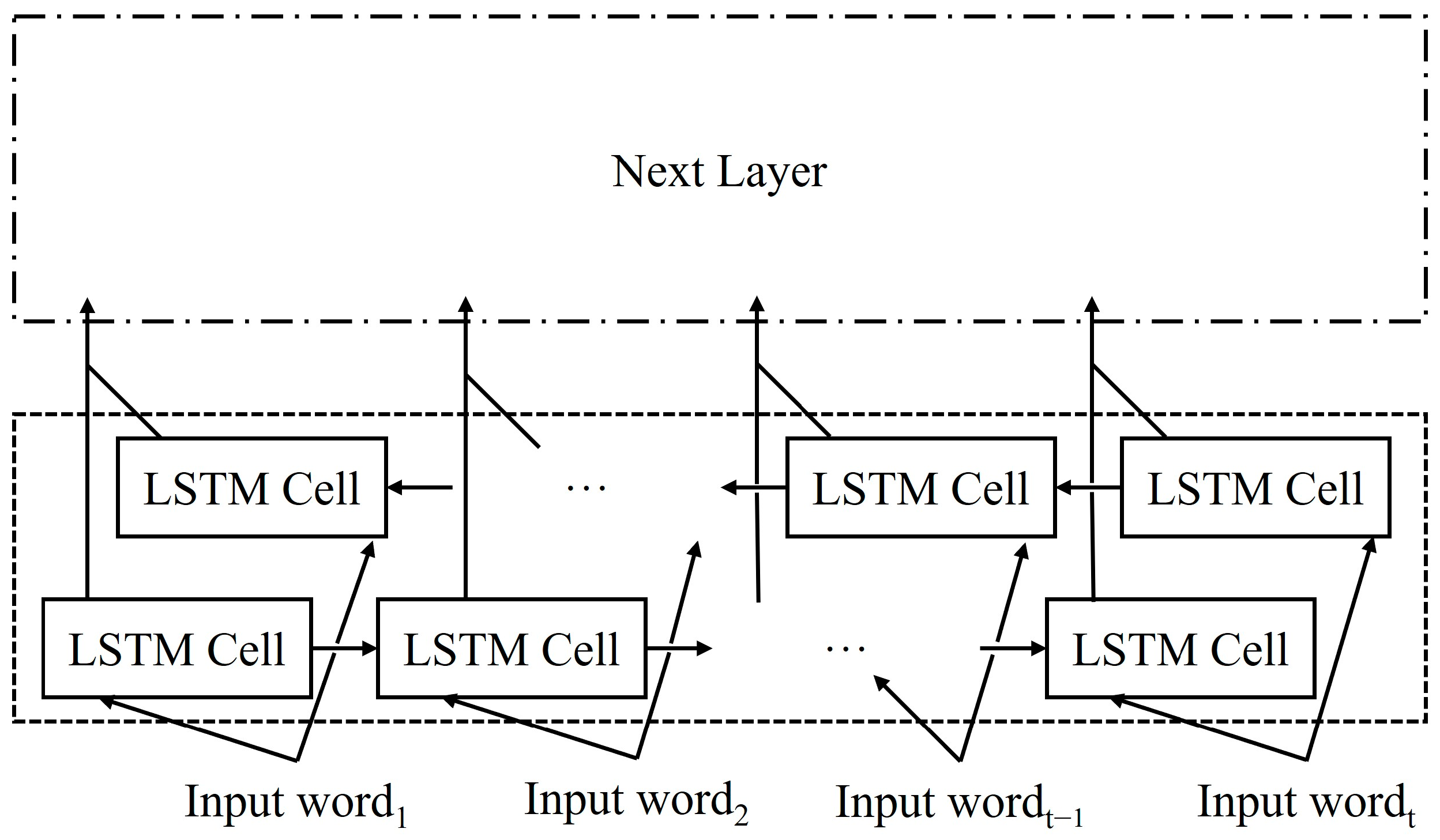
3.2.2. Long Short-Term Memory (LSTM)
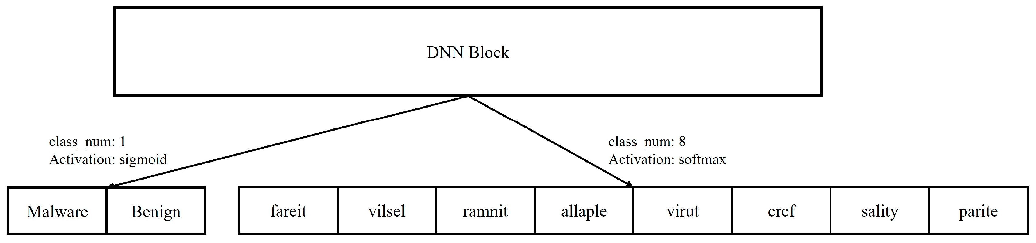
3.2.3. Deep Neural Network (DNN)
4. Performance Evaluation
4.1. Experimental Environments
4.2. Experimental Dataset
4.3. Experimental Methods
4.4. Experimental Results
5. Conclusions
Author Contributions
Funding
Data Availability Statement
Conflicts of Interest
References
- O’Kane, P.; Sezer, S.; McLaughlin, K. Obfuscation: The Hidden Malware. IEEE Secur. Priv. 2011, 9, 41–47. [Google Scholar] [CrossRef]
- Azeez, N.A.; Odufuwa, O.E.; Misra, S.; Oluranti, J.; Damaševičius, R. Windows PE Malware Detection Using Ensemble Learning. Informatics 2021, 8, 10. [Google Scholar] [CrossRef]
- O’Shea, K.; Nash, R. An Introduction to Convolutional Neural Networks. arXiv 2015, arXiv:1511.08458. [Google Scholar]
- Vasan, D.; Alazab, M.; Wassan, S.; Safaei, B.; Zheng, Q. Image-Based malware classification using ensemble of CNN architectures (IMCEC). Comput. Secur. 2020, 92, 101748. [Google Scholar] [CrossRef]
- Kumar, S.; Panda, K. SDIF-CNN: Stacking deep image features using fine-tuned convolution neural network models for real-world malware detection and classification. Appl. Soft Comput. 2023, 146, 110676. [Google Scholar] [CrossRef]
- Naeem, H.; Dong, S.; Falana, O.J.; Ullah, F. Development of a deep stacked ensemble with process based volatile memory forensics for platform independent malware detection and classification. Expert Syst. Appl. 2023, 223, 119952. [Google Scholar] [CrossRef]
- Yadava, P.; Menonb, N.; Ravic, V.; Vishvanathand, S.; Phame, D.T. A two-stage deep learning framework for image-based android malware detection and variant classification. Comput. Intell. 2022, 38, 1748–1771. [Google Scholar] [CrossRef]
- Gómez, A.; Muñoz, A. Deep Learning-Based Attack Detection and Classification in Android Devices. Electronics 2023, 12, 3253. [Google Scholar] [CrossRef]
- Hochreiter, S.; Schmidhuber, J. Long short-term memory. Neural Comput. 1997, 9, 1735–1780. [Google Scholar] [CrossRef]
- Kim, H.; Kim, M. Malware Detection System Based on Static-Dynamic preprocessing Techniques Combined in an Ensemble Model. In Proceedings of the 15th International Conference on Computer Science and Its Applications, Nha Trang, Vietnam, 18–20 December 2023. not published yet. [Google Scholar]
- Han, X.; Zhang, Z.; Ding, N.; Gu, Y.; Liu, X.; Huo, Y.; Qiu, J.; Yao, Y.; Zhang, A.; Zhang, L.; et al. Pre-trained models: Past, present and future. AI Open 2021, 2, 225–250. [Google Scholar] [CrossRef]
- PE Format. Available online: https://learn.microsoft.com/en-us/windows/win32/debug/pe-format (accessed on 10 April 2024).
- Nataraj, L.; Karthikeyan, S.; Jacob, G.; Manjunath, B.S. Malware images: Visualization and automatic classification. In Proceedings of the 8th International Symposium on Visualization for Cyber Security, Pittsburgh, PA, USA, 20 June 2011; pp. 1–7. [Google Scholar]
- Cuckoo Sandbox—Automated Malware Analysis. Available online: https://cuckoo.readthedocs.io/en/latest/ (accessed on 10 April 2024).
- Kim, M.; Kim, H. A Dynamic Analysis Data Preprocessing Technique for Malicious Code Detection with TF-IDF and Sliding Windows. Electronics 2024, 13, 963. [Google Scholar] [CrossRef]
- Graves, A.; Schmidhuber, J. Framewise Phoneme Classification with Bidirectional LSTM Networks. In Proceedings of the International Joint Conference on Neural Networks, Montreal, Canada, 31 July–4 August 2005; pp. 2047–2052. [Google Scholar]
- PE Malware Machine Learning Dataset. Available online: https://practicalsecurityanalytics.com/pe-malware-machine-learning-dataset/ (accessed on 10 April 2024).
- VirusTotal. Available online: https://www.virustotal.com/gui/home/upload (accessed on 7 June 2024).
- GitHub Repository. Available online: https://github.com/haesookimDev/MalDetectIntegrantedSystem/tree/main/Data (accessed on 10 April 2024).


| Layer | Parameters | Values | Output |
|---|---|---|---|
| Input Layer | 256, 256, 1 | 256, 256, 1 | |
| Convolutional Layer_1 | filter | 32 | 256, 256, 32 |
| kernel_size | 3, 3 | ||
| strides | 1 | ||
| activation | Rectified Linear Unit (ReLU) | ||
| Max Pooling Layer_1 | pool_size | 2, 2 | 128, 128, 32 |
| Convolutional Layer_2 | filter | 64 | 128, 128, 64 |
| kernel_size | 3, 3 | ||
| strides | 1 | ||
| activation | ReLU | ||
| Max Pooling Layer_2 | pool_size | 2, 2 | 64, 64, 64 |
| Convolutional Layer_3 | filter | 128 | 64, 64, 128 |
| kernel_size | 3, 3 | ||
| strides | 1 | ||
| activation | ReLU | ||
| Max Pooling Layer_3 | pool_size | 2, 2 | 32, 32, 128 |
| Convolutional Layer_4 | filter | 256 | 32, 32, 256 |
| kernel_size | 3, 3 | ||
| strides | 1 | ||
| activation | ReLU | ||
| Max Pooling Layer_4 | pool_size | 2, 2 | 16, 16, 256 |
| Convolutional Layer_3 | filter | 512 | 16, 16, 512 |
| kernel_size | 3, 3 | ||
| strides | 1 | ||
| activation | ReLU | ||
| Max Pooling Layer_3 | pool_size | 2, 2 | 8, 8, 512 |
| Dropout Layer | rate | 0.2 | 8, 8, 512 |
| Flatten Layer | 32,768 |
| Layer | Parameters | Values | Output | |
|---|---|---|---|---|
| Input Layer | 1, Target length | 1, Target length | ||
| Bidirectional Layer 1 | LSTM | units | 120 | 1, 240 |
| return sequences | True | |||
| Bidirectional Layer 2 | LSTM | units | 120 | 240 |
| Layer | Parameters | Values | Output |
|---|---|---|---|
| Concatenate Layer | 32,768 | 33,008 | |
| 240 | |||
| Batch Normalization Layer 1 | 33,008 | ||
| Dense Layer 1 | units | 512 | 512 |
| activation | ReLU | ||
| Batch Normalization Layer 2 | 512 | ||
| Dense Layer 2 | units | 256 | 256 |
| activation | ReLU | ||
| Batch Normalization Layer 3 | 256 | ||
| Dense Layer 3 | units | 128 | 128 |
| activation | ReLU | ||
| Dense Layer 4 | units | class_num | class_num |
| activation | sigmoid or softmax |
| Hardware | Specification |
|---|---|
| CPU | Intel Xeon(R) Silver 4215R 3.20 GHz |
| RAM | 256 GB DDR4 |
| GPU | RTX QUADRO A6000 |
| VRAM | 48 GB GDDR6 |
| Library | Version |
|---|---|
| Python | 3.7.13 |
| TensorFlow | 2.7.0 |
| Scikit-learn | 1.0.2 |
| NumPy | 1.21.6 |
| Pandas | 1.3.5 |
| Type | Count |
|---|---|
| Trojan.fareit | 3095 |
| Trojan.vilsel | 2308 |
| Virus.ramnit | 2113 |
| Worm.allaple | 1524 |
| Virus.virut | 1478 |
| Trojan.crcf | 1248 |
| Virus.sality | 1047 |
| Virus.parite | 983 |
| Methods | Lengths | Acc (%) | Classify-Acc (%) | Recall (%) | Precision (%) | F1 score |
|---|---|---|---|---|---|---|
| Detect–Classify | 400 | 99.27 | 94.93 | 99.34 | 99.42 | 0.9938 |
| Classify | 99.39 | 95.21 | 99.6 | 99.74 | 0.9967 | |
| Detect–Classify | 800 | 99.17 | 95.08 | 99.45 | 99.13 | 0.9929 |
| Classify | 99.39 | 94.87 | 99.74 | 99.6 | 0.9967 | |
| Detect–Classify | 1200 | 99.44 | 94.97 | 99.6 | 99.45 | 0.9953 |
| Classify | 99.39 | 94.49 | 99.46 | 99.89 | 0.9967 | |
| Detect–Classify | 2000 | 99.34 | 95.4 | 99.67 | 99.2 | 0.9944 |
| Classify | 99.18 | 95.28 | 99.78 | 99.34 | 0.9956 |
| Methods | Lengths | Max Total Time (s) | Min Total Time (s) | Avg Total Time (s) |
|---|---|---|---|---|
| Detect–Classify | 400 | 0.1515 | 0.1121 | 0.1311 |
| Classify | 0.083 | 0.058 | 0.0697 | |
| Detect–Classify | 800 | 0.1548 | 0.1154 | 0.1351 |
| Classify | 0.0824 | 0.0597 | 0.071 | |
| Detect–Classify | 1200 | 0.1611 | 0.1157 | 0.1336 |
| Classify | 0.0803 | 0.0585 | 0.0663 | |
| Detect–Classify | 2000 | 0.1581 | 0.1152 | 0.1399 |
| Classify | 0.0839 | 0.0577 | 0.0668 |
| Reference | Methods | Dataset | Detect Acc (%) | Classification Acc (%) | F1 score | Time (s) |
|---|---|---|---|---|---|---|
| Azeez et al. [2] | PCA + MLP, CNN | Benign: 5012 Malware: 14,599 | 1.0 | N/A | 1.0 | N/A |
| Vasan et al. [4] | Image + VGG16, ResNet-50 PCA + SVM | Malware: 9339 | N/A | 99.5 | N/A | 1.18 |
| Kumar et al. [5] | Image + VGG16 VGG19, ResNet-50, InceptionV3 | Malware: 9339 | N/A | 98.55 | 0.99 | 0.471 |
| Naeem et al. [6] | Image, LBP, GLCM + CNN | Benign: 608 Malware: 3686 | 99.1 | N/A | 0.99 | 1.82 |
| Yadava et al. [7] | Image + EfficientNetB0, SVM, Random Forest | Benign: 4826 Malware: 2486 | 100 | 89 | 1.0 | N/A |
| Gomez et al. [8] | Static Feature + Machine Learning | Malware: 16,890 | 99.01 | N/A | 0.986 | N/A |
| This Paper | Image + CNN API call sequence + LSTM | Benign: 9756 Malware: 13,796 | 99.44 | 95.4 | 0.9967 | 0.0663 |
Disclaimer/Publisher’s Note: The statements, opinions and data contained in all publications are solely those of the individual author(s) and contributor(s) and not of MDPI and/or the editor(s). MDPI and/or the editor(s) disclaim responsibility for any injury to people or property resulting from any ideas, methods, instructions or products referred to in the content. |
© 2024 by the authors. Licensee MDPI, Basel, Switzerland. This article is an open access article distributed under the terms and conditions of the Creative Commons Attribution (CC BY) license (https://creativecommons.org/licenses/by/4.0/).
Share and Cite
Kim, H.; Kim, M. Malware Detection and Classification System Based on CNN-BiLSTM. Electronics 2024, 13, 2539. https://doi.org/10.3390/electronics13132539
Kim H, Kim M. Malware Detection and Classification System Based on CNN-BiLSTM. Electronics. 2024; 13(13):2539. https://doi.org/10.3390/electronics13132539
Chicago/Turabian StyleKim, Haesoo, and Mihui Kim. 2024. "Malware Detection and Classification System Based on CNN-BiLSTM" Electronics 13, no. 13: 2539. https://doi.org/10.3390/electronics13132539
APA StyleKim, H., & Kim, M. (2024). Malware Detection and Classification System Based on CNN-BiLSTM. Electronics, 13(13), 2539. https://doi.org/10.3390/electronics13132539