Motion Equations and Attitude Control in the Vertical Flight of a VTOL Bi-Rotor UAV: Part 2

Abstract

This paper gathers the dynamical modeling of an unmanned aircraft and the design and simulation of the control system, allowing it to perform a Vertical Take-Off (VTOL) maneuver, a fixed-wing (FW) flight and a transition between the two configurations using two tilting rotors (Bi-Tilt). These Unmanned Aerial Vehicles (UAVs) operating in this configuration are categorized as Hybrid UAVs, for their capability of having a dual flight envelope: flying like a multi-rotor and navigating like a traditional fixed-wing aircraft, allowing the drone to perform complex missions where these two flight configurations are essential. This work exhibits the Bi-Rotor non-linear dynamics, valid for both flight configurations, the design of the control algorithm for stability and navigation, and a simulation of a complete flight mission.

1. Introduction

Nowadays, significant advancements in engineering disciplines such as automation systems, flight control, and the aerospace sector have propelled the rapid expansion of Unmanned Aerial Vehicles (UAVs). These UAVs have emerged as a prominent research interest and are applicable in both military and civilian domains. Civil applications span agricultural services, marine operations, disaster response, infrastructure inspection, environmental monitoring, and delivery services. In the military field, UAVs are primarily deployed in high-risk missions, where human involvement is impractical.

To enhance the versatility and efficiency of these applications, there is a growing demand for UAVs capable of dual flight modes. These hybrid UAVs combine the benefits of traditional fixed-wing aircraft and rotorcraft, facilitating Vertical Take-Off and Landing (VTOL) and enabling high-speed aerial surveillance across extensive areas. This hybrid capability makes UAVs highly valuable for a diverse range of operations.

According to Ref. [1], hybrid UAVs can be categorized into two main types: Convertiplanes and Tail-Sitters. First of all, the Convertiplanes category regroups those aerial vehicles that take off, cruise, hover and land with the aircraft reference line remaining horizontal. With respect to this class, there exist several vehicles implementing the idea, such as FireFLY6 [2] and TURAC [3], and also projects researching in this direction [4,5]. Second, a Tail-Sitter is an aircraft that takes off and lands vertically on its tail, and the whole aircraft tilts forward using differential thrust or control surfaces to achieve horizontal flight. This category, as it is considered a complex challenge from the point of view of control systems engineering, has become an interesting research concept as shown by vehicles like Quadshot [6] or prototype [7].

Previous research has significantly advanced the dynamic modeling of fixed-wing UAVs with tilt rotors. Some examples are the contributions [2,8]; both recent works developed transition-flight mathematical models for tilt-rotor UAVs, with [2] focusing on a civil tilt-rotor VTOL UAV and [8] on a Tri-Tilting Rotor Fixed-Wing VTOL UAV. Also, in Ref. [9], a multi-body dynamics model is established for the tilting system and optimizing it. These studies collectively contribute to the understanding and development of dynamic models for fixed-wing UAVs with tilt rotors.

This paper serves as a second part to the previous one, Motion Equations and Attitude Control in the Vertical Flight of a VTOL Bi-Rotor UAV [10], where a novel Bi-Rotor UAV was presented, introducing only the control strategies to perform hover and vertical (VTOL) flight.

In this new contribution, the main objective is, first, to develop a dynamic model of the Bi-Rotor UAV valid for VTOL and horizontal (fixed-wing) flight. This involves adding the aerodynamics of the drone to update the VTOL model because it adds numerical singularities when joined with the fixed-wing flight. Second, for the control design part, the structure of the VTOL flight control will be the same, and the fixed-wing flight control will be added along with the transition control, allowing the drone to go from one configuration to another.

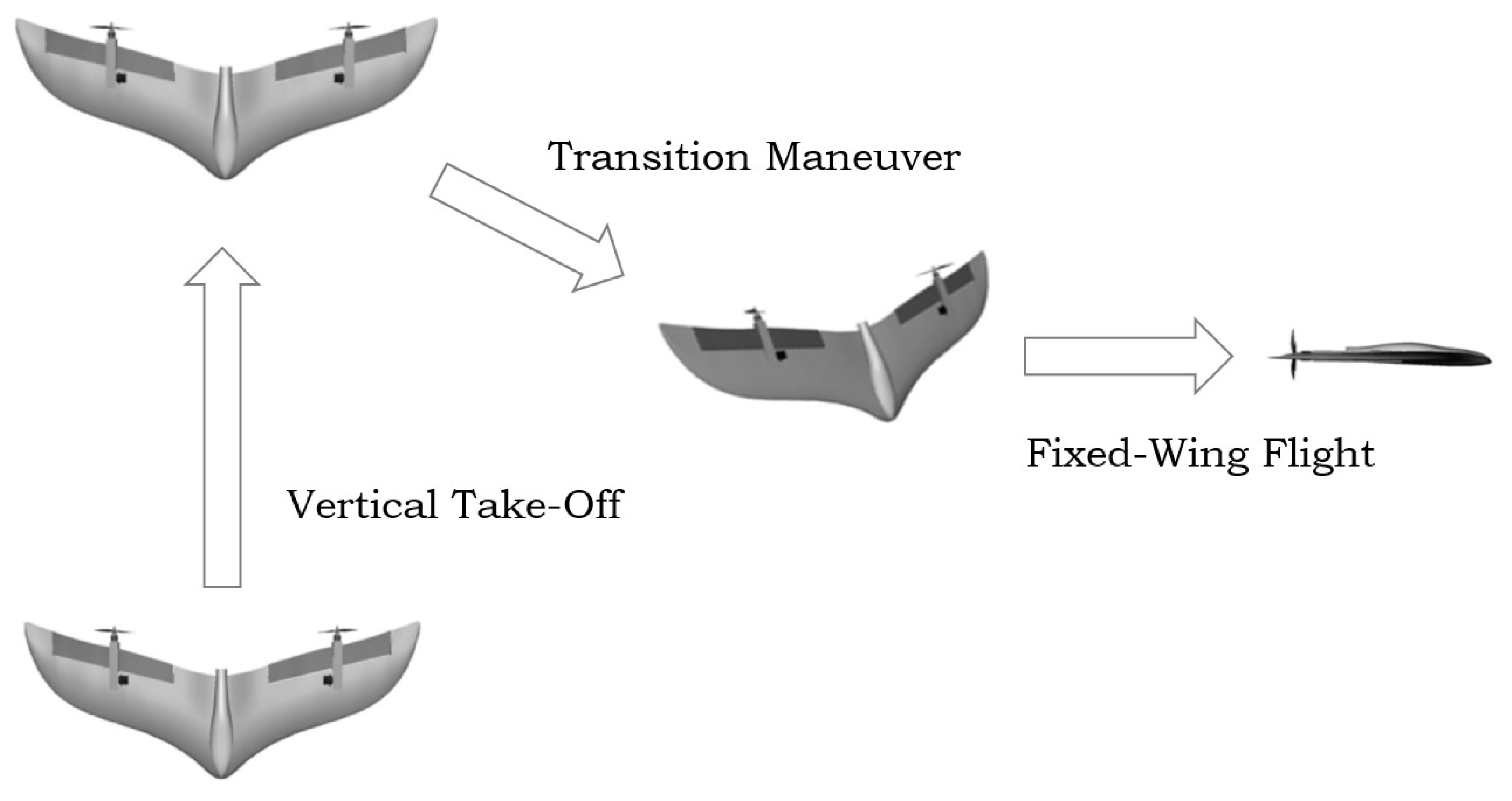
Moreover, the UAV used is the same as the previous paper, the V-Skye, a hybrid UAV categorized as a tail-sitter. This type of UAV is characterized by take-off and landing on its nose, and to perform the transition to a horizontal flight, it changes the sense of rotation of its rotors. A description of this transition maneuver may be seen in Figure 1.

To control the flight both in vertical and horizontal configuration, the V-Skye only relies on two tilting rotors and the control of the throttle of each of them. With only these flight controls, the UAV will be capable of performing a complete take-off, VTOL, transition and Fixed-wing flight. The control system’s design is based not only on simulations but also on an experimental procedure in which the controllers have to adequately stabilize the UAV, allowing it to hover and filter external disturbances. In order to control the attitude, the vehicle is provided with two tilting rotors that allow alterations of its pitch angle and yaw rate, as well as modifications in the motor throttles in order to handle roll and vertical speed variables.

From a control point of view, different types of controllers can be designed for UAVs. The simplest ones are linear PIDs based on linearized models of UAVs. In the literature, it is possible to find several approaches which solve the problem of controlling non-linear UAVs: non-linear PID-based solutions [11,12,13], non-linear robust approaches [14,15,16], back-stepping algorithms [17,18,19], sliding mode control [14,19], $H\infty$ control [18], or non-linear observer based [20,21].

On the other hand, a wide range of studies have explored the design and control of fixed-wing UAVs with tilt rotors. Some contributions are ref. [22], focused on the mechanical analysis and control system design of a tilting tri-rotor UAV; ref. [23], developing and testing quadrotors with tilt rotors and fixed wings; ref. [24], introducing a ducted-fan tilt-rotor UAV with three flight modes, including a fixed-wing mode, and using the Digital DATCOM program to calculate the stability and control derivatives; or ref. [25], where an LQR control scheme for position and yaw control in introduced, as well as a PID controller for attitude and altitude stabilization.

Finally, a more recent study can be found in the literature for the critical maneuver for the transition between VTOL and fixed-wing flight on tilt-rotor aircraft. For example, in ref. [26,27], the use of model predictive control (MPC) and back-stepping control, respectively, is discussed in order to guarantee a stable transition. An alternative to this transition is presented in ref. [28], introducing a pitch-decoupled system that allows for independent control of the tilt-rotor pitch, simplifying the transition process. Also, in ref. [29], a passively coupled tilt-rotor aircraft that uses differential thrust for transition is proposed, with a cascaded control architecture for inner-loop control. More recent contributions, such as ref. [27,30,31], deal with the challenging aim of meeting smooth and stable transitions between VTOL and fixed-wing flight on tilt-rotor aircraft.

Therefore, as mentioned before, the main goal of this work is to develop a control algorithm that allows the V-Skye to perform a VTOL, fixed-wing flight mission, along with a transition between both of them. For this purpose, the control algorithm is composed of four cascade controls with two linear PIDs each to achieve stability and navigation in each of the flight configurations.

The structure that will be followed for the rest of the article to describe the control scheme proposed is as follows: First, Section 2 will cover the description of the model for the V-Skye, including its aerodynamics, Section 3 will focus on the mathematical details that describe the V-Skye’s flight. Section 4 will cover the control algorithm for the VTOL and fixed-wing flight, along with the transition maneuver. In Section 5, the simulation platform will be described to test the control design. And, lastly, in Section 6, we discuss the results of the control design via a complete V-Skye’s flight mission: take-off, VTOL, transition and fixed-wing flight.

2. Airframe Description

In general terms, any rigid body moving in a three-dimensional (3D) space has six degrees of freedom (6DoF). With this in mind, for a body to be driven to an arbitrary position with an arbitrary orientation, six independent coordinates are needed to describe the location and the attitude of the body.

As previously discussed in ref. [10], a hovering position in equilibrium is achieved through a constant reference position with a constant heading angle. This makes it such that four of the degrees-of-freedom of the system are to be controlled according to a reference value. The other two are dependent variables that will evolve along time accordingly.

This was considered for the hover (VTOL) flight. In addition, the equilibrium horizontal (fixed-wing) flight is achieved through a constant altitude, bearing and airspeed. This case is equal as before, where four of the degrees of freedom of the system will be controlled according to a reference value, while the other two will vary dependently on the others along time.

In Figure 2, a diagram with all the references frames used is given for the V-Skye.

The V-Skye is designed with two tilting rotors, which are moved by servo-mechanisms. This results in an aircraft capable of not only modifying the thrust of each of the rotors independently but also to be turned with one degree of freedom. Moreover, the design choice for the rotors arises in additional reference frames to take into account when modeling the flight of the V-Skye. This section will be focused on the description and characteristics of the reference frames on the V-Skye, and the next one will cover the mathematical details, along with the aerodynamics of the aircraft.

2.1. Inertial Reference Frame

The first reference frame to be discussed will be the Inertial Reference Frame , represented by $\left\{{\widehat{X}}_E,{\widehat{Y}}_E,{\widehat{Z}}_E\right\}$. This represents the stationary reference system, with origin on the take-off point. It is based on the NED frame (North–East–Down) stuck at the Earth’s surface.

This system will result in the navigation position for the V-Skye, as it represents the absolute position of the UAV. Also, it will be the relation with this frame and the Body Reference System that will define the attitude coordinates of the UAV.

2.2. Body Reference Frame

The following frame is the Body Reference Frame , stuck at the aircraft center of gravity. It is represented by $\left\{{\widehat{X}}_B,{\widehat{Y}}_B,{\widehat{Z}}_B\right\}$. In this frame, the ${\widehat{X}}_B$ axis will point in the forward direction, the ${\widehat{Z}}_B$ will point downwards, and the ${\widehat{Y}}_B$ will be perpendicular to both of them, pointing to the right wing. The axes of this frame have been chosen this way according to the general convention depicted in the flight mechanics for aircraft.

The attitude coordinates relating the Body Reference Frame and the Inertial Reference Frame will be discussed in Section 3, as it will be seen that there is not a unique set of attitude coordinates.

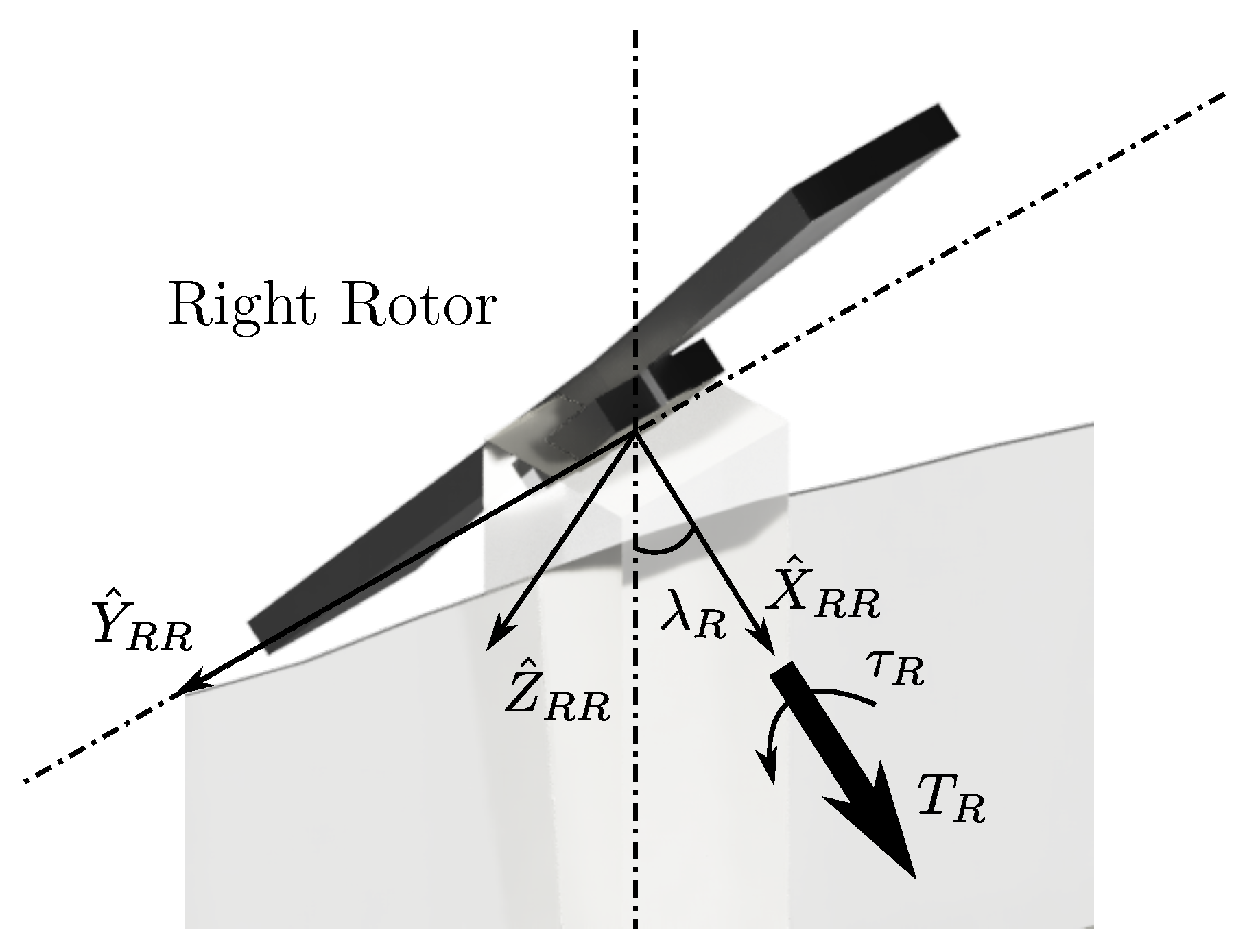
2.3. Right Rotor Frame

This frame results from the existence of rotor-tilting capabilities. It is composed of the right rotor, its propeller, and the servo-mechanism responsible for the right tilting angle (${\lambda }_R$). It is represented by $\left\{{\widehat{X}}_{RR},{\widehat{Y}}_{RR},{\widehat{Z}}_{RR}\right\}$ (see Figure 3). This frame has its center in the intersection between the rotor joint and the body shaft.

As it may be seen in Figure 3, in this frame, the ${\widehat{X}}_{RR}$ points forward and the ${\widehat{Y}}_{RR}$ is parallel to the ${\widehat{Y}}_B$ axis from the Body Reference Frame. The third axis ${\widehat{Z}}_{RR}$ is perpendicular to these two, pointing downwards. This frame is rotated with respect to the Y axis, with a tilting angle equal to ${\lambda }_R$. When there is not any tilting angle, ${\lambda }_R=0$; this frame is parallel to the Body Reference Frame . Through this design choice, the rotor thrust and torque is applied on the ${\widehat{X}}_{RR}$ axis, changed in direction by a servomotor actuating on the ${\lambda }_R$ value.

2.4. Left Rotor Frame

This frame, as with the previous one, results also from the movement of the tilting rotors. It is composed, as before, of the left rotor, its propeller, and the servo-mechanism capable of changing the tilting angle (${\lambda }_L$). It is represented by $\left\{{\widehat{X}}_{LR},{\widehat{Y}}_{LR},{\widehat{Z}}_{LR}\right\}$ (see Figure 4). Again, the origin of this frame is in the intersection between the rotor joint and the body shaft.

As it can be seen in Figure 4, in this frame, the ${\widehat{X}}_{LR}$ points in the forward direction, and the ${\widehat{Y}}_{LR}$ is parallel once again to the ${\widehat{Y}}_B$ axis from the Body Reference Frame. The third axis ${\widehat{Z}}_{LR}$ is perpendicular to these two, pointing downward. This frame is rotated with respect to the Y axis, with a tilting angle equal to ${\lambda }_L$. When the rotor is not tilted, ${\lambda }_L=0$; this frame is completely parallel to the Body Reference Frame. Through this design choice, the rotor thrust and torque are applied on the ${\widehat{X}}_{LR}$ axis, changed in direction by a servomotor by manipulating the ${\lambda }_L$ value.

2.5. Reference Frames Relation

The last part of this section is the description of the relationships among the different reference frames used for the V-Skye.

First, both the rotor frames are related to the Body Reference Frame through a pure rotation of the Y axis, described by $R_y\left(\alpha \right)$. Then, between the Body Reference Frame and the Inertial Reference Frame , they are related by an Attitude Matrix $\left[BE\right]$, which is defined by the attitude coordinates for the flight. This matrix may be defined depending on the attitude coordinates relating the body reference frame and the inertial frame (Euler angles, quaternions, etc.).

3. Mathematical Model

With the reference frames defined for the V-Skye, the assumptions considered in the derivation of the 6-DoF model are the same as [10], which are as follows:

(1)

The aircraft is assumed as a rigid body, meaning that the distance between any two point masses remains constant, without deformations. This simplifies the movement of the V-Skye to a translation and rotations around the center of mass.

(2)

The changes in the rotor’s tilting angles, ${\lambda }_R$ and ${\lambda }_L$, do not change the mass distribution.

(3)

The rotational movement of the Earth is depreciated with respect to the accelerations on the vehicle, that is, the Earth frame is an inertial frame of reference.

(4)

The atmosphere is assumed to be without wind nor turbulence.

(5)

The V-Skye has a symmetry plane at $Y_b=0$. The result is that the inertia products about this plane are $I_{y_b{x}_b}=I_{y_b{z}_b}=0$.

(6)

The aerodynamic forces are considered to be applied directly on the Body Reference Frame, as the flight speed is low, so it is the flight path angle, so it is not needed to define a Wind Reference Frame.

(7)

The rotors lie co-planar to the V-Skye’s center of gravity, adding no vertical thrust torque.

3.1. Translational Equations

Given $\overrightarrow{F}$ as the resultant sum of forces acting on the system, m is the aircraft total mass and $\overrightarrow{V}$ is the aircraft linear velocity with respect to the inertial frame (E). To derive the translational equations, Newton’s second law is used, which may be written as:

$$\begin{array}{cc}\hfill \overrightarrow{F}& =m·\dot{\overrightarrow{V}}\hfill \end{array}$$

(1)

$$\begin{array}{cc}\hfill \{F_{x_b},F_{y_b},F_{z_b}\}& =m·\frac{{ }^{E}d}{dt}\left(\{u,v,w\}\right)\hfill \end{array}$$

(2)

where $F_{x_b}$, $F_{y_b}$ and $F_{z_b}$ are the three components of the resultant force. u, v and w are the system linear velocities. Both of these magnitudes are expressed from the Body Reference Frame. Using the Transport Theorem, the linear velocity’s inertial time derivative may be expressed as the sum of the body time derivative plus the cross product between the linear and angular velocities:

$$\begin{array}{cc}\hfill \dot{\overrightarrow{V}}& =\frac{{ }^{B}d}{dt}\left(\{u,v,w\}\right){+}^E{\overrightarrow{\omega }}^B\times \overrightarrow{V}\hfill \end{array}$$

(3)

$$\begin{array}{cc}\hfill \dot{\overrightarrow{V}}& =\{\dot{u},\dot{v},\dot{w}\}+\{p,q,r\}\times \{u,v,w\}\hfill \end{array}$$

(4)

$$\begin{array}{cc}\hfill \dot{\overrightarrow{V}}& =\{\dot{u}+q·w-r·v,\dot{v}+r·u-p·w,\dot{w}+p·v-q·u\}\hfill \end{array}$$

(5)

where ${ }^E{\overrightarrow{\omega }}^B$ corresponds to the angular velocity at which the Body Reference Frame rotates with respect to the Inertial Reference Frame, with p, q, and r as its components, measured from the Body Reference Frame. With this, the components of vector Equation (1) may be separated as:

$$\begin{array}{cc}\hfill m·(\dot{u}+q·w-r·v)& =F_{x_b}\hfill \end{array}$$

(6)

$$\begin{array}{cc}\hfill m·(\dot{v}+r·u-p·w)& =F_{y_b}\hfill \end{array}$$

(7)

$$\begin{array}{cc}\hfill m·(\dot{w}+p·v-q·u)& =F_{z_b}\hfill \end{array}$$

(8)

The forces acting on the V-Skye may be split up into the gravitational force, the aerodynamic force, and the rotors’ thrust contribution:

$$\overrightarrow{F}={\overrightarrow{F}}_g+{\overrightarrow{F}}_a+{\overrightarrow{F}}_T$$

(9)

First, the gravitational force is generally measured from the Inertial Reference Frame, so it has to be expressed with respect to the Body Reference Frame, using the Attitude Matrix ($\left[BE\right]$):

$${\overrightarrow{F}}_g=\left[BE\right]·\{0,0,m·g\}$$

(10)

For the rotors’ thrust, $T_R$ and $T_L$ are the thrust magnitudes for the right and left rotors, respectively. These forces are expressed in magnitude in each respective rotor’s frame. What has to be done is to apply the rotation given by the tilting mechanisms. So, the force magnitudes must be projected using the tilting angles’ rotation (${\lambda }_R$ and ${\lambda }_L$):

$$\begin{array}{cc}\hfill {\overrightarrow{T}}_R& =T_R·\{cos\left({\lambda }_R\right),0,-sin\left({\lambda }_L\right)\}\hfill \end{array}$$

(11)

$$\begin{array}{cc}\hfill {\overrightarrow{T}}_L& =T_L·\{cos\left({\lambda }_L\right),0,-sin\left({\lambda }_L\right)\}\hfill \end{array}$$

(12)

In ref. [10], a study is presented of the performance for several types of propellers at different airflow conditions. Also presented is a model for rotor thrust and torque at a low Reynolds number, convenient for the V-Skye’s flight conditions. Having T and $\tau$ represent the rotor’s thrust and torque and $C_T$ and $C_{\tau }$ as the force and torque coefficients, respectively, it may be expressed that:

$$\begin{array}{cc}\hfill T& =C_T\rho n^2{D}^4\hfill \end{array}$$

(13)

$$\begin{array}{cc}\hfill \tau & =C_{\tau }\rho n^2{D}^5\hfill \end{array}$$

(14)

where n is the angular velocity of the rotor, $\rho$ is the air density, and D is the blade diameter. So, the relation between thrust and torque is written as:

$$T=\frac{C_T}{D·C_{\tau }}\tau$$

(15)

As a matter of simplicity, the thrust and torque will be expressed using a proportional relation between these quantities and the throttle level. They will be related using constant values, represented by $k_T$ and $k_{\tau }$ for the thrust and torque, respectively. Symbolizing ${\delta }_R$ and ${\delta }_L$ as the rotors’ throttle, taking into account the electronic speed controllers mounted with the brushless DC motors, the torques may be expressed as:

$$\begin{array}{cc}\hfill {\tau }_R& =k_{\tau }·{\delta }_R\hfill \end{array}$$

(16)

$$\begin{array}{cc}\hfill {\tau }_L& =k_{\tau }·{\delta }_L\hfill \end{array}$$

(17)

So, the rotors’ thrust dependence with the throttle is:

$$\begin{array}{cc}\hfill T_R& =\frac{C_T}{D·C_{\tau }}{k}_{\tau }·{\delta }_R=k_T·{\delta }_R\hfill \end{array}$$

(18)

$$\begin{array}{cc}\hfill T_L& =\frac{C_T}{D·C_{\tau }}{k}_{\tau }·{\delta }_L=k_T·{\delta }_L\hfill \end{array}$$

(19)

where $k_{\tau }$ is the torque’s throttle coefficient, constant for a given motor and speed controller, and $k_T$ is the thrust’s throttle coefficient, considered constant for the equilibrium flight (although it is dependent on the flight airspeed). As a result, the final V-Skye’s thrust contribution is given by:

$${\overrightarrow{F}}_T={\overrightarrow{T}}_R+{\overrightarrow{T}}_L=\{F_{T_x},F_{T_y},F_{T_z}\}$$

(20)

whose components are:

$$\begin{array}{cc}\hfill F_{T_x}& =k_T·{\delta }_R·cos\left({\lambda }_R\right)+k_T·{\delta }_L·cos\left({\lambda }_L\right)\hfill \end{array}$$

(21)

$$\begin{array}{cc}\hfill F_{T_y}& =0\hfill \end{array}$$

(22)

$$\begin{array}{cc}\hfill F_{T_z}& =-k_T·{\delta }_R·sin\left({\lambda }_R\right)-k_T·{\delta }_L·sin\left({\lambda }_L\right)\hfill \end{array}$$

(23)

Finally, the aerodynamic forces are formed by the lift and drag force. As it is considered to be applied on the Body Reference Frame directly, the aerodynamic vector force may be expressed as:

$${\overrightarrow{F}}_a=\{-Drag,0,-Lift\}$$

(24)

where the lift and drag will be expressed as

$$\begin{array}{cc}\hfill Lift& =\frac{1}{2}\rho V^{2}SCL\approx \frac{1}{2}\rho u^{2}SCL\hfill \end{array}$$

(25)

$$\begin{array}{cc}\hfill Drag& =\frac{1}{2}\rho V^{2}SCD\approx \frac{1}{2}\rho u^{2}SCD\hfill \end{array}$$

(26)

where $\rho$ is the air density, V is the flight airspeed, S is the wing reference area, and $CL$ and $CD$ represent the lift and drag coefficients. In addition, the airspeed is approximated to be the linear velocity in the forward direction, as the vertical and transversal velocity in a fixed-wing configuration will be negligible.

3.2. Rotational Equations

For the rotational equations, first, the angular momentum has to be defined around the V-Skye’s center of gravity:

$${\overrightarrow{H}}^{c.g}={\left[\begin{array}{ccc}{I}_{x_b{x}_b}& -I_{x_b{y}_b}& -I_{x_b{z}_b}\\ -I_{y_b{x}_b}& I_{y_b{y}_b}& -I_{y_b{z}_b}\\ -I_{z_b{x}_b}& -I_{z_b{x}_b}& -I_{z_b{z}_b}\end{array}\right]}^{c.g}{·}^E{\overrightarrow{\omega }}^B$$

(27)

where $I_{ii}\forall i\in \{x_b,y_b,z_b\}$ correspond to the moments of inertia around the center of gravity, and $I_{ij}\forall ij\in \{x_b,y_b,z_b\}$, with $i\ne j$ corresponding to the products of inertia.

With the angular momentum defined, the rotational equations may be expressed as the Newton’s Second Law of Rotations, in combination with the Transport Theorem, which states that:

$$\begin{array}{cc}\hfill {\overrightarrow{Q}}^{c.g}& =\{L,M,N\}={\dot{\overrightarrow{H}}}^{c.g}\hfill \end{array}$$

(28)

$$\begin{array}{cc}\hfill {\overrightarrow{Q}}^{c.g}& =\{L,M,N\}=\frac{{ }^{B}d}{dt}\left({\overrightarrow{H}}^{c.g}\right){+}^E{\overrightarrow{\omega }}^B\times {\overrightarrow{H}}^{c.g}\hfill \end{array}$$

(29)

where ${\overrightarrow{Q}}^{c.g}$ represents the total external moment applied on the center of gravity, measured from the Body Reference Frame, whose components are L, M, and N. Following the same steps as before, this vectorial equations may be divided among their components:

$$\begin{array}{cc}\hfill L& =I_{xx}\dot{p}-I_{xz}\dot{r}-I_{xz}pq+(I_{zz}-I_{yy})qr\hfill \end{array}$$

(30)

$$\begin{array}{cc}\hfill M& =I_{yy}\dot{q}-I_{xz}(p^2-r^2)+(I_{xx}-I_{zz})pr\hfill \end{array}$$

(31)

$$\begin{array}{cc}\hfill N& =I_{zz}\dot{r}-I_{xz}\dot{p}+I_{xz}rq+(I_{yy}-I_{xx})pq\hfill \end{array}$$

(32)

Same as the external forces, the external torques applied to the V-Skye may be divided on the thrust and the aerodynamic torque:

$${\overrightarrow{Q}}^{c.g}={\overrightarrow{Q}}_T^{c.g}+{\overrightarrow{Q}}_a^{c.g}$$

(33)

On the one hand, for the rotors’ contribution to the torque, it may be sub-divided also in the moment introduced by the thrust and the one by its own torque:

$$\begin{array}{cc}\hfill {\overrightarrow{Q}}_T^{c.g}& ={\overrightarrow{Q}}_{m_R}+{\overrightarrow{Q}}_{m_L}\hfill \end{array}$$

(34)

$$\begin{array}{cc}\hfill {\overrightarrow{Q}}_{m_R}& ={\overrightarrow{r}}_{m_R}\times {\overrightarrow{T}}_R+{\overrightarrow{\tau }}_R\hfill \end{array}$$

(35)

$$\begin{array}{cc}\hfill {\overrightarrow{Q}}_{m_L}& ={\overrightarrow{r}}_{m_L}\times {\overrightarrow{T}}_L+{\overrightarrow{\tau }}_L\hfill \end{array}$$

(36)

The moment of the rotors’ thrust may be calculated as:

$$\begin{array}{cc}\hfill {\overrightarrow{r}}_{m_R}\times {\overrightarrow{T}}_R& =\{-x_{m_R},y_{m_R},0\}\times \left(k_T{\delta }_R\{cos\left({\lambda }_R\right),0,-sin\left({\lambda }_R\right)\}\right)\hfill \end{array}$$

(37)

$$\begin{array}{cc}\hfill & =k_T{\delta }_R·\{-y_{m_R}sin\left({\lambda }_R\right),-x_{m_R}sin\left({\lambda }_R\right),-y_{m_R}cos\left({\lambda }_R\right)\}\hfill \end{array}$$

(38)

$$\begin{array}{cc}\hfill {\overrightarrow{r}}_{m_L}\times {\overrightarrow{T}}_L& =\{-x_{m_L},-y_{m_L},0\}\times \left(k_T{\delta }_L\{cos\left({\lambda }_L\right),0,-sin\left({\lambda }_L\right)\}\right)\hfill \end{array}$$

(39)

$$\begin{array}{cc}\hfill & =k_T{\delta }_L·\{y_{m_L}sin\left({\lambda }_L\right),-x_{m_L}sin\left({\lambda }_L\right),y_{m_L}cos\left({\lambda }_L\right)\}\hfill \end{array}$$

(40)

In addition, the contribution generated by the rotor’s torque may be calculated as:

$$\begin{array}{cc}\hfill {\overrightarrow{\tau }}_R& ={\tau }_R·\left\{cos\left({\lambda }_R\right),0,-sin\left({\lambda }_R\right)\right\}=k_{\tau }{\delta }_R·\left\{cos\left({\lambda }_R\right),0,-sin\left({\lambda }_R\right)\right\}\hfill \end{array}$$

(41)

$$\begin{array}{cc}\hfill {\overrightarrow{\tau }}_L& ={\tau }_L·\left\{-cos\left({\lambda }_L\right),0,sin\left({\lambda }_L\right)\right\}=k_{\tau }{\delta }_L·\left\{-cos\left({\lambda }_L\right),0,sin\left({\lambda }_L\right)\right\}\hfill \end{array}$$

(42)

So, the final rotor’s total contribution to the V-Skye’s torque is:

$$\begin{array}{cc}\hfill {\overrightarrow{Q}}_{m_R}& ={\delta }_R\left(k_T·\{-y_{m_R}sin\left({\lambda }_R\right),-x_{m_R}sin\left({\lambda }_R\right),-y_{m_R}cos\left({\lambda }_R\right)\}\right.\hfill \\ \hfill & \left.+k_{\tau }·\{cos\left({\lambda }_R\right),0,-sin\left({\lambda }_R\right)\}\right)\hfill \end{array}$$

(43)

$$\begin{array}{cc}\hfill {\overrightarrow{Q}}_{m_L}& ={\delta }_L\left(k_T·\{y_{m_L}sin\left({\lambda }_L\right),-x_{m_L}sin\left({\lambda }_L\right),y_{m_L}cos\left({\lambda }_L\right)\}\right.\hfill \\ \hfill & \left.+k_{\tau }·\{-cos\left({\lambda }_L\right),0,sin\left({\lambda }_L\right)\}\right)\hfill \end{array}$$

(44)

On the other hand, for the aerodynamic torque, it may be calculated as:

$$\begin{array}{cc}\hfill {\overrightarrow{Q}}_a^{c.g}& =\left\{-x_{AC},0,0\right\}\times \left\{-Drag,0,-Lift\right\}=\left\{0,-Lift{x}_{AC},0\right\}=\hfill \end{array}$$

(45)

$$\begin{array}{cc}\hfill & \left\{0,-\frac{1}{2}\rho u^{2}SCL{x}_{AC},0\right\}\hfill \end{array}$$

(46)

3.3. Kinematic Rotational Equations

An additional aspect to consider is the equations that will govern the attitude coordinates. In ref. [10], the Euler Angles coordinate set was used, specifically, a (3-2-1) Euler Angles set, representing the three basic movements of an aircraft: roll ($\varphi$), pitch ($\theta$), and yaw ($\psi$).

Before entering the mathematical model, in Figure 5, the Attitude Matrix is specified, responsible for relating the Body Reference Frame and the Inertial Reference Frame. Taking the Euler Angles as attitude coordinates, this matrix takes the following form:

$$\left[BE\right]=\left[\begin{array}{ccc}c\left(\psi \right)c\left(\theta \right)& c\left(\theta \right)s\left(\psi \right)& -s\left(\theta \right)\\ c\left(\psi \right)s\left(\varphi \right)s\left(\theta \right)-c\left(\varphi \right)s\left(\psi \right)& c\left(\varphi \right)c\left(\psi \right)+s\left(\varphi \right)s\left(\psi \right)s\left(\theta \right)& c\left(\theta \right)s\left(\varphi \right)\\ s\left(\varphi \right)s\left(\psi \right)c\left(\varphi \right)c\left(\psi \right)s\left(\theta \right)& c\left(\varphi \right)s\left(\psi \right)s\left(\theta \right)-c\left(\psi \right)s\left(\varphi \right)& c\left(\varphi \right)c\left(\theta \right)\end{array}\right]$$

(47)

taking into account that $c\left(\alpha \right)=cos\left(\alpha \right)$ and $s\left(\alpha \right)=sin\left(\alpha \right)$. In addition, we need the differential equation which governs the rate of change for the roll, pitch, and yaw:

$$\left[\begin{array}{c}\dot{\psi }\\ \dot{\theta }\\ \dot{\varphi }\end{array}\right]=\frac{1}{c\left(\theta \right)}\left[\begin{array}{ccc}0& s\left(\varphi \right)& c\left(\varphi \right)\\ 0& c\left(\varphi \right)c\left(\theta \right)& -s\left(\varphi \right)c\left(\theta \right)\\ c\left(\theta \right)& s\left(\varphi \right)s\left(\theta \right)& c\left(\varphi \right)s\left(\theta \right)\end{array}\right]$$

(48)

This was the approach for ref. [10]. Nevertheless, in this article, the problem for both VTOL and cruise flight is tackled, thus making this set of coordinates not adequate for the numerical simulation, as it presents a singularity when $\theta =\pm 90°$. Taking into account that one of the flight operations is at this particular angle, they are not adequate to simulate the complete flight envelope.

With this, we propose the use of quaternions. They are a set of four attitude coordinates $(q_0,q_1,q_2,q_3)$ which are capable of representing the 3D orientation of the body. The Attitude Matrix will be:

$$\begin{array}{c}\hfill \left[BE\right]=\left[\begin{array}{ccc}{q}_0^2+q_1^2-q_2^2-q_3^2& 2(q_1{q}_2+q_0{q}_3)& 2(q_1{q}_3-q_0{q}_2)\\ 2(q_1{q}_2-q_0{q}_3)& q_0^2-q_1^2+q_2^2-q_3^2& 2(q_2{q}_3+q_0{q}_1)\\ 2(q_1{q}_3+q_0{q}_2)& 2(q_2{q}_3-q_0{q}_1)& q_0^2-q_1^2-q_2^2+q_3^2\end{array}\right]\end{array}$$

(49)

The differential equation is:

$$\begin{array}{c}\hfill \left[\begin{array}{c}{\dot{q}}_0\\ {\dot{q}}_1\\ {\dot{q}}_2\\ {\dot{q}}_3\end{array}\right]=\frac{1}{2}\left[\begin{array}{cccc}{q}_0& -q_1& -q_2& -q_3\\ q_1& q_0& -q_3& q_2\\ q_2& q_3& q_0& -q_1\\ q_3& -q_2& q_1& q_0\end{array}\right]\left[\begin{array}{c}0\\ p\\ q\\ r\end{array}\right]\end{array}$$

(50)

This approach solves the inconvenience of the mathematical singularity, as they are an adequate set of coordinates. Nevertheless, a new problem arises, as they are not adequate for representing and controlling the attitude of the V-Skye. Euler angles are a better option, as they are a more intuitive set of coordinates. So, the final solution will be using quaternions for the internal numerical simulation and Euler angles for output and the feedback control.

The (3-2-1) Euler angles will be used for the cruise flight, and a special set of angles will be built for the VTOL flight, called Vertical Euler angles [32]. In the latter case, we use a (1-2-3) Euler angles set:

• Start at a vertical attitude position, that is, with the V-Skye in a VTOL position.
• First, apply a rotation around the ${\widehat{X}}_b$ axis rotation, which is the vertical roll angle (${\varphi }_v$).
• Then, perform a second rotation around the new ${\widehat{Y}}_b$ axis, which is the vertical pitch angle (${\theta }_v$).
• Lastly, execute a third rotation around the new ${\widehat{Z}}_b$, which is the vertical yaw angle (${\psi }_v$).

Then, the Attitude Matrix will be:

$$\left[BE\right]=\left[\begin{array}{ccc}-c\left({\psi }_v\right)s\left({\theta }_v\right)c\left({\varphi }_v\right)+s\left({\psi }_v\right)s\left({\varphi }_v\right)& c\left({\psi }_v\right)s\left({\theta }_v\right)s\left({\varphi }_v\right)+s\left({\psi }_v\right)c\left({\varphi }_v\right)& -c\left({\psi }_v\right)c\left({\theta }_v\right)\\ s\left({\psi }_v\right)s\left({\theta }_v\right)c\left({\varphi }_v\right)+c\left({\psi }_v\right)s\left({\varphi }_v\right)& -s\left({\psi }_v\right)s\left({\theta }_v\right)s\left({\varphi }_v\right)+c\left({\psi }_v\right)c\left({\varphi }_v\right)& s\left({\psi }_v\right)c\left({\theta }_v\right)\\ c\left({\theta }_v\right)c\left({\varphi }_v\right)& -c\left({\theta }_v\right)s\left({\varphi }_v\right)& -s\left({\theta }_v\right)\end{array}\right]$$

(51)

Then, coordinate transformation between the quaternions and these Euler Angles will be used for the visual representation of the orientation.

3.4. Collection of Non-Linear Equations

In addition to the equations derived before, the kinematic equations are added, responsible for the navigation of the V-Skye. As a summary, the aircraft model is represented by the following set of equations:

• Translational Dynamic Equations

  $$\begin{array}{cc}\hfill \dot{u}& =rv-qw+2g(q_1{q}_3-q_0{q}_2)+\hfill \end{array}$$

  $$\begin{array}{cc}\hfill & \frac{1}{m}\left(k_T{\delta }_{L}cos\left({\lambda }_L\right)-\frac{1}{2}\rho u^2{S}_w^{2}CD+k_T{\delta }_{R}cos\left({\lambda }_R\right)\right)\hfill \end{array}$$

  (52)

  $$\begin{array}{cc}\hfill \dot{v}& =pw-ru+2g(q_0{q}_1+q_2{q}_3)\hfill \\ \hfill \dot{w}& =qu-pv+g(q_0^2-q_1^2-q_2^2+q_3^2)+\hfill \end{array}$$

  (53)

  $$\begin{array}{cc}\hfill & \frac{1}{m}\left(-\frac{1}{2}\rho u^2{S}_{w}CL-k_T{\delta }_{L}sin\left({\lambda }_L\right)-k_T{\delta }_{R}sin\left({\lambda }_R\right)\right)\hfill \end{array}$$

  (54)
• Rotational Dynamic Equations

  $$\begin{array}{cc}\hfill \dot{p}-\frac{I_{xz}}{I_{xx}}\dot{r}& =\frac{I_{zx}}{I_{xx}}qr+\frac{I_{yy}-I_{zz}}{I_{xx}}qr+\frac{{\delta }_R}{I_{xx}}\left(k_{\tau }cos\left({\lambda }_R\right)-k_T{y}_{m_R}cos\left({\lambda }_R\right)\right)\hfill \end{array}$$

  $$\begin{array}{cc}\hfill & -\frac{{\delta }_L}{I_{xx}}\left(k_{\tau }cos\left({\lambda }_R\right)-k_T{y}_{m_L}cos\left({\lambda }_L\right)\right)\hfill \\ \hfill \dot{q}& =\frac{I_{xz}}{I_{yy}}\left(p^2-r^2\right)+\frac{I_{zz}-I_{xx}}{I_{yy}}pr\hfill \end{array}$$

  (55)

  $$\begin{array}{cc}\hfill & -\frac{1}{I_{yy}}Lift{x}_{AC}-\frac{1}{I_{yy}}{\delta }_L{k}_T{x}_{m_L}sin\left({\lambda }_L\right)-\frac{1}{I_{yy}}{\delta }_R{k}_T{x}_{m_R}sin\left({\lambda }_R\right)\hfill \\ \hfill \dot{r}-\frac{I_{zx}}{I_{zz}}& =-\frac{I_{xz}}{I_{zz}}qr+\frac{I_{xx}-I_{yy}}{I_{zz}}pq+\frac{{\delta }_L}{I_{zz}}\left(k_{\tau }sin\left({\lambda }_L\right)+k_T{y}_{m_L}cos\left({\lambda }_L\right)\right)\hfill \end{array}$$

  (56)

  $$\begin{array}{cc}\hfill & -\frac{{\delta }_R}{I_{zz}}\left(k_{\tau }sin\left({\lambda }_R\right)+k_T{y}_{m_R}cos\left({\lambda }_R\right)\right)\hfill \end{array}$$

  (57)
• Kinematic Rotational Equations

  $$\begin{array}{cc}\hfill u& ={\dot{x}}_e(q_0^2+q_1^2-q_2^2-q_3^2)+2{\dot{y}}_e(q_1{q}_2+q_0{q}_3)+2{\dot{z}}_e(-q_0{q}_2+q_1{q}_3)\hfill \end{array}$$

  (58)

  $$\begin{array}{cc}\hfill v& =2{\dot{x}}_e(q_1{q}_2-q_0{q}_3)+{\dot{y}}_e(q_0^2-q_1^2+q_2^2-q_3^2)+2{\dot{z}}_e(q_0{q}_1+q_2{q}_3)\hfill \end{array}$$

  (59)

  $$\begin{array}{cc}\hfill w& =2{\dot{x}}_e(q_0{q}_2+q_1{q}_3)+2{\dot{y}}_e(-q_0{q}_1+q_2{q}_3)+{\dot{z}}_e(q_0^2-q_1^2-q_2^2+q_3^2)\hfill \end{array}$$

  (60)
• Kinematic Translational Equations (Quaternions)

  $$\begin{array}{cc}\hfill {\dot{q}}_0& =\frac{1}{2}(-p{q}_1-q{q}_2-r{q}_3)\hfill \end{array}$$

  (61)

  $$\begin{array}{cc}\hfill {\dot{q}}_1& =\frac{1}{2}(p{q}_0-q{q}_3+r{q}_2)\hfill \end{array}$$

  (62)

  $$\begin{array}{cc}\hfill {\dot{q}}_2& =\frac{1}{2}(p{q}_3+q{q}_0-r{q}_1)\hfill \end{array}$$

  (63)

  $$\begin{array}{cc}\hfill {\dot{q}}_3& =\frac{1}{2}(-p{q}_2+q{q}_1+r{q}_0)\hfill \end{array}$$

  (64)

4. Control Design

Regarding the control design, it presents several challenges to face. The complexity of flight dynamics comes from the non-linearity of the system, the unstable nature of the UAV, the transition flight phase, and the high coupling among the equations. In addition, in the case of the V-Skye, the system is under-actuated, as there are only four control inputs to be used for the entire flight envelope (take-off, transition, cruise, etc.). For this reason, a robust and reliable feedback control strategy is needed to achieve a stable flight within the flight envelope.

Before the proposed control scheme, taking a look at the non-linear equations of motion, it may be seen that a manipulation on one of the four system inputs, ${\delta }_R$, ${\delta }_L$, ${\lambda }_R$ or ${\lambda }_L$, modifies multiple state variables at the same time. This is a consequence of the high coupling of the system dynamics. With this in mind, to minimize the effect of these coupled actuators, a new set of four inputs is proposed, $u_1$, $u_2$, $u_3$ and $u_4$, which are defined as a linear combination of the real system inputs:

$$\begin{array}{cc}\hfill u_1& =\frac{1}{2}({\delta }_L-{\delta }_R)\hfill \end{array}$$

(65)

$$\begin{array}{cc}\hfill u_2& =-({\lambda }_R+{\lambda }_L)\hfill \end{array}$$

(66)

$$\begin{array}{cc}\hfill u_3& ={\lambda }_R-{\lambda }_L\hfill \end{array}$$

(67)

$$\begin{array}{cc}\hfill u_4& =\frac{1}{2}({\delta }_R+{\delta }_L)\hfill \end{array}$$

(68)

Now, with the new system inputs defined, for their simplicity, easy implementation and robustness, a decentralized and linear cascade control scheme is chosen based on four proportional–integral–derivative controllers (PIDs) to design the attitude and navigation control. This way, an Inner Loop is built that is in charge of the attitude tracking, and an Outer Loop is built that is responsible for the flight navigation. This control scheme is reflected in Figure 6.

It may be seen that this strategy relies on two controllers placed in series, where the output of the Outer Loop controller ($C_1\left(s\right)$) sets the reference for the Inner Loop controller ($C_2\left(s\right)$).

Furthermore, depending on the V-Skye’s flight state, whether it is during VTOL or cruise flight, it will have a different control scheme. The difference resides in the system state variables to be considered. Figure 7 shows the proposed control scheme for each of the configurations.

On the one hand, for the VTOL configuration, the Inner Loop is composed of a controller for each of the vertical Euler angles and one for the vertical velocity. Then, the Outer Loop will take as input the desired coordinates and will set the reference for the Inner Loop.

On the other hand, for the fixed-wing configuration, the Inner Loop is composed again of a controller for each of the normal Euler angles and one for the airspeed. For the Outer Loop, its input will be the desired bearing, altitude, and airspeed, setting the reference for the Inner Loop.

4.1. VTOL Controllers

The control scheme for the VTOL configuration is similar to that in ref. [10].

4.1.1. Vertical Euler Angles Controllers

The controllers for vertical Euler angles are implemented the same way, a standard PID controller with feedback of the corresponding estimated angle from the complementary filter, which results in the following control law:

$$\begin{array}{cc}\hfill u_1& =K_{p,1}\left(({\psi }_{v_r}-{\psi }_v)+\frac{1}{T_{i,1}}\int ({\psi }_{v_r}-{\psi }_v)dt+T_{d,1}({\dot{\psi }}_{v_r}-{\dot{\psi }}_v)\right)\hfill \end{array}$$

(69)

$$\begin{array}{cc}\hfill u_2& =K_{p,2}\left(({\theta }_{v_r}-{\theta }_v)+\frac{1}{T_{i,2}}\int ({\theta }_{v_r}-{\theta }_v)dt+T_{d,2}({\dot{\theta }}_{v_r}-{\dot{\theta }}_v)\right)\hfill \end{array}$$

(70)

$$\begin{array}{cc}\hfill u_3& =K_{p,3}\left(({\varphi }_{v_r}-{\varphi }_v)+\frac{1}{T_{i,3}}\int ({\varphi }_{v_r}-{\varphi }_v)dt+T_{d,3}({\dot{\varphi }}_{v_r}-{\dot{\varphi }}_v)\right)\hfill \end{array}$$

(71)

where $K_{p,i}$, $T_{i,i}$, and $T_{d,i}$ are, respectively, the proportional, integral, and derivative constants. Then, ${\psi }_{v,r}$, ${\theta }_{v,r}$, and ${\varphi }_{v,r}$ represent the reference vertical yaw, pitch, and roll angles. $u_i$ is the controller action, where $u_1$ represents the thrust difference between the two rotors (similar to the aircraft rudder), $u_2$ is associated with the tilt angle of both rotors (similar to the aircraft elevator), and $u_3$ represents the difference between the rotor tilting angle (similar to the aircraft ailerons).

4.1.2. Vertical Velocity Controller

Due to the high degree of coupling inside the system dynamics, any modification on the tilting angles ${\lambda }_R$ and ${\lambda }_L$ from the previous controllers will definitely add disturbances to the vertical thrust, which will affect the vertical velocity. Therefore, a controller is added for the vertical velocity as:

$$u_4=K_{p,4}\left(({\dot{z}}_{e_r}-{\dot{z}}_e)+\frac{1}{T_{i,4}}\int ({\dot{z}}_{e_r}-{\dot{z}}_e)dt+T_{d,4}({\ddot{z}}_{e_r}-{\ddot{z}}_e)\right)$$

(72)

where ${\dot{z}}_{e_r}$ is the reference altitude velocity, and ${\dot{z}}_e$ is the measured vertical velocity from the inertial magnetic unit (IMU) inside the V-Skye. The control action $u_4$ represents the increase, of the same amount, in both rotors’ thrust (similar to the aircraft throttle).

4.1.3. Navigation Controllers

For the Outer Loop controllers, responsible for the V-Skye navigation during VTOL flight, they will be implemented in the same way as the previous controllers, through a standard PID controller:

$$\begin{array}{cc}\hfill {\theta }_{v_r}& =K_{p,5}\left((x_{e_r}-x_e)+\frac{1}{T_{i,5}}\int (x_{e_r}-x_e)dt+T_{d,5}({\dot{x}}_{e_r}-{\dot{x}}_e)\right)\hfill \end{array}$$

(73)

$$\begin{array}{cc}\hfill {\psi }_{v_r}& =K_{p,6}\left((y_{e_r}-y_e)+\frac{1}{T_{i,6}}\int (y_{e_r}-y_e)dt+T_{d,6}({\dot{y}}_{e_r}-{\dot{y}}_e)\right)\hfill \end{array}$$

(74)

$$\begin{array}{cc}\hfill {\dot{z}}_{e_r}& =K_{p,7}\left((z_{e_r}-z_e)+\frac{1}{T_{i,7}}\int (z_{e_r}-z_e)dt+T_{d,7}({\dot{z}}_{e_r}-{\dot{z}}_e)\right)\hfill \end{array}$$

(75)

where $\{x_{e_r},y_{e_r},z_{e_r}\}$ is the desired Cartesian position, and $\{x_e,y_e,z_e\}$ is the measured V-Skye position.

The last Outer Loop controller, responsible for setting up the reference for the vertical roll angle, will be 0. The reason is, in this case, that it is not desired to rotate the V-Skye around its axes, so it will be forced to maintain a constant bearing angle.

4.2. Fixed-Wing Controllers

For the fixed-wing flight and the transition maneuver, as they will share the same control scheme, the implementation will be the same as the VTOL controllers, changing the state variables to control.

4.2.1. Euler Angles Controllers

The controllers for the Euler Angles are formed from a standard PID controller, with the corresponding feedback from the estimated angle, which comes from the complementary filter, resulting in:

$$\begin{array}{cc}\hfill u_1& =K_{p,1}\left(({\psi }_r-\psi )+\frac{1}{T_{i,1}}\int ({\psi }_r-\psi )dt+T_{d,1}({\dot{\psi }}_r-\dot{\psi })\right)\hfill \end{array}$$

(76)

$$\begin{array}{cc}\hfill u_2& =K_{p,2}\left(({\theta }_r-\theta )+\frac{1}{T_{i,2}}\int ({\theta }_r-\theta )dt+T_{d,2}({\dot{\theta }}_r-\dot{\theta })\right)\hfill \end{array}$$

(77)

$$\begin{array}{cc}\hfill u_3& =K_{p,3}\left(({\varphi }_r-\varphi )+\frac{1}{T_{i,3}}\int ({\varphi }_r-\varphi )dt+T_{d,3}({\dot{\varphi }}_r-\dot{\varphi })\right)\hfill \end{array}$$

(78)

where again, $K_{p,i}$, $T_{i,i}$, and $T_{d,i}$ are the proportional, integral, and derivative constants, respectively. Then, ${\psi }_r$, ${\theta }_r$, and ${\varphi }_r$ represent the reference attitude of the V-Skye (yaw, pitch, and roll). And $u_i$ is the controller action, where $u_1$ represents the thrust difference, $u_2$ is the tilt angle of both rotors, and $u_3$ is the difference between the tilting rotor angle.

4.2.2. Airspeed Controller

Apart from the attitude tracking controllers, a fourth controller is implemented that will be the flight airspeed. This controller will work both at the Inner and Outer Loop control schemes at the cascade control. Once again, the control law will be based on a standard PID:

$$u_4=K_{p,4}\left((V_r-V)+\frac{1}{T_{i,4}}\int (V_r-V)dt+T_{d,4}({\dot{V}}_r-\dot{V})\right)$$

(79)

where $V_r$ is the desired airspeed at any given moment, and V is the airspeed measured from the IMU unit.

4.2.3. Navigation Controllers

For the controllers responsible for the fixed-wing navigation, standard PIDs will be used, setting the reference for the Inner Loop controllers:

$$\begin{array}{cc}\hfill {\varphi }_r& =K_{p,5}\left(({\xi }_r-\xi )+\frac{1}{T_{i,5}}\int ({\xi }_r-\xi )dt+T_{d,5}({\dot{\xi }}_r-\dot{\xi })\right)\hfill \end{array}$$

(80)

$$\begin{array}{cc}\hfill {\theta }_r& =K_{p,6}\left((z_{e_r}-z_e)+\frac{1}{T_{i,6}}\int (z_{e_r}-z_e)dt+T_{d,6}({\dot{z}}_{e_r}-{\dot{z}}_e)\right)\hfill \end{array}$$

(81)

where ${\xi }_r$ and $z_{e_r}$ are the desired bearing angle and altitude, respectively, and $\xi$ and $z_e$ are the measured bearing and altitude. Also, the airspeed controller is also considered a navigation controller. And the reference bearing angle will be input to the reference yaw angle controller.

5. Simulation Test Platform

The simulation test platform built in Simulink implements the full non-linear model of the V-Skye, with the characteristic values presented in ref. [10].

The Simulink model has been built according to the non-linear equations presented in Section 3. Figure 8 describes the simulation platform used.

It may be seen that, first, the control inputs enter the system, and then each of the physical inputs of the system is calculated. Then, the forces and moments (torques) at any given instant of time are computed in a block, and then a simulation block is used to compute the velocities, position, and attitude of the V-Skye. Then, the latter part is responsible for calculating the state variables needed. Some will be directly the output from the simulation block and others have to be implemented manually, such as the vertical Euler angles.

The system limits are the same as in ref. [10], and so are the aircraft parameters. One thing to be remarked is the handling of the aerodynamic components, the lift and drag, as they have to be computed both in VTOL and fixed-wing configurations. The reason lies in the desire to only have one simulation platform, capable of simulating the flight envelope. Then, the controllers will be changed using a software state machine.

Regarding the aerodynamics, the objective is to implement them in such a way that they provide a value inside the whole range of operation. By definition, the lift force is the vertical force responsible for enabling an aircraft to be capable of flying. Any body, given that it is traveling at some speed inside a fluid, generates lift. In addition, it is also generating a drag force, opposing the movement. This drag may be divided in a parasitic or form drag (associated with the one generated by the shape of the body) and an induced drag (associated with the effort of generating lift). In general flight mechanics, these forces may be expressed as the ones described in (25).

These equations depend on the two dimensionless coefficients $C_L$ and $C_D$, for the lift and drag force, respectively. They represent the amount of the lift and drag factor from the V-Skye. They have to be modeled to cover the entire flight envelope from the V-Skye, meaning they have to be modeled both for the vertical flight and the fixed-wing flight phases.

With this in mind, they will depend on the pitch angle, showing the influence of the flight phase they are operating on. They will be modeled by Equations (82) and (83), represented by Figure 9 and Figure 10.

$$\begin{array}{cc}\hfill CL& =C{L}_{\alpha }\theta sin\left(9\frac{\pi }{180}\theta \right)\hfill \end{array}$$

(82)

$$\begin{array}{cc}\hfill CD& =C{D}_0+KC{L}^2\hfill \end{array}$$

(83)

where $C{L}_{\alpha }$ represents the derivative of $CL$ with respect to the angle of attack, $C{D}_0$ represents the parasitic or form drag coefficient, and K is the induced drag coefficient. All of these parameters may be calculated using experimental general flight mechanics procedures, depicted in ref. [33].

Starting with the lift coefficient, a flying wing is only capable of generating lift until around a pitch angle of 10 to 12 degrees, depending on the geometry. After that, as the angle of attack keeps increasing, the wing will enter into stall conditions. So, it will be modeled as a symmetric airfoil (generating no lift at a zero angle) and through a trigonometric function, giving a maximum lift in 10 degrees. After this angle, it will be decreasing until reaching 0 through a third-order polynomial.

5.1. Prototype Model Linearization

In order to design the different controllers depicted in Section 4, the non-linear dynamic model has to be expressed into decoupled linearized single-input single-output (SISO) models around the equilibrium point. As two different control schemes are proposed, one per each flight configuration, two sets of equilibrium points will be chosen, resulting in two different linear models for designing the control parameters.

5.1.1. VTOL Model Linearization

For the horizontal flight model, the equilibrium point is chosen around the operational range of a hovering maneuver. As a consequence, the following are implied:

• $p\simeq q\simeq r\simeq 0$ $\mathrm{rad}$;
• $u\simeq v\simeq w\simeq 0$ $\mathrm{rad}$.

The rest of the equilibrium points (for the rest of state variables and inputs) may be calculated from the non-linear model, solving for them. The linear model, then, for the vertical flight is:

$$\begin{array}{cc}\hfill G_{{\psi }_V}& =\frac{{\psi }_v\left(s\right)}{u_1\left(s\right)}=\frac{7149}{s^2}\hfill \end{array}$$

(84)

$$\begin{array}{cc}\hfill G_{{\theta }_V}& =\frac{{\theta }_v\left(s\right)}{u_2\left(s\right)}=\frac{55.89}{s^2}\hfill \end{array}$$

(85)

$$\begin{array}{cc}\hfill G_{{\varphi }_V}& =\frac{{\varphi }_v\left(s\right)}{u_3\left(s\right)}=\frac{2.236·{10}^7}{s^2}\hfill \end{array}$$

(86)

$$\begin{array}{cc}\hfill G_{V_z}& =\frac{V_z\left(s\right)}{u_4\left(s\right)}=\frac{41.96}{s^2}\hfill \end{array}$$

(87)

5.1.2. Fixed-Wing Model Linearization

Likewise, for the vertical flight model, the equilibrium point is chosen around the operational range for the cruise flight, so:

• $V=15$ ${\displaystyle \frac{\mathrm{m}}{\mathrm{s}}}$
• $p\simeq q\simeq r\simeq 0$ $\mathrm{rad}$

In this case, as a consequence of the aerodynamic model, the V-Skye will fly with an angle of attack, in order to create sufficient lift to fly. Like the previous section, the rest of the equilibrium point may be deduced from the equations. The linear model for the horizontal flight is:

$$\begin{array}{cc}\hfill G_{\psi }& =\frac{\psi \left(s\right)}{u_1\left(s\right)}=\frac{7114}{s^2}\hfill \end{array}$$

(88)

$$\begin{array}{cc}\hfill G_{\theta }& =\frac{\theta \left(s\right)}{u_2\left(s\right)}=\frac{122.2s+170.2}{s^3+1.387s^2+181.8s-9.647}\hfill \end{array}$$

(89)

$$\begin{array}{cc}\hfill G_{\varphi }& =\frac{\varphi \left(s\right)}{u_3\left(s\right)}=\frac{-173.3}{s^2}\hfill \end{array}$$

(90)

$$\begin{array}{cc}\hfill G_V& =\frac{V\left(s\right)}{u_4\left(s\right)}=\frac{41.49s^3+3.916s^2-1423s-33.27}{s(s^3+1.387s^2+187.8s-9.647)}\hfill \end{array}$$

(91)

5.2. Tuning PID Loops for Prototype Control

The next step, after calculating the different transfer functions for each of the configurations, is to design the parameters for the controllers, $K_p$, $T_i$, and $T_d$. There is a wide variety of techniques for choosing these values. One of the most simple is the root locus method, which gives insight into how the open-loop poles and zeros should be modified so the system meets the required specifications. In this work, this methodology is used, obtaining the parameters for the PID controllers described in

Table 1. PID parameters for VTOL flight.

PID Controller	${\mathit{K}}_{\mathit{p}}$	${\mathit{T}}_{\mathit{i}}\left[\mathit{s}\right]$	${\mathit{T}}_{\mathit{d}}\left[\mathit{s}\right]$
${\psi }_V$	0.0005 $\left[\frac{-}{rad}\right]$	4.4366	1.1091
${\theta }_V$	0.0637 $[-]$	4.4366	1.1091
${\varphi }_V$	9.1848$·{10}^{-8}$ $[-]$	49.83	0.6532
$V_z$	0.0934 $\left[\frac{-}{m/s}\right]$	1.226	0

and

Table 2. PID parameters for the fixed-wing flight.

PID Controller	${\mathit{K}}_{\mathit{p}}$	${\mathit{T}}_{\mathit{i}}\left[\mathit{s}\right]$	${\mathit{T}}_{\mathit{d}}\left[\mathit{s}\right]$
$\psi$	0.0003 $\left[\frac{-}{rad}\right]$	8.2747	2.0687
$\theta$	6.0323 $[-]$	0.3985	0.0498
$\varphi$	−0.0131 $[-]$	8.6393	2.1598
V	0.0555 $\left[\frac{-}{m/s}\right]$	11.964	0

.

In order to compute how well the V-Skye performs during flight, the settling time is taken for each of the state variables and the integral squared error index (ISE), which is calculated by [10]:

$$ISE={\int }_0^t{e}^{2}dt$$

(92)

where the control performance is described in

Table 3. Controller performance for the VTOL flight.

PID Controller	${\mathit{t}}_{\mathit{s}}\left[\mathit{s}\right]$	ISE
${\psi }_V$	3.5	0.1906 $\left[{\mathrm{rad}}^2\right]$
${\theta }_V$	3.5	0.1906 $\left[{\mathrm{rad}}^2\right]$
${\varphi }_V$	2	0.2643 $\left[{\mathrm{rad}}^2\right]$
$V_z$	2.66	0.1841 $\left[\frac{{\mathrm{m}}^2}{{\mathrm{s}}^2}\right]$

and

Table 4. Controller performance for the fixed-wing flight.

PID Controller	${\mathit{t}}_{\mathit{s}}\left[\mathit{s}\right]$	ISE
$\psi$	7	0.1811 $\left[{\mathrm{rad}}^2\right]$
$\theta$	0.7	0.1013 $\left[{\mathrm{rad}}^2\right]$
$\varphi$	7	0.1623 $\left[{\mathrm{rad}}^2\right]$
V	170	8.3121 $\left[\frac{{\mathrm{m}}^2}{{\mathrm{s}}^2}\right]$

.

6. Results and Conclusions

This section will take the analysis of the results obtained in the simulation as objective, using the Simulink test platform. The complete simulation model and controllers are available via GitHub [34].

The main goal is to study the dynamic behavior of the V-Skye on each of the flight configurations and during a complete flight. The flight mission will be based on the following of waypoints during the different possible configurations.

The initial conditions for this simulation are as follows:

• The V-Skye is considered at rest on the ground. The initial take-off coordinates are well known.
• The initial attitude of the V-Skye is the same as the one explained in Figure 1, where the nose is pointing down, perpendicular to the ground (corresponding to a pitch angle of $-90°$).

The results plot will show the input information and then the controlled variables:

• Flight inputs: The rotor’s throttle (${\delta }_R$ and ${\delta }_L$) and tilting angle (${\lambda }_R$ and ${\lambda }_L$).
• Controlled variables and their reference: Depending on the flight configuration, they are the following:

  –

  VTOL flight and transition flight: The Normal Euler Angles (although internally, they are referred to as the Vertical Euler Angles) and the inertial position will be plotted, divided into the altitude and the X and Y positions.

  –

  Fixed-wing flight: The Normal Euler Angles (in this case they are used for control), the altitude, and the flight airspeed will be plotted.

Additionally, at the end, the 3D flight trajectory will be included for each of the flight configurations, so it may be visualized how the UAV goes through all the reference waypoints.

6.1. VTOL Flight

For the first simulation, it will start with the VTOL flight. This mission corresponds to the take-off maneuver, following five waypoints to demonstrate all the degrees-of-freedom movements for the VTOL configuration. Taking the initial position as the take-off coordinates, the waypoints that have to be followed are shown in

Table 5. List of waypoints to follow during the VTOL flight.

Waypoint	X [m]	Y [m]	Z [m]
$W{P}_{VTO{L}_0}$	0	0	0
$W{P}_{VTO{L}_1}$	0	0	50
$W{P}_{VTO{L}_2}$	50	0	50
$W{P}_{VTO{L}_3}$	50	0	75
$W{P}_{VTO{L}_4}$	50	50	75
$W{P}_{VTO{L}_5}$	50	50	200

.

The flight results are presented in Figure 11, where the following results may be drawn:

• First of all, as it may be seen on the plot for Normal Euler Angles, the pitch angle is hovering around its mathematical limit ($-90$). This means that if the Normal Euler Angles were to be chosen for output during this flight configuration, a singularity would be encountered on the solution.
• With this in mind, the alternative presented through the Vertical Euler Angles for output variable control and then the conversion to Normal Euler Angles for result plotting is the right decision.
• Then, regarding the V-Skye’s position control, the rotor tilting angle and the throttle level will control the 3D position. As seen in the simulation results plot, a change in the altitude or $(X,Y)$ reference signals stimulates a combination of the flight inputs. Specifically, the X position is mainly controlled by the tilting angle, the Y is controlled by the yaw angle (produced by a slight change in throttle level), and the altitude is controlled mainly by the throttle level alone.

6.2. Transition Flight

For the second simulation, this corresponds to the transition maneuver between VTOL and fixed-wing flight. The way it has been achieved is through connecting the fixed-wing controller from the VTOL position, only being modified as the throttle is set to the constant corresponding with the fixed-wing flight, completing the maneuver in around 10 s.

Taking the last VTOL waypoint as the origin for the transition flight, the list of waypoints for the transition flight is shown in

Table 6. List of waypoints to follow during the transition flight.

Waypoint	X [m]	Y [m]	Z [m]
$W{P}_{Tran{s}_0}$	50	50	200
$W{P}_{Tran{s}_1}$	200	50	200

.

Figure 12 shows the behavior of the transition flight. One thing to remark is that the loss in altitude is around 50 m, while the pitch angle oscillates from $-90°$ to the pitch angle necessary for fixed-wing flight. With the mathematical model introduced in Equation (25), the transition flight is possible since the V-Skye creates the lift force required for flight during all the maneuver.

Apart from this, it may be seen how the controller assures that the UAV travels in a straight line during the maneuver, as the Y position remains constant.

6.3. Fixed-Wing Flight

The last simulation corresponds to the last maneuver of the flight mission, the fixed-wing configuration. In this case, the second set of controllers designed for the fixed-wing flight will be used, compared as the VTOL and the transition flight. The mission will correspond to the following of two waypoints along a greater distance. Taking the origin for the fixed-wing flight the last waypoint of the transition flight, the waypoints to be followed are shown in

Table 7. List of waypoints to follow during the fixed-wing flight.

Waypoint	X [m]	Y [m]	Z [m]
$W{P}_{F{W}_0}$	200	50	200
$W{P}_{F{W}_1}$	2329.37	8693.33	250
$W{P}_{F{W}_2}$	6829.37	16,487.56	275

.

The results may be seen in Figure 13.

In the last simulation (Figure 13), corresponding to the fixed-wing flight, it may be seen that UAV behaves as expected. The controller assures that the equilibrium angle of attack is maintained during all flights, and the yaw angle (corresponding with the bearing of the UAV) follows each of the flight waypoints. From Figure 13, some conclusions may be drawn:

• The UAV successfully uses the combination and the difference in the tilt rotor angle as its elevator and its flap, respectively.
• Additionally, the changes in bearing are completed within a few seconds (less than 10 seconds), preventing the V-Skye from entering stall conditions.

6.4. Flight Mission Analysis

For the last section, the 3D flight plots of the V-Skye are presented, during the VTOL flight and the complete flight. The plots represent the latitude, longitude, and altitude of the flight mission.

Figure 14 shows how the V-Skye follows all the reference waypoints in all the flight configurations. It is capable of VTOL navigation, performing the transition and fixed-wing flying in one complete maneuver.

7. Conclusions and Future Work

In this article, we present the design, model, and implementation of a Bi-Rotor VTOL UAV with its controllers, capable of flying in a VTOL to fixed-wing configuration in a unique maneuver. The simulations performed with Simulink show that the V-Skye is capable of performing a complete flight mission: take-off, VTOL flight, transition flight, and fixed-wing flight, following a set of waypoints. The complete simulation model and controllers are available via GitHub [34].

Additionally, future work and studies will explore the control design for the landing phase, giving a robust control architecture for the last phase of the flight, combining all in one controller. Also, future works should include parametric studies of inputs to optimize the performance of the controllers in order to optimize the global performance of the UAV in any maneuver.