Adaptive Sliding Window–Dynamic Time Warping-Based Fluctuation Series Prediction for the Capacity of Lithium-Ion Batteries

Abstract

Accurately predicting the capacity of lithium-ion batteries is crucial for improving battery reliability and preventing potential incidents. Current prediction models for predicting lithium-ion battery capacity fluctuations encounter challenges like inadequate fitting and suboptimal computational efficiency. This study presents a new approach for fluctuation prediction termed ASW-DTW, which integrates Adaptive Sliding Window (ASW) and Dynamic Time Warping (DTW). Initially, this approach leverages Empirical Mode Decomposition (EMD) to preprocess the raw battery capacity data and extract local fluctuation components. Subsequent to this, DTW is employed to forecast the fluctuation sequence through pattern-matching methods. Additionally, to boost model precision and versatility, a feature recognition-based ASW technique is used to determine the optimal window size for the current segment and assist in DTW-based predictions. The study concludes with capacity fluctuation prediction experiments carried out across various lithium-ion battery models. The results demonstrate the efficacy and extensive applicability of the proposed method.

1. Introduction

The rise of industrialization has led to a surge in the need for fossil fuels, leading to challenges like energy scarcity and pollution. As a result, the search for effective and eco-friendly energy storage solutions has gained significance. Lithium-ion batteries (LIBs) have emerged as a favorable option due to their high energy capacity, rapid recharge capability, extended durability, minimal memory impact, and low environmental impact. They are increasingly adopted as substitutes for fossil fuels in sectors such as transportation and the automotive and aerospace industries [1].

Sustained use of LIBs can lead to capacity degradation, impacting battery performance and safety. Accurate capacity prediction is essential to mitigate these effects. Currently, predictive methods for LIB capacity are divided into model-driven techniques and data-driven approaches [2]. Model-driven methods use mathematical functions and filtering techniques to create predictive models [3]. In contrast, data-driven methods, such as Deep Learning (DL) Models, derive models from measurement data [4,5]. Recurrent Neural Networks (RNNs) and Long Short-Term Memory (LSTM) Networks are effective deep learning methods for time series analysis in LIB capacity prediction [5]. However, the nonlinear nature of LIBs and varying operating conditions pose challenges for accurate prediction [2]. Additionally, the Capacity Regeneration Process (CRP) [6] introduces local fluctuations, exacerbating underfitting issues in existing data-driven methods [7].

Research on local fluctuations is still in its early stages, and existing studies focus on capacity regeneration. For instance, He et al. [8] integrated the Wasserstein distance and PF-ARIMA model in forecasting the timing of CRP events and their recovery potential. Huang et al. [6] identified this phenomenon by analyzing resting time. Cui et al. [9] proposed using Support Vector Regression (SVR) to predict regeneration amplitude. However, local fluctuations not only involve capacity regeneration but also encompass a significant number of random fluctuations, making it difficult to fit the fluctuation sequence by only capturing the former. Therefore, effectively isolating local fluctuations is a meaningful endeavor. Empirical Mode Decomposition (EMD) and Variational Mode Decomposition (VMD) can separate the high-frequency and low-frequency components of a sequence, offering effective solutions to this issue [10]. Liu et al. [11] and Cheng et al. [12] decomposed LIB capacity sequences into main trends and local fluctuations using EMD. Meng et al. [13] and Wang et al. [14] utilized VMD for sequence decomposition. After decomposition [11,13], some studies used Gaussian Process Regression (GPR) models to fit the fluctuation sequences. Since local fluctuations of batteries are uncertain, GPR, as a method for quantifying uncertainty, has demonstrated advantages in this application. However, the accuracy of the GPR model significantly decreases when predicting different types of LIBs [15]. Some DL models have also been used for fluctuation sequence prediction, such as LSTM [16], Temporal Convolutional Networks (TCNs) [17], Back-propagation Long Short-Term Memory (B-LSTM) Networks [12], etc.

However, existing methods for forecasting regional variations exhibit specific limitations. Firstly, the majority rely on data-driven machine learning algorithms, which demand high computational resources [18]. Secondly, machine learning predictions rely on known data, and due to limited data volume, the initial forecasting phase of a series tends to have decreased accuracy [19].

Dynamic Time Warping (DTW) as an alternative data-driven approach has shown potential in overcoming these issues. DTW has been widely utilized in fields such as speech and handwriting recognition [20]. Benefiting from its ability to monitor sequence similarity and its characteristic of not requiring training, this paper introduces DTW for forecasting fluctuations in LIBs. In the DTW method, selecting appropriate calculation sequences can effectively reduce computational demands while preventing the introduction of excessive noise [21]. The size of the calculation sequence can be represented by a window.

A fixed sliding window size makes it difficult to capture local patterns and sequence features in the data [22,23]. Adjusting the window size in real time based on the change rate of the sequence can yield better results. Therefore, the study introduces an adaptive sliding window strategy based on sequence feature recognition. The sliding window in the model adjusts its size in real time according to the change rate of the sequence. It maintains a fixed size during smooth segments and expands the window size cycle by cycle during descending segments after peaks. This ASW technique does not rely on additional physical quantities, is computationally simple, and can effectively complement the DTW technique to predict fluctuation sequences, thereby enhancing the model’s transferability and accuracy.

By combining the above methods, this paper proposes a new approach—the Adaptive Sliding Window–Dynamic Time Warping (ASW-DTW) method—to address the shortcomings of current fluctuation prediction techniques. The key contributions highlighted in this work include:

• Employing EMD to decompose the LIB capacity sequence into the main trend component and local fluctuation component.
• Introducing DTW for local fluctuation sequence prediction, enabling matching with other battery fluctuation sequences. This approach reduces the dependence on extensive early-stage data, enhances computational efficiency, and eliminates the necessity for model training and parameter tuning.
• Developing a feature-based ASW strategy to improve model prediction accuracy in conjunction with DTW, without adding significant computational burden, thereby enhancing model adaptability and transferability.

The remainder of the paper is organized as follows. Section 2 offers a detailed introduction to the proposed method. Section 3 describes the experimental design and implementation process. Section 4 presents the experimental results and discusses the findings. Finally, Section 5 summarizes the main conclusions of the study.

2. Proposed Method

2.1. The Definition of SOH and RUL

Considering the varying capacities of different LIBs, to facilitate the comparison of experimental data, we used the State of Health (SOH) of LIBs to represent their available capacity. The definition is given by the following formula:

$$SOH\left(t\right)=\frac{C\left(t\right)}{C_{init}}$$

(1)

where $SOH\left(t\right)$ represents the State of Health of the LIB at cycle $t$, $C\left(t\right)$ represents the available capacity at cycle t, and $C_{init}$ represents the initial capacity. The main goal of the paper is to predict the next SOH value based on the known SOH values.

2.2. Structure of the Proposed Method

The framework of the proposed method for predicting the LIB SOH fluctuation series is shown in Figure 1, namely ASW-DTW.

As shown in the figure, the proposed method is divided into the preparation stage and the prediction stage.

In the preparation stage, the original LIB SOH series is processed through EMD decomposition and min–max normalization, resulting in an IMF series $R_f^{\prime }$ and a Res series $R_m^{\prime }$. Based on the characteristics of these sequences, the former is referred to as the main trend series, and the latter is referred to as the fluctuation series. This separation of sequences helps the model better capture relevant features. Additionally, the preparation stage includes two tasks: first, preparing sample data $T$ for DTW pattern matching; second, setting the parameters of the ASW to enable the model to adapt to different bands and various LIB models.

In the prediction stage, we used the ASW-DTW model to process the existing fluctuation series $R_f^{\prime }$ to obtain the prediction results ${\widehat{R}}_f$. The operational flow of the model is shown in Algorithm 1.

Algorithm 1 ASW-DTW

As shown in Figure 1 and Algorithm 1, the prediction stage primarily includes the following steps:

• Adaptively adjust the size of the sliding window $w$ based on the features of the input sequence $R_f^{\prime }$. The details of the adjustment strategy will be elaborated on in Section 2.4.
• Frame the input sequence $R_f^{\prime }$ using the selected size of the sliding window to obtain each subsequence $R_f^{\prime }\left(i\right)$. Use DTW to match the most similar sample data subsequence $T\left(j\right)$. The predicted value ${\widehat{R}}_{fi}$ will be the subsequent value $T_{j*+w-1}$ of the matched sequence.
• By repeating the above steps, the model incrementally constructs the prediction sequence, which, after inverse normalization, produces the final prediction result ${\widehat{R}}_f$.

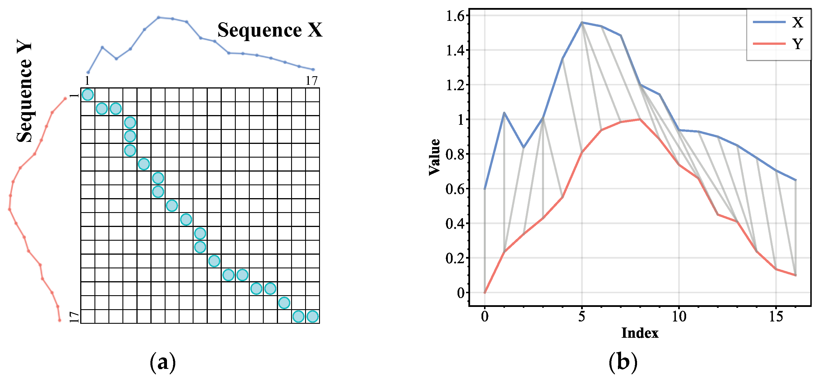
2.3. Dynamic Time Warping

DTW can be used to measure the similarity between two time series [24]. This method aims to find an optimal path by appropriately aligning the data points in the time series to minimize the differences between the two series. We used DTW distance to measure two segments of LIB fluctuation series of the same length. Given two one-dimensional time series of equal length $m$, defined as $X=\{x_1,x_2,\dots ,x_i,\dots ,x_m\}$ and $Y=\{y_1,y_2,\dots ,y_j,\dots ,y_m\}$, where $x_i$ and $y_j$ are the elements of series $X$ and $Y$, respectively.

To calculate the DTW distance between these two series, a distance matrix of size $m\times m$ is first constructed. Each element in the distance matrix is accumulated using the following formula:

$$D\left(i,j\right)=d\left(x_i,y_j\right)+\min \{D\left(i-1,j-1\right),D\left(i-1,j\right),D\left(i,j-1\right)\}$$

(2)

where $d\left(x_i,y_j\right)$ represents the Euclidean distance between $x_i$ and $y_j$.

The value of the top-right element of the matrix, $D\left(m,m\right)$, represents the DTW distance between the two series.

From this point, trace back by selecting the element with the smallest cumulative distance at each step until returning to the starting point $D\left(1,1\right)$. This path represents the optimal path between the two series. The distance matrix $D$, optimal path, and sequence mapping relationship are shown in Figure 2.

2.4. Adaptive Sliding Window–Dynamic Time Warping

The fluctuation series of different LIBs exhibit variations, but after normalization, the key characteristics of each battery’s fluctuation series, such as capacity regeneration and random fluctuations, show similarities [25]. Based on this point, we predicted the capacity fluctuations of the current battery by matching the fluctuation series of other batteries.

The existing LIB data in this paper are referred to as sample data, denoted as $T$. The known sequence to be predicted is referred to as input data, denoted as $P$.

The Fixed-Size Sliding Window–DTW (FSW-DTW) method is shown in Figure 3. First, a sliding window of fixed size $n$ is used to frame the end of the input data, resulting in $P_{sub}=\left(p_1,p_2,\dots ,p_n\right)$. Another window slides over the sample data $T$ to continuously extract subsequences:

$$T_{\mathrm{sub}}\left(i\right)=\left(t_i,t_{i+1},\dots ,t_{i+n-1}\right),\hspace{1em}\mathrm{for}\hspace{1em}i=1,2,\dots ,m-n+1$$

(3)

where $i$ represents the starting position index of the sliding window and $m$ is the total length of the sequence $T$.

$P_{sub}$ is then matched with each subsequence $T_{sub}\left(i\right)$, identifying the segment with the smallest DTW distance, $T_{sub}\left(i*\right)$. The subsequent data point of $T_{sub}\left(i*\right)$, $t_{i*+n}$, is used as the prediction result ${\widehat{p}}_{n+1}$.

$$i*=\underset{i}{\arg \min }\mathrm{DTW}\left(T_{\mathrm{sub}},P_{\mathrm{sub}}\left(i\right)\right),\hspace{1em}\mathrm{for}\hspace{1em}i=1,2,\dots ,m-n+1$$

(4)

$${\widehat{p}}_{n+1}=t_{i*+n}$$

(5)

The FSW-DTW method can predict fluctuation sequences, but its accuracy is limited by the fixed size of the sliding window. This is because a larger sliding window size is more suitable for predicting the flat segments of battery capacity, while a smaller sliding window size offers higher precision in the descending segments following a peak. To address this, in this paper, we introduce a feature recognition-based Adaptive Sliding Window (ASW) strategy to adapt to these varying needs. Figure 4 and Equation (6) illustrate the implementation details of this ASW:

$$W\left(t\right)=\{\begin{array}{cc}1+\frac{1}{\tau }\left(t-t_p\right)& \mathrm{if} t>t_p,\hspace{1em}y\left(t_p\right)-y\left(t_b\right)\ge y_{th},\hspace{1em}1+\left({t-t}_p\right)\le W_0\\ W_0& \mathrm{otherwise}\end{array}$$

(6)

where $W\left(t\right)$ represents the current sliding window size, $W_0$ is the default sliding window size, $t_p$ and $t_b$ represent the cycle periods of the previous peak and trough, respectively, $y_{th}$ is the predetermined rising threshold used to identify rapidly rising segments, and $\tau$ is the window expansion rate coefficient, reflecting the adjustment speed of the window size during rapid rise segments. During prediction, the sliding window size will adaptively adjust according to the characteristics of the feedback LIB SOH series. After encountering a rapid rise peak, the window size will gradually decrease according to the prediction cycle to optimize the prediction of subsequent descending segments. For other parts of the sequence, the default sliding window size $W_0$ is maintained for prediction.

Figure 5 demonstrates the process of predicting fluctuation sequences by utilizing ASW in combination with DTW. The method involves iterating through the sample sequence with a window while employing DTW to identify the optimal matching segment for the current segment of the sequence. The predicted value of the matching segment is then utilized as the prediction outcome for the current segment. This iterative prediction process results in the generation of a continuous predicted fluctuation sequence, thereby establishing a comprehensive prediction sequence.

In this study, we utilize a one-step ahead prediction approach, where the sliding window transitions one step at a time to forecast the upcoming data point’s value:

$${\widehat{p}}_{j+1}=f\left(p_{j-n+1},p_{j-n+2},\dots ,p_j\right),\hspace{1em}j=n,n+1,\dots ,S-1$$

(7)

where j is the end index of the sliding window, n is the window size, and S is the total number of predicted steps.

2.5. Evaluation Metrics

To assess the predictive accuracy of each model, this study employs root mean square error (RMSE) and mean absolute error (MAE) as evaluation measures [26]. RMSE is especially responsive to significant prediction discrepancies, whereas MAE provides a more precise reflection of the true predictive error performance. A lower value for RMSE and MAE signifies the superior predictive capability of the model.

$$RMSE=\sqrt{\frac{1}{n}{\displaystyle \sum _{i=1}^n{\left(y_i-{\widehat{y}}_i\right)}^2}}$$

(8)

$$MAE=\frac{1}{n}{\displaystyle \sum _{i=1}^n}|y_i-{\widehat{y}}_i|$$

(9)

In Equations (8) and (9), $y_i$ represents the actual values of the capacity sequence, while ${\widehat{y}}_i$ represents the predicted values.

3. Experiment

3.1. Dataset

In this study, we conducted an experiment using LIB datasets #5, #6, #7, and #18 obtained from the NASA PCoE Research Center, which represent the degradation data of LIBs numbered B0005, B0006, B0007, and B0018, respectively [11]. Datasets #5, #6, and #18 were employed to generate the sample data, while dataset #7 was set aside as the test dataset. Each dataset involved subjecting LIBs to multiple charge and discharge cycles under consistent temperature (24 °C) settings. The charge and discharge procedures of the LIB during each cycle are depicted in Figure 6.

The charging and discharging process involves three key stages: (1) the constant current charging (CCC) phase where the battery receives a constant current of 1.5 A until the voltage reaches 4.2 V; (2) the constant voltage charging (CV) phase where the battery is charged at a constant voltage until the current decreases to 20 mA; and (3) the constant current discharge (CCD) phase where the battery is discharged at a constant current of 2 A until specific voltage thresholds of 2.7 V, 2.5 V, 2.2 V, and 2.5 V are reached for cells #5, #6, #7, and #18 respectively. The experimental LIB will undergo these aforementioned stages repeatedly until its capacity decreases to 70% of its initial capacity.

3.2. Extraction of Fluctuation Sequences via EMD

According to Equation (1), the capacity sequences in LIB datasets #5, #6, and #18 can be derived by normalizing them to acquire their corresponding SOH sequences. Following EMD decomposition, each SOH sequence is split into a Res sequence and an IMF sequence. The Res sequence captures the primary trend of the battery, depicting the general long-term monotonic trend, while the IMF sequence unveils the local fluctuation properties of battery capacity as a fluctuation sequence. The extraction of fluctuation sequences using the EMD method is depicted in Figure 7.

The leftmost section illustrates three distinct blue sequences denoting the initial State of Health (SOH) sequence, the main trend sequence, and the fluctuation sequence of LIB #5, each comprising 148 elements. In the middle, the orange sequence pertains to LIB #6, consisting of 88 elements. Lastly, on the rightmost side, the green sequence signifies LIB #18, containing 119 elements.

Following the extraction of battery fluctuation sequences IMF5, IMF6, and IMF18 from datasets #5, #6, and #18, respectively, we proceeded to use min–max normalization to generate sample sequences. The fluctuation sequences and sample sequences for each battery can be observed in Figure 8.

3.3. Parameter Determination

Based on Equation (6), the adaptive sliding window strategy proposed in the paper also requires the determination of three parameters: the default sliding window size $W_0$, the window expansion coefficient $\tau$, and the rising threshold $y_{th}$. This section aims to explore the relatively optimal combinations of values to ensure the appropriate setting of these parameters for the subsequent experiments.

3.3.1. Determination of $W_0$

To select the appropriate $W_0$ value, this study employed sliding windows ranging from 1 to 20 using the Fixed-Size Sliding Window–DTW approach to forecast the fluctuation series of LIB #7. The evaluation metrics of the models with varied window sizes, such as RMSE and MAE values, can be observed in Figure 9. Optimal model evaluation metrics are attained when $W_0$ is designated as 3, 7, and 8. Thus, these values are deemed as the most favorable choices for $W_0$. The analysis represented in Figure 9 illustrates that smaller window sizes excel at capturing local patterns of variations while neglecting long-term trends. Conversely, larger window sizes mitigate this drawback but might overlook crucial local traits or introduce excessive noise. This rationale underscores the adoption of ASW.

3.3.2. Determination of $\tau$

In order to establish a suitable $\tau$ value, a constant value of $W_0$ equal to 8 was specified in the paper. Various $\tau$ values ranging from 0.2 to 5 were examined, where each value represents a different window size adjustment rate per cycle period. The ASW-DTW method was employed to examine the predictive performance of the LIB #7 fluctuation sequence across the different $\tau$ values. The analysis depicted in Figure 10 reveals that parameter values of 1 and 5 yield the best RMSE and MAE results. Consequently, these values were deemed optimal and will be further considered in subsequent sections.

3.3.3. Determination of $y_{th}$

In this study, we examined distinct variations between peaks and valleys within a recognized fluctuation sequence, arranging these differences into sequence $\Delta IMF$. To eliminate rapid upward segments in the fluctuation sequence, our analysis assigned the median value of 0.06 from sequence $\Delta IMF$ as the value of $y_{th}$.

3.4. Fluctuation Series Prediction for Capacity

From the findings presented in Section 3.3, six unique combinations of parameter values were derived for the ASW-DTW model: $W_0=3$, $\tau =1$; $W_0=7$, $\tau =1$; $W_0=8$, $\tau =1$; $W_0=3$, $\tau =5$; $W_0=7$, $\tau =5$; $W_0=8$, $\tau =5$. These parameter sets were then applied to predict the fluctuation pattern of LIB #7.

4. Results and Discussion

4.1. Analysis of Results

The prediction results were derived from the experiments conducted. The evaluation metrics for the six ASW-DTW model groups are depicted in

Table 1. Evaluation metrics of ASW-DTW under various parameter combinations.

Index	${\mathit{W}}_0$	$\mathit{\tau }$	RMSE	MAE
1	3	1	9.77%	6.50%
2	7	1	9.71%	6.96%
3	8	1	8.34%	6.33%
4	3	5	10.79%	6.64%
5	7	5	10.16%	6.65%
6	8	5	8.97%	6.11%

.

Figure 11 illustrates the fitted curve showing a comparison between the predicted sequence after inverse normalization and the true values. The orange line depicts the predicted fluctuation sequence, while the blue line represents the actual values.

The experimental findings demonstrate that group 3 and group 6 exhibit the highest accuracy, indicating that a larger sliding window size ($W_0=8$) is advantageous for capturing long-term data trends, making it more suitable for predicting data segments with smoother fluctuations. From Figure 11, it can be seen that the overall fitting degree of the sequences is similar across all groups, and the ability to capture sequence features determines the differences in evaluation metrics among the groups. For rapid declines following peaks, particularly in the 36–40, 57–66, and 143–147 cycles, a quicker window expansion coefficient ($\tau =1$) assists in effectively adjusting the window size to accommodate local data features. However, in the early stages of wave predictions (the first 10 cycles on the graph), group 6 ($\tau =5$) shows superior accuracy due to its slower window expansion rate and consistent size. In contrast, Group 3 shows lower early-stage prediction accuracy, while Group 6 has poorer fitting performance in the steep decline segments. However, both have similar evaluation metrics. Hence, this study will employ the configurations of group 3 and group 6 as the benchmark for evaluating the performance of other prediction methods.

4.2. Comparison with the Other Models

To thoroughly assess the effectiveness of the ASW-DTW model presented in this study, comparative experiments in this section involve two well-established models for fluctuation prediction: the Gaussian Process Regression (GPR) model and the Long Short-Term Memory (LSTM) model. In accordance with Section 3.2, the training datasets for the sample sequences of the ASW-DTW model, LSTM model, and GPR model consist of the fluctuation data of LIB #5, #6, and #18, respectively.

During the experiment, the parameters were established at values where $W_0=8$,$\tau =1$, and $W_0=8$, $\tau =5$. Subsequently, four models were employed to predict the fluctuation sequence of LIB #7. Figure 12 and

Table 2. Evaluation metrics of the different methods.

Index	Method	RMSE	MAE
1	ASW-DTW, $W_0=8$, $\tau =1$	8.34%	6.33%
2	ASW-DTW, $W_0=8$, $\tau =5$	8.97%	6.11%
3	GPR [11]	10.50%	8.74%
4	LSTM [16]	9.87%	8.23%

present the fitting results and predictive evaluation metrics, respectively.

Compared with the GPR and LSTM methods, it is evident from Figure 12 that the two ASW-DTW models exhibit superior performance in forecasting peaks and troughs, as seen in the 8–17, 34–42, and 64–87 cycles. This indicates that the sequence feature capturing ability of GPR and LSTM is weaker than that of the ASW-DTW model, which is better suited for fitting data with significant fluctuations. Compared with the GPR and LSTM methods, it is evident from Figure 12 that of the two ASW-DTW models, Method 1 achieves an RMSE of 8.34%, while Method 2 attains an MAE of 6.11%, both representing optimal results. This underscores the efficacy of the feature recognition-based sliding window adaptive strategy and the predictive accuracy advantage of the ASW-DTW approach.

4.3. Verification of the Generalization Ability of the Model

In order to assess the model’s ability to make general predictions, this study utilized the fluctuation data from LIB #5, #6, and #7 as training data. The ASW-DTW model was applied with parameters $W_0=8$ and $\tau =1$ to forecast the fluctuation data of LIB #18. The prediction outcomes are depicted in Figure 13, with corresponding evaluation metrics detailed in

Table 3. Robustness test evaluation metrics for the different methods.

Index	Method	RMSE	MAE
1	ASW-DTW, $W_0=8$$, \tau =1$	10.97%	6.31%
2	GPR [11]	12.77%	9.59%
3	LSTM [16]	11.17%	9.39%.

. Despite some minor accuracy reductions in specific segments (cycles 15–19 and cycles 47–54), overall model fitting is satisfactory, particularly in recognizing key features of the sequence such as peaks and troughs where the prediction error remains within an acceptable range. Compared with the ASW-DTW method, the GPR model’s fitting curve is too smooth and exhibits underfitting at troughs (cycles 2, 18, 47, and 84). While the LSTM model can capture features, its fitting results fluctuate too wildly, showing overfitting in certain descending segments (cycles 4–15, 50–65, 71–75). The RMSE for the ASW-DTW approach is 10.97%, and that of MAE is 6.31%. In comparison with the GPR and LSTM techniques, this method exhibits superior performance based on the assessment criteria, highlighting its generalizability and resilience.

5. Conclusions

The prediction of LIB capacity fluctuations encounters challenges in capturing local fluctuations accurately, slow computational processes, and significant bias in early predictions. This study introduces a novel approach that integrates ASW and DTW techniques to overcome these obstacles. By utilizing the EMD method to separate main trend sequences from fluctuation sequences, the model can effectively focus on fitting local fluctuations. Additionally, to enhance the model’s transferability and prediction accuracy and reduce DTW computation, a feature recognition-based Adaptive Sliding Window-Assisted DTW prediction method is proposed. Experimental evaluations on diverse LIBs demonstrate that the proposed approach outperforms conventional methods such as GPR and LSTM. This study offers insights into efficiently identifying local battery fluctuations.

In the present study, an exhaustive search method is employed for pattern matching using DTW instead of an optimal matching strategy, leading to a higher computational load. Future investigations could focus on exploring optimal matching strategies to mitigate this issue.

References

1. Wang, Y.; Hei, C.; Liu, H.; Zhang, S.; Wang, J. Prognostics of remaining useful life for lithium-ion batteries based on hybrid approach of linear pattern extraction and nonlinear relationship mining. IEEE Trans. Power Electron. 2022, 38, 1054–1063. [Google Scholar] [CrossRef]
2. Ren, L.; Dong, J.; Wang, X.; Meng, Z.; Zhao, L.; Deen, M. A data-driven auto-CNN-LSTM prediction model for lithium-ion battery remaining useful life. IEEE Trans. Ind. Inform. 2020, 17, 3478–3487. [Google Scholar] [CrossRef]
3. Vermeer, W.; Mouli, G.R.C.; Bauer, P.J.I.T.o.T.E. A comprehensive review on the characteristics and modeling of lithium-ion battery aging. IEEE Trans. Transp. Electrif. 2021, 8, 2205–2232. [Google Scholar] [CrossRef]
4. Xu, K.; Yang, H.; Zhu, C.; Jin, X.; Fan, B.; Hu, L. Deep extreme learning machines based two-phase spatiotemporal modeling for distributed parameter systems. IEEE Trans. Ind. Inform. 2022, 19, 2919–2929. [Google Scholar] [CrossRef]
5. Wang, Z.; Liu, N.; Chen, C.; Guo, Y.J.I.S. Adaptive self-attention LSTM for RUL prediction of lithium-ion batteries. Inf. Sci. 2023, 635, 398–413. [Google Scholar] [CrossRef]
6. Huang, Y.; Zhang, P.; Lu, J.; Xiong, R.; Cai, Z. A transferable long-term lithium-ion battery aging trajectory prediction model considering internal resistance and capacity regeneration phenomenon. Appl. Energy 2024, 360, 122825. [Google Scholar] [CrossRef]
7. Ma, G.; Zhang, Y.; Cheng, C.; Zhou, B.; Hu, P.; Yuan, Y. Remaining useful life prediction of lithium-ion batteries based on false nearest neighbors and a hybrid neural network. Appl. Energy 2019, 253, 113626. [Google Scholar] [CrossRef]
8. He, N.; Yang, Z.; Qian, C.; Li, R.; Gao, F.; Cheng, F. Remaining useful life prediction of lithium-ion battery based on fusion model considering capacity regeneration phenomenon. J. Energy Storage 2024, 85, 111068. [Google Scholar] [CrossRef]
9. Cui, Y.; Chen, Y. Prognostics of lithium-ion batteries based on capacity regeneration analysis and long short-term memory network. IEEE Trans. Instrum. Meas. 2022, 71, 1–13. [Google Scholar] [CrossRef]
10. Han, J.; van der Baan, M. Empirical mode decomposition for seismic time-frequency analysis. Geophysics 2013, 78, O9–O19. [Google Scholar] [CrossRef]
11. Liu, K.; Shang, Y.; Ouyang, Q.; Widanage, W.D. A data-driven approach with uncertainty quantification for predicting future capacities and remaining useful life of lithium-ion battery. IEEE Trans. Ind. Electron. 2020, 68, 3170–3180. [Google Scholar] [CrossRef]
12. Cheng, G.; Wang, X.; He, Y. Remaining useful life and state of health prediction for lithium batteries based on empirical mode decomposition and a long and short memory neural network. Energy 2021, 232, 121022. [Google Scholar] [CrossRef]
13. Wei, M.; Ye, M.; Zhang, C.; Li, Y.; Zhang, J.; Wang, Q. A multi-scale learning approach for remaining useful life prediction of lithium-ion batteries based on variational mode decomposition and Monte Carlo sampling. Energy 2023, 283, 129086. [Google Scholar] [CrossRef]
14. Wang, S.; Ma, H.; Zhang, Y.; Li, S.; He, W. Remaining useful life prediction method of lithium-ion batteries is based on variational modal decomposition and deep learning integrated approach. Energy 2023, 282, 128984. [Google Scholar] [CrossRef]
15. Liu, K.; Tang, X.; Teodorescu, R.; Gao, F.; Meng, J. Future ageing trajectory prediction for lithium-ion battery considering the knee point effect. IEEE Trans. Energy Convers. 2021, 37, 1282–1291. [Google Scholar] [CrossRef]
16. Wang, J.; Zhang, S.; Li, C.; Wu, L.; Wang, Y.J. A data-driven method with mode decomposition mechanism for remaining useful life prediction of lithium-ion batteries. IEEE Trans. Power Electron. 2022, 37, 13684–13695. [Google Scholar] [CrossRef]
17. Fu, J.; Wu, C.; Wang, J.; Haque, M.M.; Geng, L.; Meng, J. Lithium-ion battery SOH prediction based on VMD-PE and improved DBO optimized temporal convolutional network model. J. Energy Storage 2024, 87, 111392. [Google Scholar] [CrossRef]
18. Luo, K.; Chen, X.; Zheng, H.; Shi, Z. A review of deep learning approach to predicting the state of health and state of charge of lithium-ion batteries. J. Energy Chem. 2022, 74, 159–173. [Google Scholar] [CrossRef]
19. Sun, H.; Yang, D.; Wang, L.; Wang, K. A method for estimating the aging state of lithium-ion batteries based on a multi-linear integrated model. Int. J. Energy Res. 2022, 46, 24091–24104. [Google Scholar] [CrossRef]
20. Kim, H.; Ahn, C.R.; Engelhaupt, D.; Lee, S. Application of dynamic time warping to the recognition of mixed equipment activities in cycle time measurement. Autom. Constr. 2018, 87, 225–234. [Google Scholar] [CrossRef]
21. Jorge, I.; Mesbahi, T.; Samet, A.; Boné, R. Time series feature extraction for lithium-ion batteries state-of-health prediction. J. Energy Storage 2023, 59, 106436. [Google Scholar] [CrossRef]
22. Wang, Z.; Liu, N.; Guo, Y. Adaptive sliding window LSTM NN based RUL prediction for lithium-ion batteries integrating LTSA feature reconstruction. Neurocomputing 2021, 466, 178–189. [Google Scholar] [CrossRef]
23. Zhang, X.; Xiang, H.; Xiong, X.; Wang, Y.; Chen, Z. Benchmarking core temperature forecasting for lithium-ion battery using typical recurrent neural networks. Appl. Therm. Eng. 2024, 248, 123257. [Google Scholar] [CrossRef]
24. Li, H. Time works well: Dynamic time warping based on time weighting for time series data mining. Inf. Sci. 2021, 547, 592–608. [Google Scholar] [CrossRef]
25. Dunn, J.; Huang, C.-S. A P-Value Approach for Real-Time Identifying the Capacity Regeneration Phenomenon of Lithium-ion Batteries. In Proceedings of the 2023 IEEE 3rd International Conference on Industrial Electronics for Sustainable Energy Systems (IESES), Shanghai, China, 26–28 July 2023; pp. 1–6. [Google Scholar]
26. Zhou, D.; Li, Z.; Zhu, J.; Zhang, H.; Hou, L. State of health monitoring and remaining useful life prediction of lithium-ion batteries based on temporal convolutional network. IEEE Access 2020, 8, 53307–53320. [Google Scholar] [CrossRef]
Figure 1. Proposed method.
Electronics 13 02501 g001
Figure 2. The DTW process: (a) optimal path and (b) sequence mapping relationship.
Electronics 13 02501 g002
Figure 3. The process of FSW-DTW.
Electronics 13 02501 g003
Figure 4. Sliding window adaptive strategy.
Electronics 13 02501 g004
Figure 5. ASW-DTW prediction process.
Electronics 13 02501 g005
Figure 6. Charging and discharging process of LIBs.
Electronics 13 02501 g006
Figure 7. Extraction of fluctuation sequences.
Electronics 13 02501 g007
Figure 8. Results of fluctuation sequences extraction: (a) IMF5; (b) IMF6; (c) IMF18; (d) empirical sequence.
Electronics 13 02501 g008
Figure 9. Comparison of RMSE and MAE values for different sizes of sliding windows.
Electronics 13 02501 g009
Figure 10. Comparison of RMSE and MAE values for different window expansion rate coefficient.
Electronics 13 02501 g010
Figure 11. Prediction results for LIB #7 using ASW-DTW with selected optimal parameter combinations: (a) W 0 = 3 , τ = 1 ; (b) W 0 = 7 , τ = 1 ; (c) W 0 = 8 , τ = 1 ; (d) W 0 = 3 , τ = 5 ; (e) W 0 = 7 , τ = 5 ; (f) W 0 = 8 , τ = 5 .
Electronics 13 02501 g011
Figure 12. Comparison of the experimental results with the other methods: (a) ASW-DTW, W 0 = 8 , τ = 1 ; (b) ASW-DTW, W 0 = 8 , τ = 5 ; (c) GRP; (d) LSTM.
Electronics 13 02501 g012
Figure 13. Prediction results for LIB #18: (a) ASW-DTW, W 0 = 8 , τ = 1 ; (b) GPR; (c) LSTM.
Electronics 13 02501 g013