All articles published by MDPI are made immediately available worldwide under an open access license. No special
permission is required to reuse all or part of the article published by MDPI, including figures and tables. For
articles published under an open access Creative Common CC BY license, any part of the article may be reused without
permission provided that the original article is clearly cited. For more information, please refer to
https://www.mdpi.com/openaccess.
Feature papers represent the most advanced research with significant potential for high impact in the field. A Feature
Paper should be a substantial original Article that involves several techniques or approaches, provides an outlook for
future research directions and describes possible research applications.
Feature papers are submitted upon individual invitation or recommendation by the scientific editors and must receive
positive feedback from the reviewers.
Editor’s Choice articles are based on recommendations by the scientific editors of MDPI journals from around the world.
Editors select a small number of articles recently published in the journal that they believe will be particularly
interesting to readers, or important in the respective research area. The aim is to provide a snapshot of some of the
most exciting work published in the various research areas of the journal.
As more and more new power electronics with high switching frequencies are used in power-electronic equipment on ships and other platforms, the wideband radiation that power-electronic equipment gives off could affect sensitive equipment on the platform. Therefore, it is crucial to accurately model and characterize its wideband radiation properties to predict the wideband field distribution near such equipment. The traditional equivalent dipole method is commonly used to model power-electronic equipment at a single frequency. It is difficult to apply this method to wideband applications, and the precision of equivalent dipole array modeling at each frequency is insufficient. Additionally, acquiring the near-field phase data necessary for comparable modeling through practical measurement is frequently difficult. To solve the above problems, this paper proposes an equivalent dipole hybrid modeling method for power-electronic equipment’s broadband radiation characteristics. Starting with the near-field data at finite frequency points in a wideband, the method employs a global optimization algorithm to find the best equivalent dipole array, which characterizes the power-electronic equipment’s radiation characteristics. Furthermore, the interpolation technique is used to predict the wideband radiation properties of power-electronic equipment. Finally, test and numerical examples demonstrate the method’s accuracy and effectiveness.
With the wide application of high-switching frequency and high-power semiconductor devices in the power-electronic equipment of ships and other platforms, the electromagnetic radiation produced by the power-electronic equipment is increasing, and the coverage frequency band is expanding. Furthermore, when the magnetic radiation interference from power-electronic equipment on ships exceeds the electromagnetic susceptibility (EMS) threshold of sensitive devices such as low-frequency communication, navigation, and detection equipment, it may degrade performance or disrupt their normal operation due to their limited immunity [1,2,3]. EMS refers to the ability of power-electronic equipment to resist external electromagnetic interference, while radiation is the source of electromagnetic interference. To conduct more accurate and comprehensive electromagnetic compatibility (EMC) analysis, it is urgent to accurately model and characterize the broadband radiation characteristics of power-electronic equipment. This will make it possible to quantitatively predict the broadband field distribution characteristics of the s power-electronic equipment, support the control of broadband radiation electromagnetic interference, and improve the EMC performance of the entire platform [4,5]. Currently, the modeling methods for the broadband radiation characteristics of power-electronic equipment are primarily divided into two groups. One is the full-wave modeling method [6,7], which needs to accurately grasp the electromagnetic parameters, circuit topology, specific structure, current path, and other detailed information of the radiation source to establish the radiation characteristics model of complex power-electronic equipment. In fact, it is very difficult to obtain all the necessary information for full-wave modeling of complex power-electronic devices in the EMC design of platforms such as ships.
On the other hand, researchers have also proposed some equivalent source modeling methods for characterizing the radiation properties of power-electronic devices. These methods are based on the Huygens principle and near-field data to establish an equivalent model of radiation sources. They include the mode expansion method [8], the integral equation method [9], the equivalent electromagnetic current method [10], and the equivalent dipole method [11,12,13,14]. Table 1 details the merits and limitations of various equivalent source modeling approaches. The equivalent dipole method is the simplest, and Hertzian dipoles, with their analytical radiation formula and ease of analysis, represent the most widely used modeling method. It obtains the near-field data of the power-electronic device by measurements or other means and then solves a set of linear equations to create an equivalent dipole array model of the radiation source. Once the equivalent dipole array model of the real radiation source is found, full-wave analysis software can be used to predict the radiation field distribution near power-electronic devices on the equipment platform.
Equivalent dipole modeling is classified into two types based on the computational domain: time-domain equivalent dipole modeling and frequency-domain equivalent dipole modeling. The time-domain equivalent dipole model can be utilized to model a wideband radiation source. Reference [15] proposes a theoretical analysis method that overlooks the delay time between dipole sources, making it difficult to accurately calculate the field distribution near the radiation source. Reference [16] introduces an improved modeling method that uses tangential magnetic field components acquired at different points in time from near-field scanning, reducing the number of dipole arrays and improving calculation speed. Reference [17] considers the delay time in the time domain and develops a time-dependent dipole array model using measured magnetic fields to characterize the object. Although the time-domain dipole equivalent modeling method is theoretically suitable for wideband modeling, its accuracy is low and depends on the accuracy and dynamic range of the time-domain near-field scanning data. Meanwhile, issues such as the narrow dynamic range of time-domain testing technology make it difficult to further improve its modeling accuracy, and it fails to meet the requirements for high-precision modeling and prediction in real engineering.
On the other hand, the frequency-domain equivalent dipole modeling method is more accurate and applicable. At present, the modeling methods for broadband radiation sources using equivalent dipoles include the rational function modeling method [18], the modeling method based on “hotspot” data [19], the neural network method [20], the interpolation method [21,22], etc. The rational function modeling method [23] uses a single rational function to characterize the wideband equivalent source model and obtains the coefficients of the rational function by solving linear equations. The modeling method based on “hotspot” data [19] is to establish an equivalent dipole array model using the maximum near-field radiation test data at each frequency point within a wide frequency band. The neural network modeling method [20] uses the parallel operation of Green’s function at a few frequency points as the input for the neural network training set and the parallel operation of near-field amplitude at multiple frequency points as the output for the neural network training set. By utilizing the powerful self-learning and non-linear mapping capabilities of artificial neural networks, a well-trained neural network can predict the amplitude and phase information of the wideband radiation field within a certain error range. However, to obtain accurate prediction results, this method requires enough training data and an appropriate neural network structure for optimal training. This requires measuring the near-field data of many near-field planes at various heights, as well as a significant amount of computing resources to support the training process. The idea of employing the interpolation technique [21,22] to achieve equivalent modeling of a wideband radiation source is to infer the dipole array model of other frequency points based on the known dipole array model at specific frequency points. Since this method largely depends on the fitting of the data of known frequency points, a wideband radiation source reconstruction method based on numerical Green’s function and cubic spline interpolation is proposed in [21], and an adaptive frequency sampling method is proposed to determine the interpolation frequency. T. Song also proposes a modeling method for a wideband radiation source using near-field data without phase information [22]. This method first scans the near-field radiation amplitude data at three predetermined frequencies, then uses the differential evolution (DE) algorithm to obtain the dipole array, and finally uses the interpolation algorithm to obtain the wideband equivalent array model. However, the initial value setting of the DE algorithm greatly affects the speed and results of optimization. Furthermore, to aid interpolation, the position and number of magnetic dipoles are maintained constant at each frequency. Although the method is simple and straightforward, the accuracy of the equivalent model suffers when the extrapolation frequency deviates significantly from the minimum or maximum frequency of the preset measured frequency.
In real engineering, accurate acquisition of near-field phase information requires reference probes or reference signals, which complicates measurements and makes it time-consuming. If the near-field distribution data on the plane lacks phase information, the modeling speed of the near-field test data will be significantly accelerated. However, the establishment of the equivalent dipole array model then becomes an optimal solution problem. Current solutions include global optimization algorithms [23,24], phase recovery algorithms [25], and neural networks [26,27]. Global optimization algorithms, such as particle swarm optimization (PSO) and DE, can be utilized for the equivalent dipole modeling of near-field data without phase information. However, the drawback of such a method is that the computational efficiency decreases sharply as the number of dipoles increases. The initial value of the algorithm also affects its efficiency and accuracy. The phase recovery algorithm requires near-field data of the measured plane at two different heights, thus resulting in a long scanning time. To overcome these problems, Y. F. Shu proposes a single-sided iterative reconstruction algorithm to decrease the scanning time [25]. X. C. Wei established a new mapping relationship between dipole arrays and radiation fields using the equivalent dipole model and an artificial neural network (ANN) [26]. J. Wen introduces a cascade forward neural network (CFNN) to establish a nonlinear relationship between Green’s function and the radiation field intensity [27].
There are still some challenges in modeling the equivalent dipole array for wideband radiation sources, such as inaccuracies and the lack of a unified modeling method based on near-field with phase or phase-free data. To address these challenges, an equivalent dipoles modeling hybrid method that combines the adaptive differential evolution (ADE) algorithm with an optional external archive with an interpolation algorithm is proposed in this paper for modeling the wideband radiation characteristics of power-electronic devices. In this method, the optimal magnetic dipole array is determined using the global optimization capability of the ADE algorithm, which is applied to near-field data with or without phase information. First, high-precision equivalent modeling is achieved at n preset test frequency points, and then the interpolation method is used to obtain the corresponding dipole arrays at other extrapolated frequency points. The unified equivalent dipole array modeling method for wideband radiation, based on near-field with phase or phase-free data, has been developed.
The rest of this paper is organized as follows: First, Section 2 describes a hybrid method for modeling the wideband radiation characteristics of power-electronic equipment. In Section 3, some examples are used to validate the feasibility and effectiveness of the proposed hybrid modeling method, and the modeling effect of the wideband modeling method is also discussed. Some conclusions are drawn in Section 4.
2. Description of the Hybrid Modeling Method
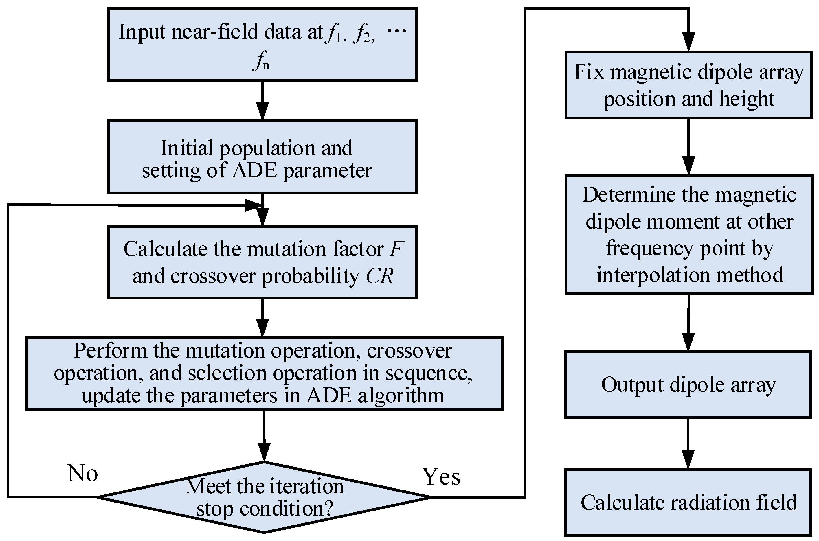
To improve the accuracy of equivalent modeling for wideband radiation sources of power-electronic equipment and deal with the challenge of unified modeling using near-field data, whether phase information is available, this paper proposes an equivalent dipole modeling method for wideband radiation characteristics of power-electronic equipment by combing the ADE algorithm with an interpolation algorithm. The modeling idea is as follows: Based on the near-field radiation characteristic test data at finite frequency points near the power-electronic equipment, a global optimization algorithm is used to determine the optimal equivalent dipole array that characterizes the wideband radiation characteristic of the power-electronic equipment. Then, the wideband radiation characteristics of power-electronic equipment are predicted using the interpolation technique. Finally, some examples are provided to demonstrate the accuracy and availability of the method. The specific process is shown in Figure 1.
The detailed steps of the hybrid modeling method are as follows:
Step 1: The near-field radiation data of the equipment at preset frequency test points within a wideband is obtained through near-field measurements. This section takes n preset frequency points as an example to discuss the wideband radiation equivalent modeling method. The frequency values are chosen randomly. These frequency points are as follows: , and .
Step 2: Based on the available near-field data, an optimal equivalent dipole array model at n frequency points is established using the global optimization capability of the ADE algorithm. As a result, high-precision equivalent modeling is realized at n frequency points.
(1)
If the field distribution data in the near-field plane includes phase information, there is a clear relationship between the array model and the data. The equivalent dipole array radiation model can be solved by setting the dipole coordinates. However, the efficiency and accuracy of equivalent modeling are constrained by the height of the array, as well as the number and distribution of dipoles. To further enhance the accuracy of equivalent modeling and address the selection problem of the number and distribution of dipoles and the height of the array, this paper utilizes the ADE algorithm to optimize the dipole array model. When the ADE algorithm is used on the equivalent dipole array modeling based on near-field data with phase information, specific steps and processes are mentioned [28].
(2)
If the field distribution data in the near-field plane lacks phase information, developing an equivalent dipole array model becomes an optimal solution to the nonlinear problem. In this case, the ADE algorithm is used to solve the equivalent dipole array model.
When applying the ADE algorithm and near-field data without phase information to model wideband radiation, it is necessary to initialize the population and set the optimization parameters. The ADE algorithm requires optimization parameters to be set, , , , and , and the specific processes and steps are referenced [29]. The individual’s expression within the population is shown in the following equation:
where o is the serial number of the magnetic dipole, , and m is the total number of magnetic dipoles; xo and yo are the coordinate components of the o-th magnetic dipole; , , and are the components of the dipole moment of the o-th magnetic dipole at a frequency of , respectively. h is the height of the magnetic dipole array. Re( ) and Im( ) are the real and imaginary parts of the magnetic dipole moment, respectively.
The basic principle of ADE is consistent with the classical differential evolution algorithm. Through mutation, crossover, and selection operations, the optimal solution is found through iterative processes. The two control parameters of the classical differential evolution algorithm, the crossover probability factor, CR, and the scaling factor, F, are determined based on the specific optimization problem. The ADE algorithm introduces an external storable population, denoted as A, and a new mutation strategy. It can also adaptively update the algorithm parameters, eliminating the need for constant testing to determine the optimal control parameter values. The algorithm has improved its convergence speed, global optimization capability, and ability to solve high-dimensional problems.
Next, we must define the fitness function in the ADE algorithm, which directs the population’s evolution toward error reduction. As a result, the fitness function is represented by the relative error [17,21], as given in Equation (2). Following that, each iteration can result in an optimal dipole array by performing mutation, crossover, and selection operations. This indicates that the modeling accuracy is greater than a predetermined value at n frequency test points.
where n is the number of frequency points. N is the total number of points in the near-field plane at each frequency point. t takes the x, y, and z components; w refers to the serial number of the calculated frequency point; q refers to the serial number of the measurement point on the near-field plane at each frequency point; is the value of the t-component magnetic field on the q-th measurement point at the w-th frequency point; is the calculated value of the t-component magnetic field on the q-th measurement point at the w-th frequency point. a and b are control variables. When the modeling method is based on near-field data with phase information, a and b take the values 1 and 0, respectively; otherwise, 0 and 1 are used. When phase information is available in the near-field data, the error is defined as the difference between the measured magnetic field and the magnetic field generated by the equivalent magnetic dipoles. When phase information is unavailable, the error function is defined as the difference between the measured magnetic field amplitude and the magnetic field generated by the equivalent magnetic dipole array.
From the perspective of equivalent modeling of wideband radiation sources based on the above two types of near-field data, the process remains the same. The distinction lies in the setting of the population individual and the fitness function of the ADE algorithm during the modeling process. The population setting of wideband radiation equivalent modeling with phase information in near-field radiation data is determined by the position and number of dipoles. The population setting of the wideband radiation equivalent model without phase information is determined by the position of the dipole and the moment component of the magnetic dipole corresponding to each frequency point.
Step 3: Based on the known optimal magnetic dipole array model at n frequency test points, the magnetic dipole moment of the array is determined using the equivalent dipole method. The magnetic dipole moment at other calculated frequency points is then calculated using the interpolation method.
The radiation interference at each frequency within a frequency band of power-electronic equipment is produced by the same circuit topology and physical structure. This implies that the radiation properties of the radiation source at various frequency points in the wideband are inherently linked. Dipole arrays at different frequency points can be obtained using the interpolation method, as demonstrated in the following equation.
where o is the serial number of the magnetic dipole, , and m is the total number of magnetic dipoles; t is the x, y, and z components; is the w-th calculated frequency point in the broadband or outside the frequency band; is the moment of o-th magnetic dipole at a frequency of . Interp( ) represents interpolation techniques, including linear interpolation, cubic interpolation, spline interpolation, Lagrange’s interpolation, etc. These techniques can determine the dipole moment at based on the dipole moments at . a and b are control variables. When the modeling method is based on near-field data with phase information, a and b take the values 1 and 0, respectively; otherwise, 0 and 1 are used.
Step 4: Finally, after the magnetic dipole moments at the calculated frequency point are obtained, the wideband radiation characteristics of power-electronic equipment can be accurately and effectively characterized, based on the relationship between the magnetic dipoles’ moments and the radiation field at any observation point.
where , , and are the magnetic dipole moments in the x, y, and z directions of the j′-th magnetic dipole in the i′-th dipole plane, respectively; where , where is the number of dipole planes; , where is the number of magnetic dipoles in each dipole plane. , , are the x, y and z components of the magnetic field at the j-th measuring point in the i-th near-field plane, , ; is the number of tests in each measured plane.
, , and are shown in Equation (5).
where , , and are the x, y, and z coordinates of the j-th measuring point in the the i-th near-field plane, respectively; , , and are the x, y, and z coordinates of the j′-th magnetic dipole in the i′-th dipole plane, respectively.
is the wave number in free space and is the distance between the magnetic dipole and any observation point. , , and are given in Equation (6).
3. Experiment and Simulation Verification
In this section, a model for wideband radiation interference of power-electronic equipment is developed to validate the accuracy of the proposed method, and the model is validated using experiments and full-wave simulation. Section 3.1 presents an experiment to verify the hybrid modeling method. Section 3.2 verifies the effectiveness of the hybrid modeling method using near-field data with phase-free information, and Section 3.3 provides verification for the hybrid modeling method using near-field data with phase information.
3.1. Experiment Verification
To validate the hybrid modeling method developed in this paper, experiments are first carried out to simulate the radiation interference produced by power-electronic equipment. The signal source generates a sinusoidal signal with a peak-to-peak amplitude of 2 V that is then routed to a frequency characteristic module. The device is connected to a low-frequency loop antenna in an aluminum shell, which generates low-frequency radiation by producing a specific current intensity. The aluminum enclosure’s back is wired to external devices, and all holes and gaps are filled with shielding tape. Low-frequency near-field data is collected around the radiation source using a three-axial fluxgate and a magnetic effect measurement system. Figure 2 displays the test situation [28].
The near-field data surrounding the radiation source is measured using flux gates and grid magnetic measuring equipment. The measuring plane is positioned at a distance of 12.5 cm from the object being measured, and it has dimensions of 85 cm × 100 cm. The length of the object varies from −35 cm to 50 cm, while its width extends from −50 cm to 50 cm. The measurement sites are evenly distributed at intervals of 5 cm, giving a total of 378 measurement points.
The magnetic field distribution at a distance of 12.5 cm, recorded at a frequency of 60 Hz, is depicted in Figure 3.
In our validation example, the radiation characteristics at a frequency of 60 Hz for the measured object are modeled using an equivalent array of 36 magnetic dipoles. In the ADE algorithm, the iteration process is terminated when the population optimal fitness value is less than 0.22. The corresponding magnetic dipole array model can be solved by the hybrid modeling method, and then the predicted magnetic field distributions at 12.5 cm using the equivalent dipole array model are plotted in Figure 4.
The relative error of magnetic field amplitude obtained by the hybrid modeling method is calculated by Equation (2), and the results are given in Table 2. For ease of comparison, the error of the decimal representation is converted to dB, preserving multiple decimal points.
The comparison of Figure 3 and Figure 4 reveals that the magnetic field distribution derived by the proposed hybrid technique closely matches the test ones. Table 2 shows that the relative error between the measured value and the calculated value is typically less than 1.7 dB. Errors arise from the measurement process, such as imprecise positioning of the vector fluxgate on the test plane, environmental noise [11], and calibration errors of the vector fluxgate sensor [17]. Additionally, due to a trade-off between accuracy and computational resources [30], the preset fitness value does not reach its theoretical minimum of 0, implying that the obtained equivalent dipole model may not be unique.
3.2. Modeling Verification of Wideband Radiation Interference in an Electronic Cabinet without Near-Field Phase Information
To validate the equivalent dipole array hybrid modeling method for using near-field with phase-free data to predict wideband radiation characteristics of power-electronic equipment based on the ADE algorithm and interpolation method, the wideband radiation characteristics of a power-electronic cabinet are analyzed, and the corresponding numerical simulation model is established using the full-wave simulation software Ansys 2023 R2 Maxwell 3D, as shown in Figure 5. The solver mode is “Eddy Current”. The cabinet material is defined as iron, and the coil is copper material. The exterior surface of the air box is set as “Radiation Boundary”. Adaptive meshing is employed to refine the mesh. Solver conditions are specified, with the maximum convergence steps set to 10 and the convergence percentage error limited to 1%, while other parameters remain at default settings.
The size of the cabinet model is set to be 1.70 m × 1.10 m × 2.4 m, and it consists of three small cabinets. Each cabinet contains a coil arranged as a simulated radiation source, with currents of kA, kA, and kA, respectively.
3.2.1. Verification of the Hybrid Modeling Method
The wideband radiation equivalent model of the device is established using near-field data with no phase information. In this case, a planar magnetic dipole array with 16 magnetic dipoles is created. The dimensions of the measurement plane, magnetic dipole array plane, and extrapolation plane are 2.8 m × 2.8 m, located 0.1 m, 0.05 m, and 0.4 m away from the cabinet, respectively. The length ranges from −140 cm to 140 cm, and the width ranges from −140 cm to 140 cm. The measurement interval is 10 cm, with 841 points measured. The magnetic field distribution at measured frequency points (60 Hz, 180 Hz, 210 Hz, and 240 Hz) is obtained through Maxwell 3D simulation. Next, set the parameters according to the ADE optimization algorithm: p = 0.2, μCR = 0.5, μF = 0.5, and c = 0.1.
Using 120 Hz and 360 Hz as calculated examples, one frequency point is within the test frequency band, while the other is outside of it. The magnetic dipole arrays corresponding to the above two calculated frequency points are obtained by the proposed modeling method. To avoid too many field graphs, taking the distribution of the calculated plane magnetic field at 120 Hz as an example, the simulated magnetic field distribution of the plane at 120 Hz is shown in Figure 6.
The iteration process ends when the optimal fitness value of the population is less than 0.10. The predicted magnetic field distribution at 120 Hz on the calculation plane by the magnetic dipole array model is shown in Figure 7.
By comparing Figure 6 and Figure 7, it is clear that the predicted magnetic field distribution at 120 Hz, with the modeling method agrees well with the results obtained by Maxwell 3D.
To further quantify the accuracy of the proposed hybrid modeling method, the relative error of the amplitude of each magnetic field component obtained by the proposed method is calculated using equation (2), and the results are listed in Table 3.
As shown in Table 3, the wideband radiation equivalent modeling method, based on the ADE algorithm and interpolation method, produces small relative errors for each magnetic field component, with no more than 1.1 dB at 120 Hz and no more than 2.1 dB at 360 Hz. This indicates that the method can achieve an equivalent model with high accuracy. Furthermore, the magnetic dipole equivalent array model shows higher accuracy when the calculated frequency falls within the predefined measured frequency band.
3.2.2. Analysis of the Interpolation Method’s Effect on Modeling Accuracy
We further explore the impact of the interpolation strategy on the modeling accuracy of wideband radiation characteristics. After determining the optimum group, linear interpolation [31], spline interpolation [32], and the piecewise cubic Hermite interpolation polynomial (PCHIP) method [33] are used to obtain the corresponding equivalent dipole array, and the radiations at 150 Hz, 200 Hz are then calculated. The relative errors of the magnetic dipole array equivalent model at 120 Hz and 360 Hz are calculated by Equation (2), and the results are shown in Table 4.
It can be seen that using the piecewise cubic Hermite interpolation polynomial, the radiation at 150 Hz has a lower magnetic field amplitude error. Compared to the linear interpolation method, the piecewise cubic Hermite interpolation polynomial reduces the amplitude error by 2.4126 dB. Furthermore, compared to spline interpolation, the piecewise cubic Hermite interpolation polynomial reduces the amplitude error by 1.5651 dB. On the other hand, spline interpolation achieves a smaller radiation amplitude error at 200 Hz. In contrast to the linear interpolation strategy, spline interpolation reduces the amplitude error by 2.1491 dB. Compared to piecewise cubic Hermite interpolation polynomials, spline interpolation reduces the amplitude error by 1.3225 dB. These results represent improvements over the linear interpolation method.
3.3. Modeling Verification and Analysis of Cabinet Wideband Radiation Interference with Near-Field Phase Information
In this section, we further validate the proposed equivalent dipole array hybrid modeling method for the wideband radiation characteristics of power-electronic equipment using near-field data with phase information. The wideband radiation characteristics of a power-electronic cabinet are investigated, and the related 3D electromagnetic model is created in the Maxwell 3D software, as shown in Figure 8.
The dimensions of the power-electronic device cabinet are set to be 2.26 m × 1.10 m × 2.24 m. The cabinet consists of four small cabinets with a coil to simulate radiation sources. The alternating current flowing through the coil is kA.
3.3.1. Verification of the Hybrid Modeling Method
An array of 16 magnetic dipoles is used to model the radiation characteristics of the electronic cabinet. First, the Maxwell 3D software is used to obtain magnetic field data with phase information at three frequency test points: 60 Hz, 180 Hz, and 240 Hz. The parameters of the ADE optimization algorithm are set as follows: p = 0.2, μCR = 0.5, μF = 0.5, and c = 0.1. The population individual is set as a row vector with 9 entries, as shown in the following equation.
where o is the serial number of the magnetic dipole, with o ranging from 1 to 16. , , , , , and represent the x and y coordinates of magnetic dipoles in regions A, B, and C [28]. and represent the number of magnetic dipoles in regions A and B, respectively. h represents the height of the array.
Next, according to the fitness function in Equation (2), the iteration process in our simulation will stop when the population optimal fitness value is less than 0.10. At this point, the optimal population can be determined. The output includes the coordinates of the magnetic dipole array, as well as the height of the dipole array and the number of dipoles in various regions.
Subsequently, the magnetic dipole array corresponding to the two calculated frequencies of 120 Hz and 360 Hz can be calculated. To avoid too many field graphs, taking the distribution of the calculated plane magnetic field at 120 Hz as an example, the simulated magnetic field distribution of the plane at 120 Hz is shown in Figure 9.
The components of magnetic dipole moments at 120 Hz and 360 Hz, obtained through the interpolation method, are shown in Figure 10. It is clear that the variation trend of each magnetic dipole moment component at different frequencies is nearly identical. This means that the magnetic dipole moments acquired from near-field data of the same radiation source at different frequencies are interrelated and that the magnetic dipole moments of the same array at different frequencies follow similar distribution patterns.
The predicted magnetic field distributions at 120 Hz on the calculating plane using the equivalent dipole array model are plotted in Figure 11.
The comparison between Figure 9 and Figure 11 indicates that the magnetic field distribution at 120 Hz obtained by this method is nearly the same as the simulated ones.
The relative errors of the magnetic dipole array equivalent model at 120 Hz and 360 Hz are calculated using Equation (2), and the results are shown in Table 5.
Table 5 shows that the modeling method achieves high accuracy in the studied frequency with small relative errors for each magnetic field component. In addition, the equivalent modeling method achieves greater accuracy in the magnetic dipole array modeling at frequency points within the measured frequency band. However, errors in equivalent modeling will increase for frequency points beyond the measured frequency range.
To further validate the proposed hybrid modeling method, a 10-m measurement line is selected. It is perpendicular to the side edge of the equipment and forms a 45-degree angle with the positive z-axis. Observation points are obtained at 0.25-m intervals along this line. The accurate value obtained from the full-wave simulation (Maxwell3D) is compared with the calculated value obtained from the wideband magnetic dipole array model, as shown in Figure 12.
The relative errors between the accurate values at each test point on the measurement line and the calculated values obtained by the wideband equivalent model are all less than 0.95 dB. Thus, the wideband equivalent modeling method proposed in this paper can also ensure precise predictions in long-distance tests.
3.3.2. Analysis of Factors Influencing Wideband Modeling Accuracy
To gain a better understanding of the accuracy and effectiveness of the wideband radiation modeling method, we use an electronic cabinet in Section 3.3 as a case study. We chose the 8 kHz to 2048 kHz frequency range for wideband equivalent modeling. Near-field data are collected at frequency points of 8 kHz, 16 kHz, 32 kHz, 64 kHz, 128 kHz, 256 kHz, 512 kHz, 1024 kHz, and 2048 kHz, with each subsequent frequency point being twice the previous one.
First, frequency points for wideband modeling are selected at one-point intervals inside the 8 kHz to 2048 kHz range, including 8 kHz, 32 kHz, 128 kHz, 512 kHz, and 2048 kHz. The wideband radiation equivalent model is built based on the near-field data at these frequency points. Table 6 presents the relative errors of the calculated magnetic field amplitudes on the plane at 16 kHz, 64 kHz, 256 kHz, and 1024 kHz.
Secondly, we develop a wideband radiation model using near-field data gathered at 8 kHz, 32 kHz, 128 kHz, and 512 kHz. Table 7 shows the relative errors of the calculated magnetic field amplitudes on the plane at 16 kHz, 64 kHz, and 256 kHz.
Finally, a wideband model is constructed from near-field data acquired at two frequency intervals of 8 kHz, 64 kHz, 512 kHz, and 2048 kHz. Table 8 shows the relative errors of the calculated magnetic field amplitude on the plane when calculated at 16 kHz, 32 kHz, and 1024 kHz.
Table 6 and Table 7 show that increasing the number of frequency points utilized for modeling improves the accuracy of the dipole array model within the specified frequency range. For example, when an additional frequency point is used for modeling, the relative error of magnetic field amplitude decreases by 0.6299 dB at 16 kHz, 0.5484 dB at 64 kHz, and 0.3995 dB at 256 kHz. From Table 7 and Table 8, it can also be observed that the percentage increase in the relative error of magnetic field amplitude is 9.9602 dB at 16 kHz when using two-point intervals within the 8 kHz to 2048 kHz range for modeling purposes. It indicates that using wider frequency intervals would result in lower modeling precision in the equivalent dipole array modeling method. Increasing the number of frequency points utilized in the modeling process and reducing the intervals between them enhances the depiction of variations in electromagnetic radiation characteristics across different frequencies. This facilitates a more accurate simulation of the inherent correlation between the modeled dipole array and the actual electromagnetic field distribution, consequently reducing the relative errors in the dipole array model.
4. Conclusions
In this paper, we present a hybrid modeling method for wideband electromagnetic radiation for the power-electronic equipment by combining the ADE algorithm and interpolation method together. The hybrid modeling method can be used with or without phase information of the near-field data. The proposed hybrid modeling method uses radiation data of the near-field plane at multiple frequency points within a wideband frequency band. The high-precision dipole array models are then optimized at each frequency point using a global optimization algorithm. Subsequently, the magnetic dipole moments at other frequency points can be obtained by the interpolation method. Finally, the corresponding magnetic radiation field at each frequency point is calculated using the relational formula for magnetic dipole moments and radiated fields. Moreover, the validity of the proposed method is validated by multiple electronic cabinet examples, which demonstrate the accuracy and reliability of the proposed approach. Furthermore, the regularity analysis of the modeling effect from 8 kHz to 2048 kHz is discussed, demonstrating that employing a larger number of frequency interpolation points may improve the effect of the array model within the frequency band range and increase modeling accuracy. Furthermore, this work discusses how the frequency sampling interval of near-field data affects hybrid modeling accuracy.
Author Contributions
Conceptualization, X.H., Q.L., and H.C.; Data curation, X.H. and H.C.; Formal analysis, X.H., Q.L., H.C., L.C., and H.Z.; Funding acquisition, Q.L.; Investigation, X.H., Q.L., H.C., X.P., and S.J.; Methodology, X.H., Q.L., and H.C.; Project administration, Q.L., X.P., S.J., L.C., and H.Z.; Resources, Q.L. and H.C.; Software, X.H.; Supervision, X.H., Q.L., X.P., S.J., L.C., and H.Z.; Validation, X.H., Q.L., H.C., L.C., and H.Z.; Visualization, X.H. and Q.L.; Writing—original draft, X.H. and Q.L.; Writing—review and editing, X.H., Q.L., X.P., S.J., X.W., F.Z., and T.A. All authors have read and agreed to the published version of the manuscript.
Funding
This work was Supported in part by the National Natural Science Foundation of China (NSFC) under Grant 52377002. (Corresponding author: Q. F. Liu. https://orcid.org/0000-0003-1683-8409).
Data Availability Statement
Data are contained within the article.
Conflicts of Interest
The authors declare no conflicts of interest.
References
Wu, N.; Xie, D.G.; Wen, D.E.; Wang, C. Research on Simulation and Analysis of Electromagnetic Environment of Cabinet in Cabin. In Proceedings of the 2011 4th IEEE International Symposium on Microwave, Antenna, Propagation and EMC Technologies for Wireless Communications, Beijing, China, 1–3 November 2011. [Google Scholar]
Requirements for the Control of Electromagnetic Interference Characteristics of Subsystems and Equipment; Technical Report MIL-STD-461E; USA Department of Defense Interface Standard, Department of Defense: Washington, DC, USA, 1999.
Electrical and Electronic Installations in Ships; Electromagnetic Compatibility (EMC); Ships with a Metallic Hull. Technical Report IEC 60533; International Electrotechnical Commission: Geneve, Switzerland, 2015. [Google Scholar]
Tsai, A.M.-H.; Chen, W.-K.; Huang, M.-C.; Wu, R.-B. Dipole-Moment Source Modeling Using Near-Field Scanning with a Finite-mipulse-Response Filter. IEEE Trans. Electromagn. Compat.2023, 65, 1509–1518. [Google Scholar] [CrossRef]
Rosales, A.; Sarikhani, A.; Mohammed, O.A. Evaluation of Radiated Electromagnetic Field Interference Due to Frequency Switching in PWM Motor Drives by 3D Finite Elements. IEEE Trans. Magn.2011, 47, 1474–1477. [Google Scholar] [CrossRef]
Huangfu, Y.P.; Wang, S.H.; Rienzo, L.D.; Zhu, J.G. Radiated EMI Modeling and Performance Analysis of a PWM Drive System Based on Field-Circuit Coupled FEM. IEEE Trans. Magn.2017, 53, 1–4. [Google Scholar] [CrossRef]
Shinde, S.; Masudaet, K.; Shen, G.; Patnaik, A.; Makharashvili, T.; Pommerenke, D.; Khilkevich, V. Radiated EMI Estimation from DC-DC Converters with Attached Cables Based on Terminal Equivalent Circuit Modeling. IEEE Trans. Electromagn. Compat.2018, 60, 1769–1776. [Google Scholar] [CrossRef]
Liao, T.-H.; Tsang, L.; Kwek, W. Broadband Green’s Function (BBGFL) Method with Imaginary Wavenumber Extractions for Simulations of Radiated Emissions from Irregular Shaped Printed Circuit Board. IEEE Trans. Electromagn. Compat.2020, 62, 2209–2216. [Google Scholar] [CrossRef]
Solís, D.M.; Martín, V.F.; Araújo, M.G.; Larios, D.; Obelleiro, F.; Taboada, J.M. Accurate EMC Engineering on Realistic Platforms Using an Integral Equation Domain Decomposition Approach. IEEE Trans. Antennas Propag.2020, 68, 3002–3015. [Google Scholar] [CrossRef]
Kornprobst, J.; Knapp, J.; Mauermayer, R.A.M.O.; Neitz, A. Paulus and T. F. Eibert. Accuracy and Conditioning of Surface-Source Based Near-Field to Far-Field Transformations. IEEE Trans. Antennas Propag.2021, 69, 4894–4908. [Google Scholar] [CrossRef]
Pan, J.; Wang, H.; Gao, X.; Hwang, C.; Song, E.; Park, H.B.; Fan, J. Radio-Frequency Interference Estimation Using Equivalent Dipole-Moment Models and Decomposition Method Based on Reciprocity. IEEE Trans. Electromagn. Compat.2016, 58, 75–84. [Google Scholar] [CrossRef]
Jin, H.H.; Wang, H.; Zhuang, Z.H. A New Simple Method to Design Degaussing Coils Using Magnetic Dipoles. J. Mar. Sci. Eng.2022, 10, 1495–1512. [Google Scholar] [CrossRef]
Rezaei, H.; Yan, X.; Pommerenke, D.J.; Beetner, D.G. A Methodology for Predicting Improved Dipole Source Configurations from Near-Field Scan Data. IEEE Trans. Electromagn. Compat.2023, 65, 1519–1528. [Google Scholar] [CrossRef]
Zhang, J.; Pommerenke, D.; Fan, J. Determining Equivalent Dipoles Using a Hybrid Source-Reconstruction Method for Characterizing Emissions from Integrated Circuits. IEEE Trans. Electromagn. Compat.2017, 59, 567–575. [Google Scholar] [CrossRef]
Liu, Y.; Ravelo, B.; Jastrzebsk, A.K. Time-Domain Magnetic Dipole Model of PCB Near-Field Emission. IEEE Trans. Electromagn. Compat.2016, 58, 1561–1569. [Google Scholar] [CrossRef]
Zhang, L.Y.; Du, Y.X.; Liu, Z.W.; Cao, A. Prediction of PCB Electromagnetic Emission Based on Improved Equivalent Electric Dipoles in Time Domain. In Proceedings of the 2016 IEEE 13th International Conference on Signal Processing (ICSP), Chengdu, China, 6–10 November 2016. [Google Scholar]
Zhao, Y.; Baharuddin, M.D.; Smartt, C.; Zhao, X.; Yan, L.P.; Liu, C.J.; Thomas, D.W.P. Measurement of Near-Field Electromagnetic Emissions and Characterization Based on Equivalent Dipole Model in Time-Domain. IEEE Trans. Electromagn. Compat.2020, 62, 1237–1246. [Google Scholar] [CrossRef]
Li, P.; Li, Y.; Jiang, L.J.; Hu, J. A Wide-band Equivalent Source Reconstruction Method Exploiting the Stoer-bulirsch Algorithm with The Adaptive Frequency Sampling. IEEE Trans. Antennas Propag.2013, 61, 5338–5343. [Google Scholar] [CrossRef]
Xiang, F.P.; Kong, W.J.; Zhang, L.; Li, E.-P. An Efficient Hybrid Hot-Spotting and Optimization Method for Radiated Emission Compliance Check. In Proceedings of the 2015 Asia-Pacific Symposium on Electromagnetic Compatibility (APEMC), Taipei, China, 26–29 May 2015. [Google Scholar]
Wen, J.; Zhang, Y.L.; Ding, L.; Wei, X.C. Wide-Band Near-Field Prediction of Unknown EM Source Based on Artificial Neural Network. In Proceedings of the 2020 International Conference on Microwave and Millimeter Wave Technology (ICMMT), Shanghai, China, 20–23 September 2020. [Google Scholar]
Song, T.-H.; Wei, X.-C.; Tang, Z.-Y.; Gao, R.X.-K. Broadband Radiation Source Reconstruction Based on Phaseless Magnetic Near-Field Scanning. IEEE Trans. Antennas Propag.2021, 20, 113–117. [Google Scholar] [CrossRef]
Zhao, W.-J.; Liu, E.-X.; Wang, B.; Gao, S.-P.; Png, C.E. Differential Evolutionary Optimization of an Equivalent Dipole Model for Electromagnetic Emission Analysis. IEEE Trans. Electromagn. Compat.2018, 60, 1635–1639. [Google Scholar] [CrossRef]
Wang, B.F.; Liu, X.A.; Zhao, W.J.; Png, C.E. Reconstruction of Equivalent Emission Sources for PCBs from Near-Field Scanning Using a Differential Evolution Algorithm. IEEE Trans. Electromagn. Compat.2018, 60, 1670–1677. [Google Scholar] [CrossRef]
Shu, Y.F.; Wei, X.C.; Yang, R.; Liu, E.X. An Iterative Approach for EMI Source Reconstruction Based on Phaseless and Single-Plane Near-Field Scanning. IEEE Trans. Electromagn. Compat.2018, 60, 937–944. [Google Scholar] [CrossRef]
Shu, Y.F.; Wei, X.C.; Fan, J.; Yang, R.; Yang, Y.B. An Equivalent Dipole Model Hybrid with Artificial Neural Network for Electromagnetic Interference Prediction. Trans. Microw. Theory Tech.2019, 67, 1790–1797. [Google Scholar] [CrossRef]
Wen, J.; Wei, X.-C.; Zhang, Y.-L.; Song, T.-H. Near-Field Prediction in Complex Environment Based on Phaseless Scanned Fields and Machine Learning. IEEE Trans. Electromagn. Compat.2021, 63, 571–579. [Google Scholar] [CrossRef]
Wen, J.; Ding, L.; Zhang, Y.L.; Wei, X.C. Equivalent Electromagnetic Hybrid Dipole Based on Cascade-Forward Neural Network to Predict Near-Field Magnitude of Complex Environmental Radiation. IEEE J. Multiscale Multiphys. Comput. Techn.2020, 5, 227–234. [Google Scholar] [CrossRef]
Chen, H.; Liu, Q.F.; Li, Y.M.; Huang, C.; Zhang, H.Q. Research on The Method of Near-Field Measurement and Modeling of Powerful Electromagnetic Equipment Radiation Based on Field Distribution Characteristics. Energies2023, 16, 2005–2017. [Google Scholar] [CrossRef]
Huang, X.T.; Liu, Q.F.; Chen, H.; Li, Y.M.; Huang, C.; Zhu, X.G.; Zhang, H.Q.; Yin, W.Y. A New Hybrid Equivalent Modeling Method of Low-frequency Radiation Source Based on GS and ADE Algorithm and Phaseless Near-field Data. IEEE Trans. Electromagn. Compat.2024, 66, 917–927. [Google Scholar] [CrossRef]
Regue, J.R.; Ribó, M.; Garrell, J.M.; Martín, A. A genetic algorithm based method for source identification and far-field radiated emissions prediction from near-field measurements for PCB characterization. IEEE Trans. Electromagn. Compat.2001, 43, 520–530. [Google Scholar] [CrossRef]
Kay, S. Some Results in Linear Interpolation Theory. IEEE Trans. Acoust. Speech Signal Process.1983, 31, 746–749. [Google Scholar] [CrossRef]
Hou, H.; Andrews, H. Cubic Splines for Image Interpolation and Digital filtering. IEEE Trans. Acoust. Speech Signal Process.1978, 26, 508–517. [Google Scholar]
Kahaner, D.; Cleve, M.; Nash, S. Numerical Methods and Software; Prentice Hall: Upper Saddle River, NJ, USA, 1988; pp. 120–131. [Google Scholar]
Figure 1.
Flow diagram for equivalent modeling of wideband radiation sources.
Figure 1.
Flow diagram for equivalent modeling of wideband radiation sources.
Figure 2.
Measurement setup for measuring the radiated near-field.
Figure 2.
Measurement setup for measuring the radiated near-field.
Figure 3.
The magnetic field distribution at 12.5 cm by measurements. (a) The amplitude distribution of H; (b) The amplitude distribution of Hx; (c) The amplitude distribution of Hy; (d) The amplitude distribution of Hz.
Figure 3.
The magnetic field distribution at 12.5 cm by measurements. (a) The amplitude distribution of H; (b) The amplitude distribution of Hx; (c) The amplitude distribution of Hy; (d) The amplitude distribution of Hz.
Figure 4.
The magnetic field distribution at 12.5 cm by the proposed hybrid modeling method. (a) The amplitude distribution of H; (b) The amplitude distribution of Hx; (c) The amplitude distribution of Hy; (d) The amplitude distribution of Hz.
Figure 4.
The magnetic field distribution at 12.5 cm by the proposed hybrid modeling method. (a) The amplitude distribution of H; (b) The amplitude distribution of Hx; (c) The amplitude distribution of Hy; (d) The amplitude distribution of Hz.
Figure 5.
Electronic cabinet model.
Figure 5.
Electronic cabinet model.
Figure 6.
The magnetic field at 120 Hz of the calculated plane obtained by simulation: (a) The amplitude distribution of H; (b) The amplitude distribution of Hx; (c) The amplitude distribution of Hy; (d) The amplitude distribution of Hz.
Figure 6.
The magnetic field at 120 Hz of the calculated plane obtained by simulation: (a) The amplitude distribution of H; (b) The amplitude distribution of Hx; (c) The amplitude distribution of Hy; (d) The amplitude distribution of Hz.
Figure 7.
The magnetic field distribution at 120 Hz of the calculated plane obtained by the proposed hybrid modeling method: (a) The amplitude distribution of H; (b) The amplitude distribution of Hx; (c) The amplitude distribution of Hy; (d) The amplitude distribution of Hz.
Figure 7.
The magnetic field distribution at 120 Hz of the calculated plane obtained by the proposed hybrid modeling method: (a) The amplitude distribution of H; (b) The amplitude distribution of Hx; (c) The amplitude distribution of Hy; (d) The amplitude distribution of Hz.
Figure 8.
Electronic cabinet model with side slits.
Figure 8.
Electronic cabinet model with side slits.
Figure 9.
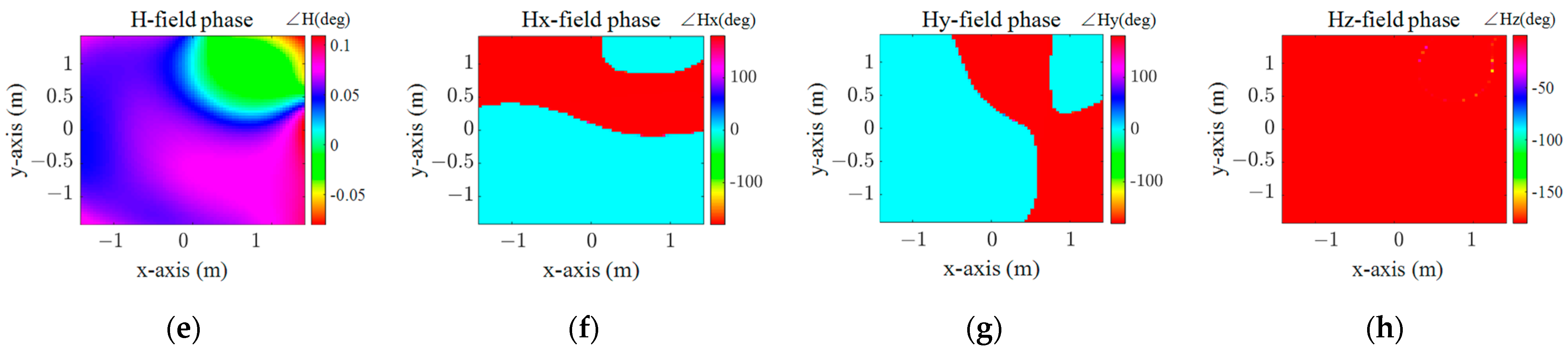
The magnetic field distribution at 120 Hz obtained by simulation: (a) The amplitude distribution of H; (b) The amplitude distribution of Hx; (c) The amplitude distribution of Hy; (d) The amplitude distribution of Hz; (e) The phase distribution of H; (f) The phase distribution of Hx; (g) The phase distribution of Hy; (h) The phase distribution of Hz.
Figure 9.
The magnetic field distribution at 120 Hz obtained by simulation: (a) The amplitude distribution of H; (b) The amplitude distribution of Hx; (c) The amplitude distribution of Hy; (d) The amplitude distribution of Hz; (e) The phase distribution of H; (f) The phase distribution of Hx; (g) The phase distribution of Hy; (h) The phase distribution of Hz.
Figure 10.
The value of the magnetic dipole moment at each frequency: (a) Real(Mx), (b) Real(My), (c) Real(Mz), (d) Imag(Mx), (e) Imag(My), (f) Imag(Mz).
Figure 10.
The value of the magnetic dipole moment at each frequency: (a) Real(Mx), (b) Real(My), (c) Real(Mz), (d) Imag(Mx), (e) Imag(My), (f) Imag(Mz).
Figure 11.
The magnetic field at 120 Hz obtained by the proposed hybrid modeling method is: (a) The amplitude distribution of H; (b) The amplitude distribution of Hx; (c) The amplitude distribution of Hy; (d) The amplitude distribution of Hz; (e) The phase distribution of H; (f) The phase distribution of Hx; (g) The phase distribution of Hy; (h) The phase distribution of Hz.
Figure 12.
Comparison of simulated and computed values on the measurement line: (a) Comparison of the magnetic field intensity at the measured line, (b) Relative error at the measured line.
Figure 12.
Comparison of simulated and computed values on the measurement line: (a) Comparison of the magnetic field intensity at the measured line, (b) Relative error at the measured line.
Table 1.
Advantages and Limitations of Different Equivalent Modeling Methods.
Table 1.
Advantages and Limitations of Different Equivalent Modeling Methods.
Modeling Method
Merits
Limitations
Mode expansion method: The radiation source is equivalent to a superposition of waves of different modes, where the coefficients of each mode can be determined from field data on a known surface.
Good precision.
Ability to analyze different modes of electromagnetic fields.
Difficulty in accurately describing radiation sources with complex structures.
Need for known field data on a closed surface that encloses the radiation source.
Integral equation method: The radiation source is expressed as several integral equations, and then the radiation electromagnetic fields at other locations are derived by solving these equations.
Good precision.
Does not need to consider the boundary conditions.
Long solution time.
Requires knowing field data on a closed surface that encloses the radiation source.
Equivalent electromagnetic current method: By equating the radiation source to the equivalent current or magnetic current source, the electromagnetic field remains consistent with that of the original radiation source.
Accurate characteristics of the magnetic current, continuous current, and distribution on the surface of the radiation source.
Heavy calculation burden.
Cumbersome derivation.
Equivalent dipole method: According to the near-field test data, the electric/magnetic dipole array equivalent model is used to replace the actual radiation source.
Relatively simple method.
Easy to co-simulate with full-wave analysis software.
Accuracy of model related to the number, distribution of dipoles.
Table 2.
Relative error of the magnetic field.
Table 2.
Relative error of the magnetic field.
Magnetic-Field Component
Hx
Hy
Hz
H
Relative error of amplitude
1.6672 dB
1.6370 dB
1.3680 dB
1.3719 dB
Table 3.
Relative error of the amplitude of the magnetic field.
Table 3.
Relative error of the amplitude of the magnetic field.
Frequency
|Hx|
|Hy|
|Hz|
|H|
120 Hz
1.0099 dB
1.0884 dB
0.9743 dB
0.9952 dB
360 Hz
2.0418 dB
1.8593 dB
1.9881 dB
2.0418 dB
Table 4.
Relative Error of a Wideband Equivalent Model.
Table 4.
Relative Error of a Wideband Equivalent Model.
Interpolation Method
Frequency
|Hx|
|Hy|
|Hz|
|H|
Linear interpolation
150 Hz
0.9991 dB
1.0092 dB
0.9307 dB
1.0130 dB
Spline interpolation
150 Hz
0.9400 dB
1.0354 dB
0.9447 dB
0.9237 dB
Piecewise cubic Hermite interpolation polynomial
150 Hz
0.9025 dB
0.9065 dB
0.8444 dB
0.7780 dB
Linear interpolation
200 Hz
1.0546 dB
0.9867 dB
0.9190 dB
1.1037 dB
Spline interpolation
200 Hz
1.0261 dB
0.8523 dB
0.9991 dB
0.8735 dB
Piecewise cubic Hermite interpolation polynomial
200 Hz
1.0122 dB
0.9626 dB
0.8357 dB
1.0091 dB
Table 5.
Relative Error of the Wideband Equivalent Model.
Table 5.
Relative Error of the Wideband Equivalent Model.
Frequency
Error
Hx
Hy
Hz
H
120 Hz
amplitude
0.6805 dB
0.7214 dB
0.6136 dB
0.6556 dB
120 Hz
phase
0.9525 dB
1.0099 dB
0.8665 dB
0.9158 dB
360 Hz
amplitude
1.0331 dB
1.0884 dB
0.9229 dB
0.9119 dB
360 Hz
phase
1.9950 dB
2.0088 dB
1.8537 dB
1.7208 dB
Table 6.
Relative Error of the Magnetic Field at 8 kHz to 2048 kHz with One Point.
Table 6.
Relative Error of the Magnetic Field at 8 kHz to 2048 kHz with One Point.
Frequency
|H|
|Hx|
|Hy|
|Hz|
16 kHz
1.3355 dB
1.3258 dB
2.0095 dB
1.8768 dB
64 kHz
1.7450 dB
3.2345 dB
2.3235 dB
2.2380 dB
256 kHz
1.3793 dB
2.8971 dB
1.6507 dB
1.6715 dB
1024 kHz
1.3941 dB
2.9207 dB
1.7137 dB
1.7015 dB
Table 7.
Relative Error of the Magnetic Field from 8 kHz to 512 kHz with One Point.
Table 7.
Relative Error of the Magnetic Field from 8 kHz to 512 kHz with One Point.
Frequency
|H|
|Hx|
|Hy|
|Hz|
16 kHz
1.4281 dB
2.8045 dB
2.1068 dB
1.9826 dB
64 kHz
1.8474 dB
3.3841 dB
2.4437 dB
2.3593 dB
256 kHz
1.4391 dB
2.9671 dB
1.7194 dB
1.7357 dB
Table 8.
Relative Error of the Magnetic Field from 8 kHz to 2048 kHz with Two Points.
Table 8.
Relative Error of the Magnetic Field from 8 kHz to 2048 kHz with Two Points.
Frequency
|H|
|Hx|
|Hy|
|Hz|
16 kHz
3.7803 dB
5.3006 dB
3.5910 dB
3.9119 dB
32 kHz
3.4351 dB
4.8687 dB
2.9671 dB
3.3191 dB
1024 kHz
1.4897 dB
2.9702 dB
1.8530 dB
1.8922 dB
Disclaimer/Publisher’s Note: The statements, opinions and data contained in all publications are solely those of the individual author(s) and contributor(s) and not of MDPI and/or the editor(s). MDPI and/or the editor(s) disclaim responsibility for any injury to people or property resulting from any ideas, methods, instructions or products referred to in the content.
Huang, X.; Liu, Q.; Pan, X.; Jin, S.; Chen, H.; Wang, X.; Zhao, F.; A, T.; Chen, L.; Zhang, H.
An Equivalent Modeling Method for Wideband Magnetic Radiation Interference of Power-Electronic Equipment. Electronics2024, 13, 2481.
https://doi.org/10.3390/electronics13132481
AMA Style
Huang X, Liu Q, Pan X, Jin S, Chen H, Wang X, Zhao F, A T, Chen L, Zhang H.
An Equivalent Modeling Method for Wideband Magnetic Radiation Interference of Power-Electronic Equipment. Electronics. 2024; 13(13):2481.
https://doi.org/10.3390/electronics13132481
Chicago/Turabian Style
Huang, Xiaoting, Qifeng Liu, Xin Pan, Shuai Jin, Hao Chen, Xin Wang, Fuyu Zhao, Tengge A, Liang Chen, and Huaiqing Zhang.
2024. "An Equivalent Modeling Method for Wideband Magnetic Radiation Interference of Power-Electronic Equipment" Electronics 13, no. 13: 2481.
https://doi.org/10.3390/electronics13132481
APA Style
Huang, X., Liu, Q., Pan, X., Jin, S., Chen, H., Wang, X., Zhao, F., A, T., Chen, L., & Zhang, H.
(2024). An Equivalent Modeling Method for Wideband Magnetic Radiation Interference of Power-Electronic Equipment. Electronics, 13(13), 2481.
https://doi.org/10.3390/electronics13132481
Note that from the first issue of 2016, this journal uses article numbers instead of page numbers. See further details here.
Article Metrics
No
No
Article Access Statistics
For more information on the journal statistics, click here.
Multiple requests from the same IP address are counted as one view.
Huang, X.; Liu, Q.; Pan, X.; Jin, S.; Chen, H.; Wang, X.; Zhao, F.; A, T.; Chen, L.; Zhang, H.
An Equivalent Modeling Method for Wideband Magnetic Radiation Interference of Power-Electronic Equipment. Electronics2024, 13, 2481.
https://doi.org/10.3390/electronics13132481
AMA Style
Huang X, Liu Q, Pan X, Jin S, Chen H, Wang X, Zhao F, A T, Chen L, Zhang H.
An Equivalent Modeling Method for Wideband Magnetic Radiation Interference of Power-Electronic Equipment. Electronics. 2024; 13(13):2481.
https://doi.org/10.3390/electronics13132481
Chicago/Turabian Style
Huang, Xiaoting, Qifeng Liu, Xin Pan, Shuai Jin, Hao Chen, Xin Wang, Fuyu Zhao, Tengge A, Liang Chen, and Huaiqing Zhang.
2024. "An Equivalent Modeling Method for Wideband Magnetic Radiation Interference of Power-Electronic Equipment" Electronics 13, no. 13: 2481.
https://doi.org/10.3390/electronics13132481
APA Style
Huang, X., Liu, Q., Pan, X., Jin, S., Chen, H., Wang, X., Zhao, F., A, T., Chen, L., & Zhang, H.
(2024). An Equivalent Modeling Method for Wideband Magnetic Radiation Interference of Power-Electronic Equipment. Electronics, 13(13), 2481.
https://doi.org/10.3390/electronics13132481
Note that from the first issue of 2016, this journal uses article numbers instead of page numbers. See further details here.


 ,
, 


