SDP-MTF: A Composite Transfer Learning and Feature Fusion for Cross-Project Software Defect Prediction

Abstract

Software defect prediction is critical for improving software quality and reducing maintenance costs. In recent years, Cross-Project software defect prediction has garnered significant attention from researchers. This approach leverages transfer learning to apply the knowledge from existing projects to new ones, thereby enhancing the universality of predictive models. It provides an effective solution for projects with limited historical defect data. Nevertheless, current methodologies face two main challenges: first, the inadequacy of feature information mining, where code statistical information or semantic information is used in isolation, ignoring the benefits of their integration; second, the substantial feature disparity between different projects, which can lead to insufficient effect during transfer learning, necessitating additional efforts to narrow this gap to improve precision. Addressing these challenges, this paper proposes a novel methodology, SDP-MTF (Software Defect Prediction using Multi-stage Transfer learning and Feature fusion), that combines code statistical features, deep semantic features, and multiple feature transfer learning methods to enhance the predictive effect. The SDP-MTF method was empirically tested on single-source cross-project software defect prediction across six projects from the PROMISE dataset, benchmarked against five baseline algorithms that employ distinct features and transfer methodologies. Our findings indicate that SDP-MTF significantly outperforms five classical baseline algorithms, improving the F1-Score by 8% to 15.2%, thereby substantively advancing the precision of cross-project software defect prediction.

1. Introduction

Software defect prediction is a pivotal automated technique aimed at forecasting bugs within software [1]. It aspires to pinpoint potentially flawed modules during the early development phases of a project. By channeling more resources into the scrutiny and testing of these modules, the approach seeks to safeguard software quality and security, fundamentally cutting down the costs associated with manual testing and condensing the development timeline.

In recent years, the domain of cross-project software defect prediction has attracted substantial attention from the research community as a means to bolster software quality assurance. Cross-project defect prediction (CPDP) is principally designed to circumvent the challenges associated with model construction and data paucity in new project defect predictions, as noted by [2]. It endeavors to apply the knowledge encapsulated in the predictive models of established projects (source projects) to predict defects in new ventures (target projects), offering novel solutions for developers to identify and rectify bugs in the nascent stages of the software development life-cycle.

Current cross-project software predictions grapple with two predominant issues. First, is the prevalent focus on single-feature utilization—either code statistics in isolation or semantic information gleaned solely through source code and deep learning techniques but without integrating both feature sets. Since both code statistics and deep semantic features are derived from source code, each provides a unique insight into the source program’s characteristics. They are mutually enriching, not contradictory; their amalgamation could be key to amplifying prediction precision. Second, significant variations in the development processes, programming languages, and personnel coding habits across projects lead to distinct project data features and potentially wide disparities in data distributions. Thus, bridging the gap between varying projects and transferring knowledge from one project domain to another encapsulates the essence of cross-project defect prediction.

In response to these challenges, this paper introduces a novel cross-project software defect prediction approach rooted in compound transfer learning and feature fusion. Initially, a feature constructor is employed to distill code statistical features and deep semantic features from the Abstract Syntax Tree (AST), fusing them into an integrated feature set. Subsequently, a compound methodology that marries Transfer Component Analysis (TCA+) with domain adaption network is deployed on the feature to facilitate transfer learning, diminishing the distributional skew between source and target domains. The transformed features are then channeled into a classifier to conduct the ultimate categorization, culminating in the cross-project software defect prediction task. This methodology was validated on six projects within the PROMISE dataset and benchmarked against five baseline algorithms that employed diverse features and transfer strategies. The empirical findings corroborate that our proposed SDP-MTF method registers a substantial improvement in the F1-Score, ranging from 8% to 15.2% over baseline algorithms, thereby significantly bolstering the precision of cross-project software defect predictions.

The main contributions of this paper are as follows:

• We propose a cross-project software defect prediction method, SDP-MTF, based on compound transfer and feature fusion. Experiments conducted on two datasets demonstrate that our algorithm effectively enhances the effect of cross-project defect prediction methods.
• We utilize both code metric-based statistical features and source code features derived from AST to construct fused features, serving as the foundation for transfer learning and classification, and mining the relationship between projects and defects from multiple feature perspectives.
• We integrate two feature-level transfer learning methods, TCA+ and Deep Adaptation Network (DAN), to narrow the gap between source and target projects, ensuring the effect of cross-project defect prediction.

The subsequent organization of this paper is as follows: Section 2 reviews related work on cross-project software defect prediction; Section 3 primarily introduces our proposed SDP-MTF method, including the motivation and framework behind the method, feature construction, the process of the two transfer learning methods, and feature fusion; Section 4 details our experimental design, including research questions, baseline comparison algorithms, datasets used, and evaluation metrics; Section 5 presents the experimental results; Section 6 analyses and compares the results of the previous experiment and describes the validity threat and Section 7 concludes the paper with a summary and future outlook.

2. Related Work

Cross-Project Defect Prediction (CPDP) primarily addresses challenges in building new project models and data scarcity within project defect prediction [2]. The earliest studies on the feasibility of CPDP can be traced back to the work of [3], who constructed defect prediction models using different projects from the same development team to explore CPDP’s feasibility. Their findings confirmed that the differences between projects in CPDP are non-negligible. Currently, most cross-project software defect prediction research employs transfer learning, applying models and knowledge established in source projects to target projects for new defect prediction tasks. Next, we briefly introduce research and content related to cross-project software defect prediction using code statistical features and deep semantic features.

2.1. Code Statistical Features

Code statistical features are used in the vast majority of research. These features, also known as software metric elements, are intrinsic attributes related to the external manifestations of code defects, typically associated with software testing and quality assurance, and provide valuable insights into the relationship between defects and software programs. Nam [4] leveraging feature mapping, improved the classic feature-based transfer method TCA [5] in transfer learning and proposed a TCA+ method. This approach maps code statistical feature information between projects to a common space for model building and data normalization, automatically selecting optimal data normalization methods. He [6] conducted research from the perspective of feature dimensions, using feature selection methods to choose different feature subsets, identifying the TOP K features, and analyzing their associations to remove redundant features, thereby ensuring the effectiveness of feature subsets. Ni [7] proposed a cross-project defect method based on feature and instance transfer, using feature clustering and the TrAdaBoost [8] method. They compared numerous classic methods and proved the effectiveness of their approach. Hosseini [9] used approximate methods like local sensitive hashing (LSH) to reduce computational costs in instance selection based on nearest neighbor information and proved the effectiveness of these approximate methods through optimizing hyperparameters. Lei [10] reduced the differences between projects from the perspective of feature engineering, introducing transfer learning technology to build cross-project defect prediction models WCM-WTrA and the multi-source model Multi-WCM-WTrA.

2.2. Deep Semantic Features

With the development of deep learning and natural language processing technologies, researchers have begun processing programming languages with NLP techniques, extracting program semantics to generate intermediate representations, and representing program semantics, syntax structures, and contextual relationships. Deep semantic feature-based code classification tasks can be seen as advanced abstraction tasks of NLP in programming languages, including code clone detection, code smell classification, and defect vulnerability detection. Chen [11] proposed a method to address the challenges of extracting and expressing rich semantics and relationships from error reports in code repair. This method combines neural network RNN with dependency parsers to automatically extract error entities and their relationships from error reports. Wang [12] extracted abstract syntax trees from source code and built FA-AST by enriching original ASTs with explicit control and data flow edges. They applied two different types of graph neural networks (GNNs) to assess the similarity of code pairs for clone detection. Li [13] proposed a method combining search-based automatic program repair with neural machine translation approaches, using redundant hypotheses and correct patch sequences for potential repair statements and introduced a new framework called ARJANMT for automatic Java program repair.

In cross-project software defect prediction, such features can also reveal connections between defect patterns and source code. Wang [14] et al., to bridge the gap between program semantics and defect prediction features, proposed leveraging the powerful representational learning algorithm of deep learning to automatically learn semantic representations from source code. Specifically, they used Deep Belief Networks (DBN) to learn semantic features automatically from token vectors extracted from programs’ Abstract Syntax Trees (ASTs). Li [15] proposed the DP-CNN framework for defect prediction, which uses deep learning for effective feature generation and evaluated F1-Score in defect prediction across seven open-source projects, demonstrating superior results compared to DBN. Qiu [16] proposed the Transfer Convolutional Neural Network TCNN, which introduced a distribution matching layer into the process of mining semantic features with convolutional neural networks. By simultaneously minimizing empirical classification loss, cross-project data distribution differences, and manifold regularization, TCNN could extract transferable deep learning-generated features. Gupta [17] extracted seven unique features from programs, evaluated them using Cognitive Complexity Metrics (CCM), and combined the CCM results as node feature values in CFG to create a node vector matrix. This matrix was then fed into a Graph Convolutional Network (GCN) for intermediate representation and defect prediction.

3. Method

3.1. Motivation and Framework

Cross-project software prediction adeptly addresses the issue of missing historical data or the need for early life-cycle software forecasting and has garnered increasing attention from researchers in recent years. Current cross-project software predictions largely employ transfer learning methods, with researchers achieving notable results. However, two main challenges persist in cross-project software defect prediction: incomplete feature construction and significant probability distribution gaps between source and target projects.

In terms of feature construction, existing studies tend to choose either code statistical features or semantic features. Code statistical features are derived from metrics associated with the source code, measuring various indicators of software quality, while semantic features represent the theoretical units that convey the meanings of tokens in the code and their context. Code statistical and semantic features each represent different characteristics of the code from the perspectives of expert knowledge on software quality and the intrinsic structure of the code, respectively. Neglecting either aspect undoubtedly results in the loss of a wealth of rich information, diminishing the precision of predictions.

The gap between source and target projects poses another challenge: cross-project software defect prediction models are built on different projects and cannot directly use data for modeling. Consequently, transfer learning models that migrate knowledge from one domain to another are a common solution. On this premise, deciding what knowledge to transfer and how to further narrow the probability distribution gap between source and target projects to enhance the effect of defect prediction is the core issue in transfer learning-based cross-project software prediction.

Addressing these issues and with the goal of further enhancing the accuracy of cross-project software defect prediction, we propose SDP-MTF, a method that combines transfer learning with feature fusion. Our aim is to improve the final prediction effect from multiple perspectives by utilizing different types of features and suitable transfer learning. Our motivation is to mine as much information as possible from the source and target projects during the feature stage, then apply appropriate transfer learning methods to bridge the gap between the source and target projects, construct suitable transfer features, and ultimately perform defect prediction classification based on this foundation.

The framework of the method we propose is illustrated in Figure 1. The method mainly consists of a feature construction part and a transfer learning part. Firstly, in the feature construction part, we collect code statistical features and semantic features. We use transfer component analysis to transform and map the features of the code statistical features, after which the source code is converted into an intermediate representation of the abstract syntax tree AST, and the semantic features are extracted from the traversal sequences of the AST using Bi-LSTM with a self-attention mechanism. Finally, the two are feature fused to construct a richer and more comprehensive feature representation. This is followed by the transfer learning phase. In this phase, we introduce the domain-adaptive deep adaptive network DAN to train and classify the tasks in the two domains to accomplish the cross-project software defect prediction task. The algorithmic flow of SDP-MTF is shown in Algorithm 1. We will now delineate the details of our method in the subsequent sections.

Algorithm 1 SDP-MTF Methodology
Input:
S: Source project data
T: Target project data
Output:
M: Trained defect prediction model
1.	Parse source code S to obtain code metrics
2.	Apply TCA+ to normalize and transform code metrics
3.	Parse source code S to obtain ASTs
4.	Perform depth-first traversal on ASTs to obtain path sequences
5.	Use Bi-LSTM with self-attention to extract semantic features from path sequences
6.	Concatenate statistical features and semantic features to form a comprehensive feature set
7.	Minimize classifier loss $L_{\mathrm{task}}$: Binary cross-entropy on source domain data
8.	Minimize adaptive loss $L_D$: MK-MMD to reduce distribution differences
9.	Minimize streamform regularization $L_M$: Maintain local similarity structures
10.	Train a classifier on the transformed features
11.	Use the classifier to predict defects in the target project T

3.2. Feature Generation Phase

Next, we describe the details of the method in detail. Figure 2 illustrates the process of the feature construction phase. First, is the feature construction phase, which aims to construct fusion features with richer and more complete information. This phase consists of three steps, namely TCA+-based code statistics feature generation, AST-based semantic feature generation, and feature fusion.

Code statistical features are closely related to the external defects of the code and are another name for software metrics. Typically, each metric is related to certain functional features of a software project, such as coupling, cohesion, inheritance, and code modification [18], which characterize a software product macroscopically. They provide a basis for improving software quality and efficiency through data analysis. Metrics are crucial for cross-project software defect prediction, offering key data to identify patterns, predict high-risk areas, and help teams detect issues early, optimize testing, and enhance software quality.

Code statistical features are selected and extracted by humans, and their quality is directly related to a priori expert knowledge. We used some of the code statistics created by Jureczko et al. [19] and shared in PROMISE. Specific descriptions of the code statistics used by SDP-MTF are shown in

Table 1. The description of the code statistics used by the SDP-MTF.

Feature Name	Feature Description
amc	The average complexity of methods.
avg_cc	The average McCabe Cyclomatic Complexity in a file.
cam	The sum of the number of parameters of different types of methods.
cbm	The number of inter-method couplings.
cbo	The number of inter-object couplings.
ce	The number of outward coupling.
dam	The ratio of the number of private attributes to the total number of attributes.
dit	The depth of the inheritance tree.
ic	The number of inheritance couplings.
lcom	The number of lack of cohesion between methods.
lcom3	The another measure of the lack of method cohesion.
loc	The number of lines of code.
max_cc	The McCabe maximum cyclomatic complexity.
mfa	The number of function abstractions.
moa	The number of data declarations counted.
noc	The number of subclasses of a class.
npm	The number of public methods.
rfc	The number of methods called in response to a message.
wmc	The number of methods in a class (assuming all methods have a weight of 1).

.

After that, for the differences in code statistics between different projects, we use the classical transfer component analysis method, TCA+ [5], to find the migratable components between different projects, and reduce the differences between different projects while preserving the structural characteristics of the data. The core idea of TCA+ is to learn the transformation of mapping the data of the source and target projects into the Reproducing Kernel Hilbert Space (RKHS), which is the most efficient method to analyze the data of source and target projects. into the Reproducing Kernel Hilbert Space (RKHS) transformations. In this space, the maximum mean difference $Dist(\phi \left(X_s\right),\phi \left(X_T\right))$ between the source project’s feature $X_s$ and the target project’s feature $X_T$ is very small and the variance of the transformed data $Var\left(\phi \left(X_s\right),\phi \left(X_T\right)\right)$ is very large, and the formula for the optimization objective can be abstracted as:

$$\begin{array}{c}\hfill argmi{n}_{\phi }Dist(\phi \left(X_S\right),\phi \left(X_T\right))+\lambda R\left(\phi \right)\end{array}$$

where $R\left(\phi \right)$ is the regularization term to avoid overfitting, and $\lambda \ge 0$ is the tradeoff parameter that controls the effect of the regularization term in the target. We refer to the retained source and target project features after the TCA+ transformation as source project statistical features and target project code statistical features for subsequent feature fusion.

In order to compensate for the problems of insufficient feature information mining and single feature type, we introduce semantic features of source code to supplement. Semantic features of source code refer to the meaningful aspects of code that convey its functionality and behavior. These include the types of nodes (such as variable declarations, function calls, and control structures), identifiers (names of variables, functions, and classes), operators (arithmetic, logical, and assignment operators), and constants (numerical values, strings, etc.). These features help in understanding the logic and intent of the code, making them crucial for tasks such as defect detection, code analysis, and optimization. By extracting these semantic features, we can enhance the comprehensiveness and accuracy of our analysis.

We extract semantic information of source and target projects based on the Abstract Syntax Tree (AST) sequence. First, we parse the source codes of different projects using JavaLang, obtain their ASTs and perform depth-first traversal to obtain the path sequences. The path sequence contains the global information of the source code with the syntactic structure features of the source code.

We use Bi-LSTM to learn the contextual features of the AST sequences. Bi-LSTM is a commonly used deep semantic model for contextual semantic capture and belongs to the RNN network. Compared with unidirectional LSTM, Bi-LSTM not only inherits the function of LSTM in capturing the semantics of long sequences, but also solves the limitation of LSTM in the coding from the back-to-front direction, and is able to capture the semantics between statements more effectively from the back-to-front direction to capture the semantic dependencies between utterances. Bi-LSTM at each position t can be described and computed by the following equation.

$$\begin{array}{cc}\hfill i_t& =\sigma (W_i·[h(t-1),x_t]+b_i)\hfill \end{array}$$

(1)

$$\begin{array}{cc}\hfill f_t& =\sigma (W_f·[h(t-1),x_t]+b_f)\hfill \end{array}$$

(2)

$$\begin{array}{cc}\hfill o_t& =\sigma (W_o·[h(t-1),x_t]+b_o)\hfill \end{array}$$

(3)

where $\sigma (·)$ represents the sigmoid function, $x_t$ denotes the sequence of statements at position t and $h_t$ represents the learning assumption of the hidden layer. The $c_t$ represents the unit of the hidden layer with the learning assumption of the hidden layer $h_t$ can be calculated by the following equation:

$$\begin{array}{cc}\hfill \widetilde{c_t}& =tanh(W_c·[h(t-1),x_t]+b_c)\hfill \end{array}$$

(4)

$$\begin{array}{cc}\hfill c_t& =f_t\odot c(t-1)+i_t\odot \left(c_t\right)\hfill \end{array}$$

(5)

$$\begin{array}{cc}\hfill h_t& =o_t\odot tanh\left(c_t\right)\hfill \end{array}$$

(6)

Finally, Bi-LSTM performs forward and backward traversal of the inputs and sums the results, and the final result can be expressed by the following equation:

$$\begin{array}{c}\hfill h_i=[\overrightarrow{h_i}\oplus \overleftarrow{h_i}]\end{array}$$

(7)

After extracting the context information, we introduce the self-attention mechanism [20] to solve the dependency problem caused by the long distance of the context vocabulary and can effectively extract the internal connection between statements. The self-attention mechanism can be expressed by the following formula:

$$\begin{array}{c}\hfill Attention(Q,K,V)=Softmax\left(\frac{Q{K}^T}{\sqrt{d_k}}\right)V\end{array}$$

(8)

where $d_k$ represents the dimension of the hidden representation and Q, K, V are linear functions of the previously hidden representation, generated from the embedding paths, that is, the

$$\begin{array}{cc}\hfill Q& =H^{l-1}{W}_Q^l,Q\in R^{l\times d}\hfill \end{array}$$

(9)

$$\begin{array}{cc}\hfill K& =H^{l-1}{W}_K^l,K\in R^{l\times d}\hfill \end{array}$$

(10)

$$\begin{array}{cc}\hfill V& =H^{l-1}{W}_V^l,V\in R^{l\times d}\hfill \end{array}$$

(11)

After obtaining the code statistical features and semantic features of the source and target projects through the above steps, the final fusion features are obtained by using the means of splicing, and the fusion features can be described as:

$$\begin{array}{c}\hfill featur{e}_{all}=concat(featur{e}_s,featur{e}_c)\end{array}$$

(12)

where ${feature}_s$, ${feature}_c$ represent the statistical features of the migrated code and the semantic features generated in depth based on the abstract syntax tree, respectively, and $contact$ is the splicing operation.

3.3. Transfer Learning Phase

After obtaining the fusion features, we enter the transfer learning stage. In this stage, we use the idea of Deep Adaptation Neural Network (DAN) [21] in deep transfer learning, and introduce the training model based on domain adaptation [22] for the construction of a cross-project defect prediction model. The schematic of the deep adaptive neural network we used can be shown in Figure 3.

The optimization objective of the DAN model is three complementary objective functions as follows:

(1)

Minimize the classifier loss $L_{task}$ for source domain data;

(2)

Minimize the adaptive loss $L_D$ between the source and target domains;

(3)

Minimize the flow regularization term $L_M$ between the source and target domains;

Therefore, the optimization objective of the deep adaptive neural network DAN can be expressed as:

$$\begin{array}{c}\hfill L_{total}=min(L_{task}+\lambda L_D+\beta L_M)\end{array}$$

(13)

where $\lambda >0$ and $\beta >0$ are two balancing parameters used to balance the effects of classifier loss and adaptive loss, respectively.

The specific formulas for each of the three losses are given next. The first is the classifier loss $L_{task}$ for the source domain data, which uses the binary cross entropy as the loss function for binary categorization, specifically:

$$\begin{array}{c}\hfill L_{task}=-\frac{1}{N_s}\sum _{i=1}^N[y_{i}log\left(\widehat{y_i}\right)+(1-y_i)log(1-\widehat{y_i})]\end{array}$$

(14)

where $N_s$ is the number of source domain samples, $y_i$ is the true label of the ith sample, and $\widehat{y_i}$ is the result of the ith sample predicted by the model.

Next, is the adaptive loss $L_D$ between the source and target domains, which is performed in the last three layers using the multi-kernel maximum mean difference MK-MMD [23] for the difference in distribution between the source and target projects, and the resulting adaptive loss. The adaptive loss for each adaptive layer is as follows:

$$\begin{array}{c}\hfill L_{MMD}={∥\frac{1}{N_s}\sum _{i=1}^{N_s}\varphi \left(x_i^s\right)-\frac{1}{N_t}\sum _{j=1}^{N_t}\varphi \left(x_j^t\right)∥}_{{\mathcal{H}}_{\mathcal{k}}}^2\end{array}$$

(15)

where $N_s$ and $N_t$ represent the number of samples in the source and target domains, respectively, and $\varphi (·)$ is the mapping function that maps the input data into the Hilbert space; $x_i^s$ and $x_j^t$ are the samples in the source and target domains, respectively, and $\mathcal{H}$ denotes the regenerated kernel Hilbert space RKHS, MK- MMD losses are computed in this space. The k represents a linear combination of multiple kernel functions, as follows:

$$\begin{array}{c}\hfill k(x,x^{\prime })=\sum _{q=1}^Q{d}_q{k}_q(x,x^{\prime })\end{array}$$

(16)

where $d_q$ is the weight of the kernel $k_q$, which is used to optimize the distance measure between the two distributions during learning.

In addition, since three adaptive layers are used, the total adaptive loss is as follows:

$$\begin{array}{c}\hfill L_D=\sum _{i=1}^3{L}_{MMD}\end{array}$$

(17)

Finally, there is the stream-form regularization term. The basic assumption of stream-form regularization is that local similarities between data points may not be apparent in a high-dimensional space, but are significant on some low-dimensional stream-form. Based on this premise, stream-form regularization attempts to maintain the local neighborhood structure between data points during the learning process, even when dealing with high-dimensional data [24]. Thus, the stream shape regularization term can be expressed as follows:

$$\begin{array}{cc}\hfill L_M& =\frac{1}{2}\sum _{q=1}^Q{d}_q\left(\sum _{i,j}{W}_{ij}{\parallel {\Phi }_q\left(x_i\right)-{\Phi }_q\left(x_j\right)\parallel }^2\right)\hfill \\ \hfill & =\frac{1}{2}\sum _{q=1}^Q{d}_q\left(Tr\left({\Phi }_q^{T}L{\Phi }_q\right)\right)\hfill \end{array}$$

(18)

where $\varphi \left(x_i\right)$ and $\varphi \left(x_j\right)$ denote the points $x_i$ and $x_j$ mapped to the low-dimensional manifolds, respectively, while $W_{ij}$ is the similarity matrix representing the similarity between the points $x_i$ and $x_j$, and L is the normalized Laplace matrix. $d_q$ is the kernel weight used to weigh the contribution of different kernel functions in MK-MMD and Q is the number of different kernel functions used. The $k_q$ represents the kernel functions, each of which provides a view from a different feature space and is used to learn and compare the difference in distribution between the source and target domains.

Finally, the similarity matrix $W_{ij}$ is computed as follows:

$$\begin{array}{c}\hfill W_{ij}=\left\{\begin{array}{cc}cos(x_i,x_j)\hfill & \mathrm{if}{x}_i\in N_k\left(x_j\right)\vee x_j\in N_k\left(x_i\right)\hfill \\ \\ 0\hfill & \mathrm{otherwise}\hfill \end{array}\right.\end{array}$$

(19)

where $cos(x_i,x_j)$ denotes the cosine similarity between the vector $x_i$ and the vector $x_j$. $(N_k\left(x_j\right)$ denotes the set of k vectors that are most similar to vector $x_j$, i.e., the k nearest neighbors of $x_j$. The weight $W_{ij}$ is set to the cosine similarity between $x_i$ and $x_j$ when $x_i$ and $x_j$ are k-nearest neighbors, otherwise, it is set to 0. This approach, which considers only the similarity between each point and its k-nearest neighbors, helps to focus on the local structure of each data point when constructing the network and ignores the relatively distant and less relevant points.

Therefore, the total loss function optimization of the prediction model can be expressed as:

$$\begin{array}{cc}\hfill \Theta =& \underset{\Theta }{argmin}{L}_{\mathrm{task}}+\lambda L_D+\beta L_M\hfill \\ \hfill =& -\frac{1}{N_s}\sum _{i=1}^{N_s}\left[y_{i}log\left(\widehat{y_i}\right)+(1-y_i)log(1-\widehat{y_i})\right]\hfill \\ \hfill & +\lambda \sum _{i=1}^3{∥\frac{1}{N_s}\sum _{i=1}^{N_s}\varphi \left(x_i^s\right)-\frac{1}{N_t}\sum _{j=1}^{N_t}\varphi \left(x_j^t\right)∥}_{mathcalH}^2\hfill \\ \hfill & +\frac{\beta }{2}\sum _{i,j}{W}_{ij}{\parallel \varphi \left(x_i\right)-\varphi \left(x_j\right)\parallel }^2\hfill \end{array}$$

(20)

We input the output of the DAN to a fully connected layer that, along with the project label columns, serves as the input to the classifier to accomplish the final prediction of cross-project defects. We chose SVM as the classifier, which has some advantages in handling high-dimensional data.

4. Experiments Design

In this section, we will introduce the research questions, dataset, experimental baselines, and evaluation metrics that our experiments will explore.

4.1. Research Questions

Our experimental motivation is to investigate the effectiveness of our method in various aspects. Therefore, we propose the following questions and conduct experiments around them.

RQ1: How does our proposed method compare to the baseline algorithms in cross-project software defect prediction? RQ1 is our most critical research question, aimed at exploring the comparison between our method and the baseline approach. For baseline algorithms, we examined classical methods in cross-project software defect prediction, with their names and descriptions provided in Section 4.3. In Section 5.1, we will compare the performance of our proposed SPD-MTF method with the baseline algorithms based on evaluation metrics.

RQ2: Does our method of using fused features effectively enhance the predicted effect of cross-project software defect prediction? RQ2 aims to explore whether our proposed method of feature fusion truly improves the effect of cross-project software defect prediction. Our approach suggests using both code statistical features and deep semantic features simultaneously, merging them into a new feature set to mine more information within projects to enhance the final prediction effect. We will conduct experiments around RQ2 to compare the impact of using code statistical features alone, semantic features alone, and our method on defect prediction effect. Section 5.2 presents specific data and conclusions of these experiments.

RQ3: How does the dimensionality of the fused features of SDP-MTF affect cross-project software defect prediction effect? RQ3 aims to explore the impact of the dimensionality of the fused features of SDP-MTF on the model effect. The fused features used in SDP-MTF consist of two parts, namely, the coded statistical features with feature transfer and the AST-based semantic features, and the two features are connected to form the final fused features using the $contact$ operation, and we will explore the impact of the dimensionality of the two feature vectors on the final effect, respectively. The results and analysis of this RQ are shown in Section 5.3.

RQ4: Does our proposed compound method based on domain multiple transfer learning effectively improve the effect of cross-project software defect prediction? In RQ4, we investigate the impact of our proposed method combining domain adaptation transfer learning and feature transfer on the final defect prediction effect. In this research question, we will compare methods that do not use a discriminator and directly use fused features for defect prediction, with methods that use a discriminator but do not perform feature transfer on code statistical features, and the performance of SDP-MTF. Section 5.4 elucidates the specific performance of these experiments.

4.2. Dataset and Evaluation Metrics

We use the commonly used PROMISE dataset in software defect prediction as our dataset [19]. The PROMISE dataset contains open-source project codes, collected by Jureczko and Madeyski and available from the PROMISE data repository. We selected six projects, all written in JAVA, and obtained the source code and code statistical features from the dataset.

Table 2. The Dataset.

Project	Version	Amount	Defect Percentage
Camel	1.6	935	20.10%
Poi	3.0	438	64.10%
Xerces	1.4.4	508	76.80%
Lucene	2.4	330	61.50%
Xalan	2.6	875	53.10%
Log4j	1.2	194	95.90%

shows the names, versions, sizes, and defect rates of the projects used.

On the evaluation indicators of the supervised classification model, we used the F1-Score. Its formula is as follows:

$$\begin{array}{c}\hfill F1\text{-}Score=\frac{2\times Precision\times Recall}{Precision+Recall}\end{array}$$

(21)

Among them, Precision represents the accuracy of the positive predictions made by the model, while Recall refers to the proportion of actual positive cases that were correctly identified by the model. The formulas for these metrics are as follows:

$$\begin{array}{cc}\hfill Precision=& \frac{TP}{TP+FP}\hfill \end{array}$$

(22)

$$\begin{array}{cc}\hfill Recall=& \frac{TP}{TP+FN}\hfill \end{array}$$

(23)

Finally, in order to assess the generalization ability and stability of the algorithm over different cross-project pairs, this paper also uses the IQR Range (IQR) in statistical learning to qualitatively assess the algorithmic metrics in terms of dispersion, outliers, and consistency. The IQR is the difference between the third quartile (Q3) and the first quartile (Q1) and is given by the equation:

$$IQR=Q3-Q1$$

(24)

Regarding the composition of cross-project software defect prediction tasks, we first select one project from the dataset as the target project and then use the remaining five projects as source projects, forming 30 pairs of cross-project software defect prediction tasks with six open-source projects.

4.3. Baseline

In selecting baseline methods, we chose to compare various representative cross-project software prediction methods, including algorithms that solely use code statistical features like TCA [4] and NNFilter [25], algorithms that exclusively use deep semantic features like DBN [26] and AC-GAN [27], and an algorithm that combines both types of features, CNN-THFL [16] and BATM [28].

Table 3. The information of baseline algorithm.

Algorithm	Author	Year	Features	Training Model
NNFilter	[25]	2009	Statistic feature	Naive Bayes
TCA	[5]	2013	Statistic feature	Transfer Component Analysis (TCA)
DBN	[26]	2018	Deep sematic feature	Deep Belief Network (DBN)
AC-GAN	[27]	2022	Deep sematic feature	Generative Adversarial Network (GAN)
CNN-THFL	[16]	2019	Statistic feature and deep semantic feature	TCA + CNN
BATM	[28]	2024	Statistic feature and deep semantic feature	Adversarial Learning

lists the selected baseline algorithms and their brief information.

TCA and NNFilter are classic methods for cross-project software defect prediction using only code statistical features, laying a solid foundation for this prediction approach. TCA+ is a variant of the classic feature transfer algorithm TCA, adapted for prediction tasks, aiming to extend the application of the TCA algorithm using custom data preprocessing rules and regularization terms. NNFilter applies instance transfer in software defect prediction, filtering out source project data unrelated to the target project to make the data distribution between projects more similar.

For algorithms using only deep semantic features, we selected DBN and AC-GAN. DBN utilizes Deep Belief Networks (DBN) to automatically learn semantic features from token vectors extracted from program abstract syntax trees and source code changes. AC-GAN, after extracting semantic word vectors from the abstract syntax tree of the source code, employs adversarial learning for feature extraction and data transfer to complete defect prediction tasks.

Finally, as mentioned earlier, there are a few methods that fuse code statistical and deep features. We selected two algorithms for comparison. CNN-THFL mines deep learning-generated features from token vectors extracted from program abstract syntax trees through convolutional neural networks, then adds code statistical features for feature fusion and utilizes TCA for transferable joint features. BATM also employs a method that uses both types of features simultaneously. They introduce pseudo-labels and an auxiliary classifier, ensuring the model’s predictive performance across different projects through adversarial training.

To ensure the validity of our experiments, we ran the above methods under the same experimental conditions as our proposed SDP-MTF, adjusting according to the parameters described in the papers to ensure that the experimental data are recorded when each model is in its optimal state.

5. Experimental Results

In this chapter, we will explore the four research questions (RQs) proposed in Section 4.1, demonstrating the effectiveness of our model from various perspectives.

5.1. Model Prediction Result

In response to the question raised in RQ1, we compare our method with the baseline algorithms mentioned in Section 4.3, using the F1-Score as the evaluation metric, as specified in Section 4.2. For each experiment, we use one project as the target project and each of the other five projects as the source project, conducting single-source cross-project defect prediction experiments. The results of all single-source cross-project software defect predictions are presented in

Table 4. The F1-Score of SDP-MTF with baseline algorithm.

Source Project	Target Project	SDP-MTF	NNFilter	TCA+	DBN	AC-GAN	CNN-THFL	BATM
Log4j	Camel	0.3988	0.2044	0.2208	0.2477	0.3100	0.2690	0.3045
Lucene		0.3969	0.3204	0.3040	0.2765	0.4256	0.3565	0.4453
Poi		0.3459	0.2871	0.3160	0.3272	0.3384	0.2782	0.3339
Xalan		0.3497	0.3033	0.3057	0.2746	0.3180	0.3302	0.3502
Xerces		0.4296	0.3146	0.2882	0.2917	0.3546	0.3142	0.4245
Camel	Log4j	0.7660	0.6065	0.5758	0.6034	0.7699	0.6679	0.7286
Lucene		0.7851	0.5925	0.5833	0.6100	0.7603	0.6323	0.7961
Poi		0.8016	0.5771	0.6422	0.6308	0.7592	0.6208	0.6586
Xalan		0.7593	0.8303	0.8040	0.8018	0.8125	0.7835	0.7229
Xerces		0.7852	0.5923	0.6895	0.6295	0.7045	0.7069	0.7187
Camel	Lucene	0.7466	0.5142	0.6024	0.5691	0.7434	0.6100	0.7259
Log4j		0.7424	0.5914	0.5379	0.5408	0.6532	0.5605	0.6606
Poi		0.7268	0.5620	0.6404	0.5617	0.7011	0.6829	0.6037
Xalan		0.7935	0.7063	0.7158	0.6543	0.4886	0.6903	0.6065
Xerces		0.7783	0.6141	0.5962	0.5401	0.6260	0.6756	0.7193
Camel	Poi	0.7396	0.4576	0.5752	0.5735	0.7058	0.6590	0.5847
Log4j		0.7561	0.6570	0.3981	0.5670	0.6907	0.5205	0.6950
Lucene		0.7796	0.6195	0.7343	0.5516	0.6575	0.6324	0.6151
Xalan		0.7966	0.7704	0.5981	0.6858	0.7243	0.7455	0.7764
Xerces		0.7555	0.7254	0.5081	0.5811	0.7195	0.5864	0.6688
Camel	Xalan	0.7592	0.5686	0.5454	0.6182	0.4930	0.6858	0.6771
Log4j		0.7822	0.7089	0.6278	0.7447	0.7542	0.7424	0.6503
Lucene		0.7984	0.6100	0.6024	0.6142	0.5576	0.6495	0.6708
Poi		0.7816	0.5004	0.6026	0.6266	0.7312	0.6364	0.7066
Xerces		0.7325	0.5844	0.7068	0.6268	0.5815	0.6823	0.6747
Camel	Xerces	0.7663	0.5039	0.5595	0.5609	0.6168	0.6521	0.7139
Log4j		0.7825	0.7128	0.7107	0.5470	0.6864	0.6535	0.7081
Lucene		0.7701	0.6886	0.6563	0.5113	0.7029	0.6904	0.6544
Poi		0.7908	0.5858	0.6389	0.5551	0.7655	0.7158	0.6716
Xalan		0.7864	0.7310	0.7849	0.7023	0.6295	0.6517	0.6720
Avg		0.7061	0.5680	0.5690	0.5542	0.6261	0.6028	0.6290

. We used a bold font to indicate the best-case scenario for this cross-project prediction.

In all the comparison experiments, our proposed SDP-MTF method achieves the highest average F1-Score of 0.7061, which is on average 8% to 15.2% better than other algorithms. Meanwhile, in all but three cross-project pair experiments, “Lucene → Camel”, “Camel → Log4j” and “Xalan → Log4j”, SDP-MTF achieves the highest average F1-Score of 0.7061, which is 8% to 15.2% higher than other algorithms. SDP-MTF achieves the highest precision and F1-Score. Specifically, SDP-MTF improves F1-Score by up to 28.2% and 13.8% on average compared to the NNFilter algorithm; it improves F1-Score by up to 35.8% and 13.7% on average compared to the TCA+ algorithm; compared to the DBN algorithm, SDP-MTF improves F1-Score by up to 25.6% of F1-Score, with an average improvement of 15.2% of F1-Score; for AC-GAN, SDP-MTF improves up to 30.5% of F1-Score, with an average improvement of 8% of F1-Score, and the algorithm outperforms SDP-MTF on three project pairs, making it the best performing algorithm among the compared algorithms. Finally, CNN-THFL and BATM, similar to SDP-MTF, use the idea of combining statistical features with semantic features, and in terms of F1-Score, SDP-MTF improves 23.6% to CNN-THFL, with an average of 10.3%, and vs. BATM, SDP-MTF improves up to 30%, with an average of 5.6% on average.

Figure 4 shows the stability of each algorithm’s F1-Score on different target projects. We show the maximum, minimum, and median values of each algorithm’s F1-Score under different source projects when each project is the target project, as well as the stability of different algorithms in terms of IQR. The boxplots with different projects as target projects are separated by dashed lines, where the six different algorithms are distinguished by different colors. In this case, Figure 4a shows the performance of the algorithms when the target project is Camel, Log4j and Lucene, while Figure 4b demonstrates the case of the algorithms when the target project is Poi, Xalan and Xerces.

Combining the information from the above pictures, Camel has a large difference in F1-Score from the other projects, so in the subsequent discussion, we will focus on the cross-project pairs with the other projects as the target projects, and the reasons for the poor performance of Camel’s project will be discussed in the final analysis section. In the cross-project prediction except Camel, the SDP-MTF algorithm shows the best results with the smallest IQR, i.e., the best stability, and has the highest rankings on the majority of the project pairs, and the IQR is small on each target project, and the IQR for the F1-Score is 0.02, which is ranked the second best among all algorithms, and has a good stability and generalization ability.

For the other six comparative baseline algorithms. BATM, which uses two features with adversarial learning, was ranked second with an F1-Score of 0.6290. It is ranked fourth for stability with an IQR of 0.1082. And then is followed by AC-GAN, which employs the idea of adversarial learning, and is ranked third in terms of average F1-Score performance, while the algorithm is generally stable, with an IQR of 0.15 for the F1-Score, and is ranked fifth overall. The algorithm that ranked fourth in prediction effectiveness is CNN-THFL, an algorithm that also uses statistical features and semantic features of the code, and the algorithm has an IQR of 0.06, for the F1-Score, and ranks third in stability. The fifth and sixth-ranked algorithms are TCA+ and NNfilter which use coded statistical features and transfer learning of statistical features from the perspective of features and instances, respectively, and both perform poorly in terms of stability performance, with an IQR of 0.24 for the F1-Score of NNFliter, and 0.23 for the TCA+ algorithm, respectively. The final algorithm that performs poorly in our experiments is DBN which uses semantic features alone, with an IQR of 0.06, and ranked third in terms of stability. The algorithm that performed less well in our experiments was DBN with semantic features alone, with an average F1 value of 0.594, but this algorithm was the most stable with an IQR of 0.01 for the F1-Score.

The performance of the baseline algorithms also gives some useful information: first, the first and second-ranked algorithms are SDP-MTF and AC-GAN, while the DBN method using semantic features alone is slightly insufficient in terms of F1-Score, which side by side indicates that the semantic features need to be learned and processed further during the transfer process, and also need to be supplemented with deep transfer learning for cross-project coordination; second, the same as SDP- MTF also using the method BATM CNN-THFL that combines code statistical features and semantic features performs better than NNfilter, TCA+ algorithm that uses code statistical features alone and DBN algorithm that uses semantic features alone, which proves that the use of the combination of code statistical features and semantic features can improve the F1-Score and validates the motivation of our proposed method. We will discuss the project and algorithm effects in more depth in the subsequent analysis.

RQ1 Results: Our proposed SDP-MTF method outperformed the baseline algorithms in terms of F1-Score, ranking second in stability among all algorithms.

5.2. Impact of Fusion Features on the Experimental Model

This subsection develops ablation experiments for RQ2, aiming to explore whether our proposed feature fusion approach improves the effect of cross-project software defect prediction.

Table 5. The F1-Score for SDP-MTF and algorithms using features alone.

Source Project	Target Project	SDP-MTF	SDP-DS	SDP-CS
Log4j	Camel	0.3988	0.3805	0.3668
Lucene		0.3969	0.3648	0.3668
Poi		0.3459	0.3319	0.3213
Xalan		0.3497	0.3249	0.4063
Xerces		0.4296	0.3842	0.3901
Camel	Log4j	0.7660	0.7063	0.7335
Lucene		0.7851	0.7057	0.6918
Poi		0.8016	0.6554	0.7208
Xalan		0.7593	0.6780	0.6169
Xerces		0.7852	0.6685	0.6531
Camel	Lucene	0.7466	0.7287	0.6735
Log4j		0.7424	0.6628	0.6031
Poi		0.7268	0.6609	0.6115
Xalan		0.7935	0.7190	0.6630
Xerces		0.7783	0.7013	0.6555
Camel	Poi	0.7396	0.6552	0.5919
Log4j		0.7561	0.7394	0.6268
Lucene		0.7796	0.7016	0.6432
Xalan		0.7966	0.7302	0.6804
Xerces		0.7555	0.6989	0.6564
Camel	Xalan	0.7592	0.6564	0.5793
Log4j		0.7822	0.6940	0.6278
Lucene		0.7984	0.6883	0.6058
Poi		0.7816	0.6376	0.5037
Xerces		0.7325	0.6535	0.5943
Camel	Xerces	0.7663	0.6605	0.7212
Log4j		0.7825	0.6622	0.6402
Lucene		0.7701	0.7036	0.6537
Poi		0.7908	0.7253	0.6762
Xalan		0.7864	0.6546	0.6941
Avg		0.7061	0.6311	0.5990

shows the F1-Score of the algorithm for SDP-MTF versus the algorithm using a feature alone. SDP-MTF uses a combination of code statistical features and semantic features to fuse them into new features that mine more information within the project to improve the final prediction effect. We compare the performance of the algorithms SDP-DS (Deep-learning based Semantic Feature) using semantic features alone, SDP-CS (Code Statistic Feature) using code statistical features alone, and SDP-MTF with fused features through ablation experiments. The first two columns of the table represent the source and target projects, the third to last column is the F1-Score, and the last row represents the average performance of each algorithm.

It is easy to see that SDP-MTF using fused features outperforms SDP-DS using semantic features alone and SDP-CS using code statistical features alone, while comparing SDP-DS and SDP-CS, they perform similarly, with SDP-DS using only semantic features slightly outperforming SDP-CS using code statistical features alone. The average SDP-DS F1-Score using only semantic features is 0.6311, which is 7.4 percentage points lower than the SDP-MTF algorithm. The average F1-Score of the SDP-CS algorithm using code statistical features alone is 0.5990, which is 10.7 percentage points lower than the SDP-MTF algorithm using fused features. On the algorithm using code semantic and statistical features alone, the semantic features are slightly better but still have a large gap with the fusion features, which proves the effectiveness of the fusion features, and verifies that a single type of feature will lead to a lower effect, and also verifies our view that there is a need for complementary information between the two features.

The bars in Figure 5 represent, from left to right, the fusion feature algorithm SDP-MTF, the semantic feature alone SDP-DS, and the code statistical feature alone SDP-CS. From the figure, we can see that the stability of SDP-MTF is better than that of SDP-DS with the semantic feature alone and SDP-CS with the code statistical feature alone. CS, with the smallest IQR, which we believe is related to the introduction of multiple types of features, compensates for the feature information while improving the generalization ability of the model. The four-digit scores of SDP-DS and SDP-CS are similarly spaced, specifically, the IQR of the SDP-DS F1-Score with semantic features only is 0.07, while the IQR of the SDP-CS with code statistical features only is 0.08.

From the comparison in RQ2, we can draw the following informative conclusion: the prediction effect using fused features is higher than the result of using a feature alone while keeping other experimental conditions constant. Meanwhile, our experiments also answer RQ2 that the use of fusion features can effectively improve the prediction effect of the model, and under the same experimental conditions, the prediction effect is better than the effect of the model that uses semantic features and code statistics features alone. Fusion features can be more effective in solving the problem of a single type of feature, and at the same time, the introduction of fusion features can make the feature information more comprehensive, effectively making up for the problem of insufficient feature information mining.

RQ2 Result: Our proposed method of using fusion features is effective and can significantly improve the prediction effect of cross-project defects when comparing the models using code statistical features alone and semantic features alone.

5.3. Impact of Feature Dimensions on Model Result

This subsection conducts experiments for RQ3 with the aim of exploring the impact of the dimension of the fusion features of SDP-MTF on the effect of the model. The fusion features we use consist of two parts, the coded statistical features with feature transfer and the AST-based semantic features, in this subsection, the generated dimensions of the semantic features are directly generated using Bi-LSTM control, whereas the dimensions of the statistical features are usually reduced or unchanged after feature transfer, and we will use a fully connected layer to control the length of the statistical features. We use Statistic to represent the code statistical features for the upper part of the fusion features, and Deep Semantic to represent the semantic features for the lower part of the fusion features and use the F1-Score as the judging metrics for this experiment.

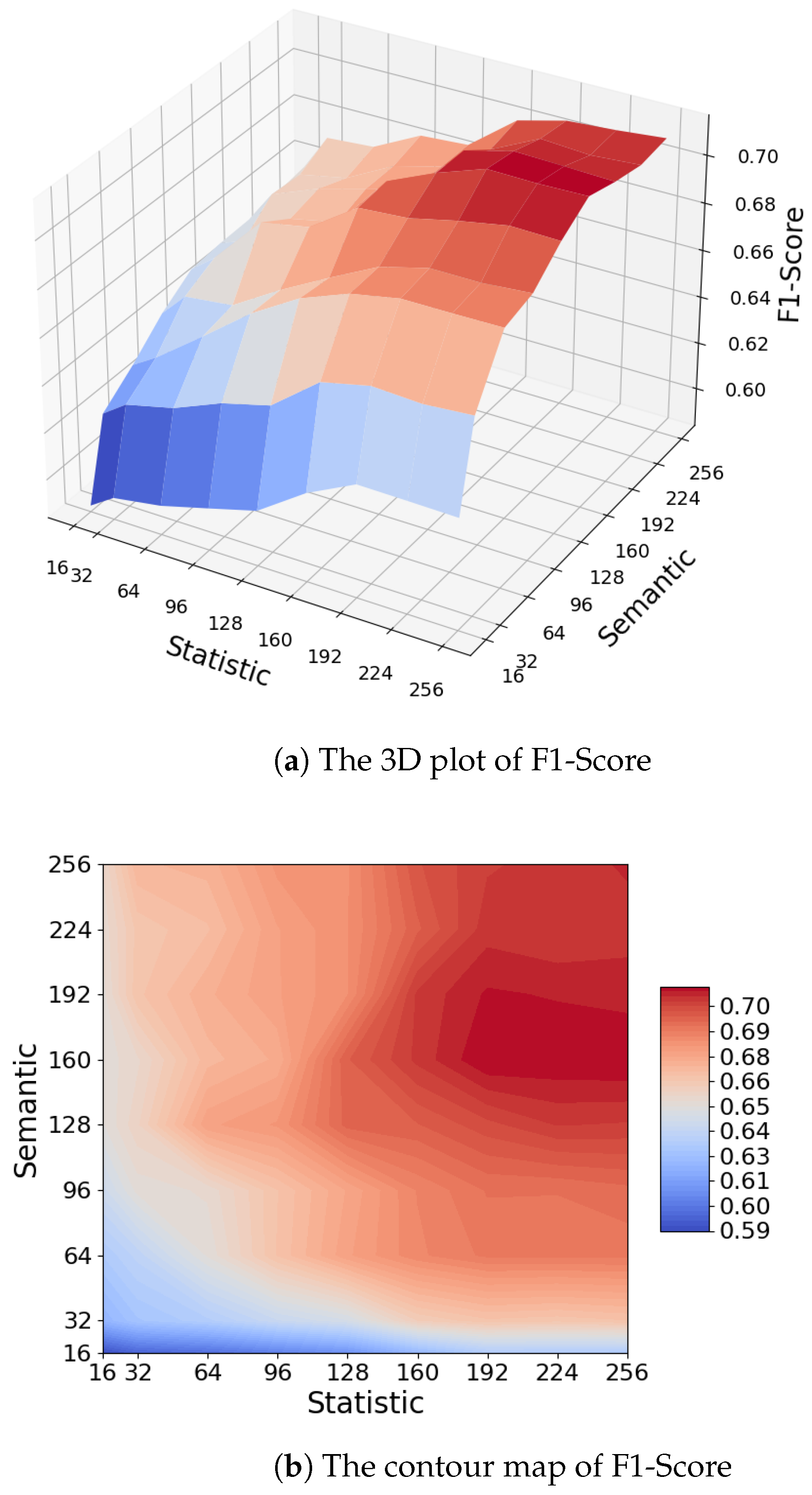
First, we make the two parts of the features to be generated using 16, 32, 64, 96, 128, 160, 192, 224 and 256 dimensions for all the data for the experiment. Figure 6a,b are the 3D plots of the F1-Score of the SDP-MTF using different combinations of dimensions and the corresponding contour schematics.

The closer the color to red in Figure 6 represents a higher F1-Score for that combination of dimensions, and the closer the color to blue indicates a lower F1-Score. We can see that the F1-Score of the model is low when the generated dimensions of both embeddings are low, and the F1-Score of the model starts to improve with the increase in feature dimensions, but when both embeddings are in high dimensions, the model dimensions gradually level off and no longer rise, and even have a tendency to fall. When the difference between the dimensions of the statistical feature dimension and the semantic feature is large, the model will tend to use the feature with a large dimension more for classification, resulting in the failure of the fusion feature, and the F1-Score tends to be closer to the performance of the feature alone. When the semantic feature dimension is low, Bi-LSTM cannot adequately capture the complexity of the utterance structure, leading to information loss, which affects the final task performance, so it is important to ensure the dimension of the semantic features, and it also restricts the statistical feature dimension not to differ too much from it. When the vector dimension is high, although the embedding vectors contain rich information, it may lead to overfitting, and also increase the computational complexity and memory requirements, which is the reason why the final F1-Score in Figure 6 has leveled off or even decreased. The model achieved the best average results at 160 dimensions for statistical features and 192 dimensions for semantic features, so we chose this parameter for model prediction in subsequent experiments and other research questions.

Next, we will explore the effect of each of the two feature lengths on the model’s effectiveness. Since the best results of the model were obtained when the statistical features were 160 dimensions and the semantic features were 192 dimensions, we will control the dimension change in a single variable in the next experiments while setting the other vector dimension to the above dimensions as a way to ensure the validity and reliability of the experiments. Figure 7 shows the performance of F1-Score of SDP-MTF on cross-project prediction when the dimension of a single vector is varied and the other vector is fixed to the nearest dimension, in which the red curve Statistic indicates the change in F1 value produced by the method when the dimension of the statistically based feature vectors is varied, in which case the dimension of the deep semantic vectors generated based on the Bi-LSTM is fixed at 192 dimensions; similarly, the gray Deep Semantic curve represents the change in the F1 value of the model caused by the change in the dimension of the semantic features, at which time the dimension of the statistical features is fixed to be unchanged at 160 dimensions. We can see that in all the experiments, the F1-Score of SDP-MTF is affected by the fusion feature dimensions, and the trend is that the F1-Score is lower in low dimensions, and as the vector dimensions increase, the F1-Score increases, and then tends to stabilize, and a smooth trend occurs after high dimensions. Among the two types of vectors, the model is more sensitive to changes in the dimension of the semantic features generated by Bi-LSTM, and the slopes of the folds are relatively larger.

Therefore, it can be concluded that the dimension size of the fused features has an effect on the final prediction results of the model, which is manifested in the fact that the F1-Score of the model firstly increases with the dimension of the two types of vectors, and then it tends to be stable or slightly fluctuates; therefore, the selection of appropriate generation dimension for the two types of vectors is necessary, and both types of vectors have an effect on the prediction results of the model. Meanwhile, the generating dimensions of 160 dimensions and 192 dimensions that we chose for the two features achieved the best results in our experiments, which also proved the effectiveness of our experiments.

RQ3 Results: The dimension of the fused features has an effect on the prediction effect of SDP-MTF, which is shown as follows: (1) when the dimension of the fused features is low, the prediction effect is low; (2) as the dimension of the fused features increases, the prediction effect appears to increase firstly and then stabilize; (3) when the dimension of the two vectors in the fused features has a large difference, the prediction effect tends to be the effect of the feature with larger dimension alone; (4) the model reaches the best result at 160 dimensions for the code statistical features and 192 dimensions for the semantic features, which is the final choice of the fusion feature dimension in our model.

5.4. Effectiveness of Multiple Transfer Learning

This subsection develops the ablation experiment for RQ4. This research question aims to investigate the effectiveness of multiple transfer learning methods for feature transfer and deep transfer learning, which refer to the method applied to statistical feature TCA+ and the method applied to deep adaptive neural networks with fused features, respectively.

Table 6. The F1-Score for SDP-MTF and algorithms using transfer learning alone.

Source Project	Target Project	SDP-MTF	SDP-UD	SDP-UT
Log4j	Camel	0.3988	0.2301	0.4058
Lucene		0.3969	0.3881	0.4382
Poi		0.3459	0.3186	0.4381
Xalan		0.3497	0.3454	0.3582
Xerces		0.4296	0.2826	0.4053
Camel	Log4j	0.7660	0.6233	0.6319
Lucene		0.7851	0.6281	0.6030
Poi		0.8016	0.5835	0.6565
Xalan		0.7593	0.5387	0.6854
Xerces		0.7852	0.6058	0.6775
Camel	Lucene	0.7466	0.5682	0.6596
Log4j		0.7424	0.6176	0.7127
Poi		0.7268	0.6104	0.6706
Xalan		0.7935	0.5702	0.6486
Xerces		0.7783	0.5271	0.6981
Camel	Poi	0.7396	0.5247	0.6937
Log4j		0.7561	0.4809	0.6456
Lucene		0.7796	0.5715	0.7233
Xalan		0.7966	0.5178	0.7005
Xerces		0.7555	0.4534	0.6393
Camel	Xalan	0.7592	0.6202	0.6666
Log4j		0.7822	0.5226	0.5857
Lucene		0.7984	0.5535	0.6464
Poi		0.7816	0.6076	0.6443
Xerces		0.7325	0.5653	0.5931
Camel	Xerces	0.7663	0.5016	0.6003
Log4j		0.7825	0.6029	0.5732
Lucene		0.7701	0.4671	0.602
Poi		0.7908	0.5766	0.6856
Xalan		0.7864	0.5699	0.5726
Avg		0.7061	0.6311	0.5990

shows the effect and F1-Score performance of the algorithmic model.

We set up the following ablation experiments: SDP-ND (Non-Domain Adaptation based), which uses fusion features generated by feature transfer but does not use a domain adaptation layer, SDP-NT (Non-TCA+ based), which is a method that uses the domain adaptation idea but does not use TCA+ for the code statistics features in the fusion features, and the original model SDP-MTF, i.e., the method that uses the multiple transfer learning idea.

From the table, we can learn that the SDP-MTF algorithm effectively improves the F1-Score using the transfer learning idea, which confirms the effectiveness of our proposed multiple transfer idea. In addition to this, the method SDP-NT without TCA+ outperforms the SDP-ND method without a domain adaptation layer. The SDP-NT method achieves an F1-Score of 0.6087, which is a 9.7% percentage difference compared to the SDP-MTF method; whereas, the SDP-ND method performs poorly in cross-project prediction due to the lack of a domain adaptation layer, with an average F1-Score of 0.5191, which is lower than the SDP-MTF method by 18.7%. This validates the need for transfer learning and the effectiveness of multiple transfer learning.

Figure 8 shows the stability effect of different algorithms. From left to right in the figure are SDP-MTF, SDP-ND without Domain Adaptation Layer and SDP-NT without TCA+. In terms of stability, SDP-UT has a similar IQR as SDP-MTF, with an IQR of 0.03 for the F1-Score, which indicates that both have similar generalization-ability and both have good stability. While the stability of SDP-UD is poorer, the IQR is 0.14, respectively, and the data fluctuate more. The comparison of the three suggests that multiple migration learning does not have a large impact on the fluctuation of the prediction effect.

We can infer the following information from this experiment: first, the idea of multiple transfer learning used by the method is effective, and our SDP-MTF method shows sufficient advantages, whether comparing algorithms that do not use the domain adaptation layer or methods that do not use feature transfer learning. Second, in terms of the stability of the algorithm, the use of multiple transfer learning does not cause large fluctuations in the predictors. Finally, the domain adaptation layer of deep transfer learning can effectively improve the prediction effect using semantic features and is an effective deep transfer method.

RQ4 Results: The idea of transfer learning method with deep adaptive neural network and multiple transfer learning with feature transfer that we use is effective, and under the same experimental conditions, SDP-MTF shows advantages in F1-Score over the algorithm without feature transfer and without domain adaptation layer, which improves the prediction.

6. Result Analysis and Discussion

6.1. Analysis and Comparison

From the above four RQs, we show the effectiveness of the model, the effectiveness of the fused features, the influence of feature dimensions on the prediction effect, and the effectiveness of the multiple transfer learning idea from multiple perspectives. In this subsection, we will explore the model effect in general and summarize the phenomena and conclusions observed in the above experiments.

Firstly, the model effectiveness. SDP-MTF shows different improvements in average F1-Score than the other six comparative baseline algorithms in all the 6-project, 30 cross-project pairs experiments. The use of fused features can fruitfully improve model prediction compared to algorithms that use statistical or semantic features of the code alone, as can be seen in the baseline algorithms BATM and CNN-THFL, which, as methods that also use two types of fused features, we can see that they are more effective than algorithms that use a particular type of feature alone, and they are ranked the second and the fourth out of all the algorithms. In addition, the poor performance of the DBN algorithm side-steps the fact that semantic features alone may not work very well for mining defective patterns, and that further work is needed to close the gap between projects or to include traditional features for information remediation. Finally, we also briefly assessed the stability of the individual algorithms, mainly by comparing the variance of the two metrics of each algorithm on all projects. The SDP-MTF algorithms show good stability on all F1-Score except for the Camel project. All these performances prove the effectiveness of our proposed SDP-MTF model.

This is followed by the evaluation of the SDP-MTF feature construction phase. In our experiments, it can be seen that the low cross-project prediction accuracy with the Camel project as the target project is directly related to the fact that the characteristics of the Camel project are significantly different from other projects and have a low defect rate. Differences in features between projects pose a significant challenge to cross-project defect prediction. Changes in feature distribution can lead to mismatches, which can degrade the model performance as the model may overfit the features of the source item or fail to generalize to the target item; therefore, in this paper, we abate the feature differences between items by two methods, TCA and DAN, as a way to provide a better feature space for migration learning. In order to test the effectiveness of feature-to-feature fusion, we designed RQ2 and RQ3 to test the model. We use Research Question 2 experiments to evaluate the effectiveness of fused features and to verify whether fusing code statistical features and semantic features can compensate for the problem of insufficient feature information mining. The experiments demonstrate that fused features have a higher prediction effect than using one type of feature alone. Moreover, the effect of SDP-DS using only semantic features is lower than that of SDP-CS, which also side by side confirms that a single type of feature and the use of deep features alone may not bring good results and that the introduction of code statistical features to complement the information from another perspective of the procedure is beneficial to the mining and correlation of defective patterns.

RQ3 explores the effect of the dimensionality of fusion features on the prediction effectiveness. The dimensionality of fusion features is determined by the dimensions of both statistical and semantic features. The dimensionality of a feature vector is closely related to its information representation capability, which represents how much information and intrinsic relationships can be captured by the vector. Longer feature vectors tend to capture more complex and detailed features, but at the same time, excessively long generating dimensions for feature vectors may also lead to problems such as model complexity, sparsity of high-dimensional space, and excessive computational overhead of the model. In our experiments, we first used multiple sets of generating dimensions to make the dimensions of two vectors change at the same time and record the model performance; after that, we searched for the point where the lengths of two vectors are most suitable, fixed the generating dimension of one vector, respectively, and changed the lengths of the other vector to record the model changes. The experimental results show that the dimension of the fused features will have a non-negligible impact on the final prediction of the model, and when the feature dimension is low, there will be a phenomenon of insufficient feature information capture leading to low model effect, while with the increase in the generation dimension, the model effect will first increase and then converge to a stable state. In the experiment of single generation length change, the semantic feature length change generated by the Bi-LSTM model is more likely to cause the change in the whole model effect, which is related to the characteristic that Bi-LSTM is not good at dealing with long sequence information. Therefore, finally, we choose the feature dimension of 352 dimensions of fused features (160 dimensions of statistical features and 192 dimensions of semantic features) as the criterion for the experiment.

RQ4 focuses on verifying the effectiveness of multiple migration learning. In our model, two modes of feature migration and deep adaptive neural network are used, corresponding to the code statistical features and the fused features incorporating the semantic features, and the two parts are used in combination to reduce the inter-item variance and improve the prediction results. The core idea of both means is to reduce the variability of features across items. TCA+-based feature migration focuses more on mapping the features of different items into a unified space to reduce the variance and achieve feature dimension alignment. Deep adaptive neural networks, on the other hand, focus more on the adaptive processing of source and target domain data through adaptive layers. This adaptive layer design makes the data distributions in the source and target domains closer to each other, thus improving the efficiency and effectiveness of data migration. From the experimental results, both of the means we used successfully improved the prediction effect.

Finally, we explore the similarities and differences between SDP-MTF and baseline algorithms. We have chosen six comparison algorithms, which can be divided into three categories according to the different use of features, namely NNFilter and TCA+ which use coded statistical features alone, DBN and AC-GAN which use semantic features alone, and CNN-THFL which uses a combination of coded statistical and semantic features. For the two algorithms of coded statistical features, NNFilter and TCA+ The difference is that the former focuses on instance migration, while the latter takes in feature migration, and in terms of effect TCA+ gives better results than NNFilter, which also inspired our algorithms and CNN-THFL. Algorithms DBN and AC-GAN, which use semantic features alone, both mine information from token sequences and ASTs, respectively, while AC-GAN employs the idea of adversarial learning for the latter step of migration, which improves the model effect and gives better results than DBN. The two algorithms CNN-THFL and BATM are the rare methods we found to combine two features. Compared with CNN-THFL, the biggest difference of our algorithm is the introduction of a deep adaptive neural network in the migration learning model of the fused features; while comparing with BATM, our algorithm uses multiple migration learning to weaken the item differences, which makes the model further improve the prediction effect.

6.2. Potential Risks and Future Prospects

We next discuss potential threats to our approach. Firstly, the construction factor, the representative algorithms in the controlled experiments used in this paper cannot be traced back to the source code, and thus methods reproduced according to the article’s introduction are used, and the implementation of these methods may not be exactly the same as that of the original authors. Especially in the methods involving deep learning CNN-THFL and adversarial learning AC-GAN and BATM, although this paper adopts the parameter settings recommended by the original authors, it is not possible to reproduce the experimental environment and algorithmic constructions completely, and thus there may be some bias in the prediction results. In addition, this paper adopts the F1 score index as a comprehensive evaluation index to evaluate the model and lacks the index evaluation index in the unbalanced scenario.

Next, are the internal factors. The method proposed in this paper does not do the treatment of imbalance, and there is no guarantee that the method will achieve the same effect for samples with imbalanced defects. At the same time, this paper uses the method of combining code statistical features with deep semantic features to make up for the problem of a single type of feature, but in terms of the fusion means, this section only uses $contact$ splicing operation and does not give enough consideration to other means of feature fusion, which may affect the model’s final prediction accuracy, and the use of different feature fusion methods to better combine the two types of features is a future. The use of different feature fusion methods and the better combination of the two types of features are the key perspectives for further mining of feature information.

Finally, there are external factors. This paper uses the PROMISE dataset as the experimental dataset, these datasets are written in Java language, the defects contained in these datasets may be with tendency, and these datasets are small in size, this paper can not guarantee that the model achieves the same effect on other languages written in a larger scale project.

Looking forward, in response to these challenges, we plan to test our model on samples written in various programming languages and apply it in more realistic, real-world scenarios [29,30]. Additionally, we aim to delve deeper into the relationship between various representations of deep semantic features and defect patterns. Exploring alternative representations such as control flow graphs and data flow diagrams could enhance prediction effect [31,32]. Moreover, while our current methodology concentrates on single-source cross-project software defect prediction, exploring multi-source scenarios represents a compelling direction for future research [33]. In addition, To ensure the reliability of AI-based defect prediction models, formal methods can be employed for rigorous verification. By applying formal methods, we can verify that AI models adhere to predefined specifications and perform consistently across different projects, thus ensuring accurate and reliable defect predictions [34,35]. Finally, how to introduce interpretable analyses into cross-project software defect prediction research and use the results of cross-project software defect prediction and these interpretable analyses to be extracted and transformed into something that testers can accept and recognize and use for deeper guidance on software security [36] is a theme that we will continue to focus on.

7. Conclusions

Cross-project software defect prediction addresses the cold start problem and early data scarcity in software defect prediction, representing a critical approach to software quality assurance. However, current methodologies predominantly grapple with two challenges: inadequate feature information mining and significant probabilistic distribution gaps between projects, leading to reduced effect. To tackle these issues, we propose the SDP-MTF method, which integrates feature fusion and composite transfer learning. By merging code statistical features with deep semantic features, we mine source code information from diverse perspectives, addressing the problem of incomplete feature information. Additionally, our approach employs a composite transfer learning strategy combining feature transfer based on TCA+ with DAN, effectively narrowing the gap between projects and concluding with defect prediction via the SVM classifier. We evaluated SDP-MTF on six projects from the PROMISE dataset, demonstrating its efficacy across various dimensions. The results show that SDP-MTF significantly outperforms six advanced baseline algorithms employing different feature methods, with an average improvement of 8% to 15.2% on the F1-Score. Future work will extend this research to real-world projects and explore multi-source cross-project defect prediction through further experimental studies.

References

1. Hall, T.; Beecham, S.; Bowes, D.; Gray, D.; Counsell, S. A Systematic Literature Review on Fault Prediction Performance in Software Engineering. IEEE Trans. Softw. Eng. 2012, 38, 1276–1304. [Google Scholar] [CrossRef]
2. Chen, X.; Wang, L.P.; Gu, Q.; Wang, Z.; Ni, C.; Liu, W.S.; Wang, Q.P. A Survey on Cross-Project Software Defect Prediction Methods. Jisuanji Xuebao Chin. J. Comput. 2018, 41, 254–274. [Google Scholar]
3. Briand, L.C.; Melo, W.L.; Wust, J. Assessing the applicability of fault-proneness models across object-oriented software projects. IEEE Trans. Softw. Eng. 2002, 28, 706–720. [Google Scholar] [CrossRef]
4. Nam, J.; Pan, S.J.; Kim, S. Transfer defect learning. In Proceedings of the 2013 35th International Conference on Software Engineering (ICSE), San Francisco, CA, USA, 18–26 May 2013; pp. 382–391. [Google Scholar]
5. Pan, S.J.; Tsang, I.W.; Kwok, J.T.; Yang, Q. Domain adaptation via transfer component analysis. IEEE Trans. Neural Netw. 2010, 22, 199–210. [Google Scholar] [CrossRef]
6. He, P.; Li, B.; Liu, X.; Chen, J.; Ma, Y. An empirical study on software defect prediction with a simplified metric set. Inf. Softw. Technol. 2015, 59, 170–190. [Google Scholar] [CrossRef]
7. Ni, C.; Chen, X.; Liu, W.; Gu, Q.; Huang, Q.; Li, N. Cross-project defect prediction method based on feature transfer and instance transfer. J. Softw. 2019, 30, 1308–1329. [Google Scholar]
8. Yao, Y.; Doretto, G. Boosting for transfer learning with multiple sources. In Proceedings of the 2010 IEEE Computer Society Conference on Computer Vision and Pattern Recognition, San Francisco, CA, USA, 13–18 June 2010; pp. 1855–1862. [Google Scholar]
9. Hosseini, S.; Turhan, B. A comparison of similarity based instance selection methods for cross project defect prediction. In Proceedings of the 36th Annual ACM Symposium on Applied Computing, Virtual Event, 22–26 March 2021; pp. 1455–1464. [Google Scholar]
10. Lei, T.; Xue, J.; Wang, Y.; Niu, Z.; Shi, Z.; Zhang, Y. WCM-WTrA: A Cross-Project Defect Prediction Method Based on Feature Selection and Distance-Weight Transfer Learning. Chin. J. Electron. 2022, 31, 354–366. [Google Scholar] [CrossRef]
11. Chen, D.; Li, B.; Zhou, C.; Zhu, X. Automatically identifying bug entities and relations for bug analysis. In Proceedings of the 2019 IEEE 1st International Workshop on Intelligent Bug Fixing (IBF), Hangzhou, China, 24 February 2019; pp. 39–43. [Google Scholar]
12. Wang, W.; Li, G.; Ma, B.; Xia, X.; Jin, Z. Detecting code clones with graph neural network and flow-augmented abstract syntax tree. In Proceedings of the 2020 IEEE 27th International Conference on Software Analysis, Evolution and Reengineering (SANER), London, ON, Canada, 18–21 February 2020; pp. 261–271. [Google Scholar]
13. Li, D.; Wong, W.E.; Jian, M.; Geng, Y.; Chau, M. Improving search-based automatic program repair with Neural Machine Translation. IEEE Access 2022, 10, 51167–51175. [Google Scholar] [CrossRef]
14. Wang, S.; Liu, T.; Tan, L. Automatically learning semantic features for defect prediction. In Proceedings of the 38th International Conference on Software Engineering, Austin, TX, USA, 14–22 May 2016; pp. 297–308. [Google Scholar]
15. Li, J.; He, P.; Zhu, J.; Lyu, M.R. Software defect prediction via convolutional neural network. In Proceedings of the 2017 IEEE International Conference on Software Quality, Reliability and Security (QRS), Prague, Czech Republic, 5–29 July 2017; pp. 318–328. [Google Scholar]
16. Qiu, S.; Lu, L.; Cai, Z.; Jiang, S. Cross-Project Defect Prediction via Transferable Deep Learning-Generated and Handcrafted Features. In Proceedings of the SEKE, Lisbon, Portugal, 10–12 July 2019; pp. 431–552. [Google Scholar]
17. Gupta, M.; Rajnish, K.; Bhattacharjee, V. Cognitive Complexity and Graph Convolutional Approach Over Control Flow Graph for Software Defect Prediction. IEEE Access 2022, 10, 108870–108894. [Google Scholar] [CrossRef]
18. Hamer, P.G.; Frewin, G.D. MH Halstead’s Software Science-a critical examination. In Proceedings of the 6th International Conference on Software Engineering, Tokyo, Japan, 13–16 September 1982; pp. 197–206. [Google Scholar]
19. Jureczko, M.; Madeyski, L. Towards identifying software project clusters with regard to defect prediction. In Proceedings of the 6th International Conference on Predictive Models in Software Engineering, Timişoara, Romania, 12–13 September 2010; pp. 1–10. [Google Scholar]
20. Vaswani, A.; Shazeer, N.; Parmar, N.; Uszkoreit, J.; Jones, L.; Gomez, A.N.; Kaiser, Ł.; Polosukhin, I. Attention is all you need. Adv. Neural Inf. Process. Syst. 2017, 30. [Google Scholar]
21. Long, M.; Cao, Y.; Wang, J.; Jordan, M. Learning transferable features with deep adaptation networks. In Proceedings of the 25th International Conference on Machine Learning (ICML), Lille, France, 6–11 July 2015; pp. 97–105. [Google Scholar]
22. Wang, J.; Chen, Y.; Hao, S.; Peng, X.; Hu, L. Deep learning for sensor-based activity recognition: A survey. Pattern Recognit. Lett. 2019, 119, 3–11, Deep Learning for Pattern Recognition. [Google Scholar] [CrossRef]
23. Gretton, A.; Borgwardt, K.M.; Rasch, M.J.; Schölkopf, B.; Smola, A. A kernel two-sample test. J. Mach. Learn. Res. 2012, 13, 723–773. [Google Scholar]
24. Belkin, M.; Niyogi, P.; Sindhwani, V. Manifold regularization: A geometric framework for learning from labeled and unlabeled examples. J. Mach. Learn. Res. 2006, 7, 2399–2434. [Google Scholar]
25. Turhan, B.; Menzies, T.; Bener, A.B.; Di Stefano, J. On the relative value of cross-company and within-company data for defect prediction. Empir. Softw. Eng. 2009, 14, 540–578. [Google Scholar] [CrossRef]
26. Wang, S.; Liu, T.; Nam, J.; Tan, L. Deep semantic feature learning for software defect prediction. IEEE Trans. Softw. Eng. 2018, 46, 1267–1293. [Google Scholar] [CrossRef]
27. Xing, Y.; Qian, X.; Guan, Y.; Zhang, S.; Zhao, M.; Lin, W. Cross-project Defect Prediction Method Using Adversarial Learning. J. Softw. 2022, 33, 2097–2112. [Google Scholar]
28. Jiang, S.; Zhang, J.; Guo, F.; Ouyang, T.; Li, J. Balanced Adversarial Tight Matching for Cross-Project Defect Prediction. IET Softw. 2024, 2024, 1561351. [Google Scholar] [CrossRef]
29. Tang, L.; Bao, L.; Xia, X.; Huang, Z. Neural SZZ algorithm. In Proceedings of the 2023 38th IEEE/ACM International Conference on Automated Software Engineering (ASE), Luxembourg, 11–15 September 2023; pp. 1024–1035. [Google Scholar]
30. Yang, Y.; Xia, X.; Lo, D.; Grundy, J. A survey on deep learning for software engineering. ACM Comput. Surv. 2022, 54, 1–73. [Google Scholar] [CrossRef]
31. Xu, J.; Wang, F.; Ai, J. Defect prediction with semantics and context features of codes based on graph representation learning. IEEE Trans. Reliab. 2020, 70, 613–625. [Google Scholar] [CrossRef]
32. Ni, C.; Wang, W.; Yang, K.; Xia, X.; Liu, K.; Lo, D. The best of both worlds: Integrating semantic features with expert features for defect prediction and localization. In Proceedings of the 30th ACM Joint European Software Engineering Conference and Symposium on the Foundations of Software Engineering, Singapore, 14–18 November 2022; pp. 672–683. [Google Scholar]
33. Ryu, D.; Baik, J. Effective multi-objective naïve Bayes learning for cross-project defect prediction. Appl. Soft Comput. 2016, 49, 1062–1077. [Google Scholar] [CrossRef]
34. Krichen, M.; Mihoub, A.; Alzahrani, M.Y.; Adoni, W.Y.H.; Nahhal, T. Are Formal Methods Applicable to Machine Learning and Artificial Intelligence? In Proceedings of the 2022 2nd International Conference of Smart Systems and Emerging Technologies (SMARTTECH), Riyadh, Saudi Arabia, 9–11 May 2022; pp. 48–53. [Google Scholar]
35. Raman, R.; Gupta, N.; Jeppu, Y. Framework for Formal Verification of Machine Learning Based Complex System-of-Systems. Insight 2023, 26, 91–102. [Google Scholar] [CrossRef]
36. Dam, H.K.; Tran, T.; Ghose, A. Explainable software analytics. In Proceedings of the 40th International Conference on Software Engineering: New Ideas and Emerging Results, Gothenburg, Sweden, 27 May–3 June 2018; pp. 53–56. [Google Scholar]
Figure 1. The framework of SDP-MTF.
Electronics 13 02439 g001
Figure 2. The framework of the feature generation phase.
Electronics 13 02439 g002
Figure 3. The schematic of DAN used in SDP-MTF.
Electronics 13 02439 g003
Figure 4. The stability of F1-Score of SDP-MTF and baseline algorithms on different target projects.
Electronics 13 02439 g004
Figure 5. The stability of F1-Score of SDP-MTF and comparison algorithms using feature alone on different target projects.
Electronics 13 02439 g005
Figure 6. The effect of feature dimensions on the F1-Score of the SDP-MTF.
Electronics 13 02439 g006
Figure 7. The mean F1-Score performance of SDP-MTF when using a single transformed feature dimension.
Electronics 13 02439 g007
Figure 8. The stability of F1-Score of algorithms for SDP-MTF and single transfer learning on different target projects.
Electronics 13 02439 g008