Automatic Classification of Defective Solar Panels in Electroluminescence Images Based on Random Connection Network

Abstract

Solar energy is an important renewable energy source, and the efficiency of solar panels is crucial. However, tiny cracks and dark spots, defects of panels, can significantly affect power generation performance. To solve the defect identification problem of solar panels, an intelligent electroluminescence (EL) image classification method based on a random network (RandomNet50) is proposed. The randomly connected network module is designed by combining dropout and feature reuse strategies. Feature reuse in random networks optimizes the network structure and improves the feature utilization efficiency. The network model uses geometric transformation and the deep convolution generative adversarial network (DCGAN) method to enhance few-shot EL images (400) with different states. The comparison experiment shows that the RandomNet50 has a good classification effect on the enhanced images. The accuracy of the CIFAR-10/EL dataset (96.15%/88.23%) is better than the residual and dense networks. The method has high classification accuracy and provides strong technical support in the field of solar cells.

1. Introduction

With the rapid development of society, global energy consumption has intensified, and environmental pollution caused by nonrenewable fossil energy has become increasingly severe. The demand for the development of clean energy is increasing, and new energy generation technology is increasingly sought after by countries worldwide [1]. Solar cells, as a new energy product, have become a popular photovoltaic (PV) market leader in recent years [2]. With the increase in photovoltaic installations, the demand for rapid evaluation of solar panel performance in the construction and operation of photovoltaic power stations has increased.

With the continuous advancement of technology, a variety of innovations have emerged in the field of solar cells to optimize the performance of silicon solar cells, including the methods of heterojunction with intrinsic thin layer (HIT) [3], tunnel oxide-passivated contact (TOPCon) [4], metal wrap through (MWT) [5], interdigitated back contact (IBC) [6], passive emitter and rear cell (PERC) [7], etc. Different types of silicon solar cells can produce electroluminescent images under appropriate test conditions to detect internal defects. These images can provide important information about the internal quality of the cell, helping manufacturers optimize the production process and improve the efficiency and reliability of the cell.

Defect areas can be quickly located by analyzing the brightness degree of each region in electroluminescence (EL) images [8]. The principle of EL technology involves applying a forward bias voltage to both ends of the silicon solar cell, leading to unbalanced carrier recombination and infrared light emission. The luminescence intensity distribution in the EL images corresponds to the presence of material defects of solar cells, indicating fewer/higher defects in higher intensity areas and lower intensity areas [9]. EL technology can detect both internal and external defects in solar cells and distinguish the types of defects. EL images can be efficiently captured using either charge-coupled device (CCD) cameras or professional shortwave infrared cameras, providing high-resolution imagery. This method of acquisition is characterized by its speed and has been widely implemented in both production settings and laboratory environments. The primary defects of solar cells include dark spots, cracks, scratches, etc. These problems may occur after the initial field operation or when the solar panels are affected by electrical and thermal stresses. Due to its low cost, high accuracy, and linearity, EL image detection of solar cell modules has become an effective detection method in the production of cell modules. Several defect-recognition techniques have been proposed for solar panels in recent years. EL imaging is widely used in defect and crack analysis. Ji et al. [10] proposed a method for measuring the electric field distribution and an image processing algorithm based on the EL effect. There are three main steps: spraying an epoxy coating mixed with ZnS, depositing a Cu electroluminescent powder on the insulator surface, obtaining photoluminescence images under different voltages, and determining the electric field distribution via the proposed image processing algorithm. Fioresi et al. [11] proposed a deep learning-based semantic segmentation model that identifies and segments defects in EL images of silicon PV cells, which utilizes a segmentation Deeplabv3 model with a ResNet50 backbone.

Deep learning methods, such as computer vision, automatic drive, and voice recognition, have gained considerable attention in various fields [12,13]. Along with open-source deep learning software frameworks (TensorFlow 2.6.2 [14] and PyTorch 2.0.0 [15]), an explosion in the availability of high-performance computing infrastructures (especially GPUs [16]), new network architectures [17], and training techniques [18] means that neural networks can be trained much deeper. The latest advances in deep learning techniques based on convolutional neural networks have led to significant progress in object localization and recognition under natural conditions, such as regions with convolutional neural network (R-CNN) features [19], spatial pyramid pooling networks [20], fast region convolutional neural networks [21], faster region CNN [22], single shot multibox detectors [23], you only look once [24], region-based fully convolutional networks (FCN) [25], and other extended variants of networks [26,27]. For example, an intelligent algorithm utilizing both a high-resolution network (HRNet) and self-fusion network (SeFNet) for automatic defect identification of PV modules using EL images has been proposed, demonstrating enhanced feature fusion and classification accuracy for superior defect recognition performance [28]. Korovin et al. [29] introduced SeMaCNN for the automatic detection, classification, and anomaly detection of EL images to assess solar cell quality, achieving 95.8% accuracy and a 92.5% F1 score for binary classification. Xie et al. [30] introduced an attention-based transfer learning approach with a class-aware domain discriminator to enhance the effect of knowledge transfer for defect detection in EL images, improving the F1 score by 0.2631, recall by 84.70%, and precision by 90.15%. Zhang et al. [31] proposed a novel lightweight high-performing model for automatic defect detection in PV cells of EL images, utilizing the neural architecture search and knowledge distillation for deploy ability, achieving 91.74% accuracy under online data augmentation.

Conventional image classification algorithms rely on the manual delineation of features, which is inefficient and requires researchers to sufficiently understand specific tasks [32]. The CNN proposed by researchers has overcome this bottleneck. However, convolutional neural networks pose another problem. Theoretically, if the depth or width of the network is increased during feature extraction, the extracted details and abstraction capability will be richer. Due to the mathematical properties of the backpropagation algorithm when updating the network weight, the problem of gradient explosion or gradient dispersion occurs when the layer quantity of the neural network increases. Traditional solutions, such as normalized initialization and batch normalization, solve the gradient problem but degrade network performance. Researchers have proposed a residual network to overcome the disadvantage of neural network performance degradation due to the increase in depth, inspired by the highway network. The integration of “shortcuts” and “skip connections” between the initial and subsequent layers enhances the flow of gradients during the training process, thereby enabling the successful training of deep CNNs. This is a key feature of the ResNet [33] architecture, which is illustrated in Figure 1a.

Inspired by the architecture of ResNet, researchers have developed densely connected convolutional networks (DenseNet) [34]. These networks employ a similar foundation of skip connections, as seen in ResNet. DenseNet has a more compact design with a significantly reduced number of parameters, as opposed to the hundreds or thousands of layers found in other networks. This streamlined approach enhances the flow of features and gradients, simplifying the training process. It also helps to mitigate overfitting and decreases computational requirements. The structure of DenseNet is shown in Figure 1b.

The feature reuse significantly improves the detection accuracy. Feng. et al. [35] introduced a fast segmentation network model called the feature reused network (FR-Net), which improves the detection of small defects and enhances real-time detection performance in the strip steel surface quality inspection process. In FR-Net, a feature fusion module is used to construct a feature reuse fusion bypass to improve the segmentation accuracy for small defects. Souaidi et al. [36] proposed an innovative SSD model, a densely connected single-shot multibox detector (DC-SSDNet), which is a DenseNet-based architecture that significantly improved the detection of small polyp regions, achieving an mAP of 93.96% and F1 score of 90.7%. Xie et al. [37] proposed a multiconnection pattern for a stochastic neural network, which defined the random network generator. Firstly, the network generator produces a general graph (based on the sense of graph theory). A set of nodes and edges connecting the nodes is generated without restricting the correspondence between the graph and the neural network (allowing the use of any general graph generator freely in graph theory). Once a graph is obtained, it is mapped to a computable neural network. Then, the classic random graph model is used to generate the random connection graphs of the network. Most state-of-the-art neural network models are hand-designed, ranging from simple chain models to structures with multiple paths. For example, the effectiveness of ResNet and DenseNet is largely attributed to their innovative network architectures.

To further explore the effect of feature reuse in the network, a random connection network is proposed, combining the idea of dropout and feature reuse. The feature reuse characteristic in random networks makes it possible that different random parameter settings determine the network’s structure and feature repetition rate. Higher random parameter settings result in deeper network models with a higher feature repetition rate, reducing error without adding many weights and biases. This paper proposed a method for classifying defective solar panels leveraging random connectivity. This method utilizes multiscale and multilevel object information to perform comprehensive image-to-image predictions, effectively identifying low-level edges, boundaries, and the contours of targets.

2. Materials and Methods

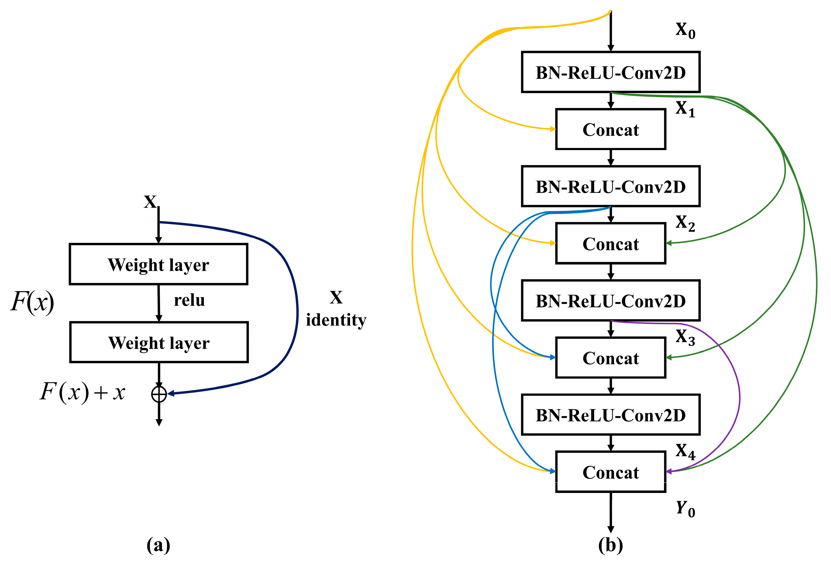
2.1. Proposed Model

An EL image classification method based on a random connection network is proposed. The network includes four random blocks, five convolutional layers, three pooling layers, one activation layer, and one fully connected layer. Batch normalization is added between the convolutional layer and the activation layer to speed up the training process, reducing the sensitivity to initialization and acting as a regularization function to avoid overfitting. The improved exponential linear unit (LeakyReLU) function is used for activation. The overall procedure of the proposed approach is illustrated in Figure 2.

The concepts of dropout and feature reuse are combined. In the network, the features of the current layer are randomly mapped to subsequent layers based on random rules. With feature reuse, features are repeatedly mapped from the front to the back layer; the network architecture contains dense connections, similar to the DenseNet framework. Additionally, the dropout technique is integrated. As a regularization method that randomly disconnects network connections to prevent overfitting, dropout optimizes the training process and enhances the depth of the network and the ability to extract features efficiently by using random skips. The fusion of high-level and low-level features contributes to a robust anti-overfitting capability, significantly improving the performance of the network.

The core module of the random connection network is random block $R$, whose skip rule includes skip length and times. The skip is realized in the same module. Batch normalization is added between the convolutional and activation layers to speed up the training process, reducing the sensitivity to initialization and avoiding overfitting. The inputs to each layer are affected by the parameters of all the preceding layers so that small changes in the network parameters amplify as the network deepens. In our network, the implement batch normalization ensured that the scale of the layer parameters has no effect of the backpropagation process, reducing the sensitivity to parameter initialization. By maintaining a stable distribution of inputs to nonlinearities during training, we prevented the optimizer from becoming trapped in saturated regimes, which accelerates the training process in turn. For activation, we utilized the Leaky Rectified Linear Unit (LeakyReLU) functions and applied L2 regularization to all layers to mitigate overfitting and enhance the model’s generalization ability. Additionally, dropout is incorporated in the fully connected (FC) layer to further improve the robustness of the network.

Four convolutional layers are set in the random block model, and the convolution kernel $R$ contains the quantity of skips $N$ and the length of skips $L$, as shown in Figure 3.

$$N=\{N\in N^{*}|N_{\mathrm{m}\mathrm{i}\mathrm{n}}<N<N_{\mathrm{m}\mathrm{a}\mathrm{x}}\}$$

(1)

$$L=\{L\in N^{*}|0<L<L_{\mathrm{m}\mathrm{a}\mathrm{x}}\}$$

(2)

where $N_{\mathrm{m}\mathrm{i}\mathrm{n}}=⌈\frac{n-i}{2}⌉$, $N_{\mathrm{m}\mathrm{a}\mathrm{x}}=n-i$, $L_{\mathrm{m}\mathrm{a}\mathrm{x}}=n-i$, $n$ is the total number of layers, $i$ is the current layer, and ⌈⌉ is the integral function up. Thus, the random matrix $R$ is mathematically represented as an upper triangular matrix.

Each current layer skips to the following layer through module $R$. In Figure 3, $Y_1$ skips to $Y_2$,$Y_3$, and $Y_5$; $Y_2$ skips to $Y_4$; and $Y_3$ skips to $Y_4$.

The random block output layer formula is as follows:

$$P=R^{T}Y+Q$$

(3)

$$\left[\begin{array}{c}{y}_2\\ y_3\\ \cdots \\ y_{n-1}\\ y_n\end{array}\right]=R^T\left[\begin{array}{c}f\left(y_1\right)\\ f\left(y_2\right)\\ \cdots \\ f\left(y_{n-2}\right)\\ f\left(y_{n-1}\right)\end{array}\right]+\left[\begin{array}{c}F(y_1,w_1)\\ F(y_2,w_2)\\ \cdots \\ F(y_{n-1},w_{n-1})\\ F(y_n,w_n)\end{array}\right]$$

(4)

where $P$ is the output matrix, $P=\left[\begin{array}{c}{y}_2\\ y_3\\ \cdots \\ y_{n-1}\\ y_n\end{array}\right]$. The matrix $R$ is generated by the random function $(N_{\mathrm{m}\mathrm{a}\mathrm{x}},N_{\mathrm{m}\mathrm{i}\mathrm{n}},L_{\mathrm{m}\mathrm{a}\mathrm{x}},L_{\mathrm{m}\mathrm{i}\mathrm{n}})$, the element has a value of 0 or 1, $R$ is a lower triangular matrix, $Y$ is the dimensional transformation matrix, and $Y=\left[\begin{array}{c}f\left(y_1\right)\\ f\left(y_2\right)\\ \cdots \\ f\left(y_{n-2}\right)\\ f\left(y_{n-1}\right)\end{array}\right]$. $Q$ is the convolution transformation matrix, $Q=\left[\begin{array}{c}F(y_1,w_1)\\ F(y_2,w_2)\\ \cdots \\ F(y_{n-1},w_{n-1})\\ F(y_n,w_n)\end{array}\right]$. The change in the dimension function is $f\left(x\right)$, the dimensional transformation function for skipping from $y_1$ to $y_2$ is $f\left(y_1\right)$, the convolutional layer transformation function is $F(y,w)$, and the output of the $w_1$ and $w_2$ operations is $F(x,(w_1,w_2\left)\right)$.

For example, in Figure 3, each output layer is expressed as:

$$\left[\begin{array}{c}{y}_2\\ y_3\\ y_4\\ y_5\end{array}\right]={\left[\begin{array}{cccc}1& 1& 0& 1\\ 0& 0& 1& 1\\ 0& 0& 1& 0\\ 0& 0& 0& 1\end{array}\right]}^T\left[\begin{array}{c}f\left(y_1\right)\\ f\left(y_2\right)\\ f\left(y_3\right)\\ f\left(y_4\right)\end{array}\right]+\left[\begin{array}{c}F(y_1,w_1)\\ F(y_2,w_2)\\ F(y_3,w_3)\\ F(y_4,w_4)\end{array}\right]$$

(5)

$$y_1=x$$

(6)

$$y_2=f\left(y_1\right)+F(y_1,w_1)$$

(7)

$$y_3=f\left(y_1\right)+F(y_2,w_2)$$

(8)

$$y_4=f\left(y_2\right)+f\left(y_3\right)+F(y_3,w_3)$$

(9)

$$y_5=f\left(y_1\right)+F(y_4,w_4)$$

(10)

2.2. Data Enhancement Model

A public EL image dataset consisting of 8-bit grayscale EL images of 300 × 300 pixels was used. It contains images of defects in different severity levels, such as images with dark spots, cracks, scratches, and defect-free images. A total of 200 defective and defect-free EL images were randomly selected from this dataset, respectively. To ensure the effectiveness of model training, we effectively partitioned the dataset, with 70% used for training and 30% for validation. Examples of EL images are shown in Figure 4.

Deep learning methods often achieve good results on datasets, while relying on large amounts of data and computing resources. When defect-free and defect images are trained in the same network, a serious convergence phenomenon occurs, affecting the recognition ability of the network. Therefore, under limited public datasets, it is necessary to expand the dataset through a series of data enhancement methods. The purpose of image enhancement is to enhance the information that is beneficial for pattern recognition, suppress the information that is unfavorable, and expand the feature differences between different objects in the image by processing part of the information in the image. Therefore, this paper adopts deep convolution generative adversarial networks (DCGANs) [38] to enhance the data quality.

The DCGAN model is mainly composed of a generative network and discriminant network. The generative network is used to generate a series of images for the discriminant network. The discriminant network mainly identifies the real image and a series of generated images from the generative network and discriminates the real image as “1”/“0”. Then, the generative network also adjusts itself through the results of the discriminant network, generating more similar images to the real image for deceiving the discriminant network. In this way, the generation level and discrimination level of the two networks are finally balanced through continuous mutual optimization. After reaching this equilibrium state, the process of extracting a large quantity of images from the generative network is used to enhance the ground truth image dataset, forming an enhancement strategy in data augmentation. The principle is that the generated composite image has a high degree of realism, and it is actually indistinguishable from real data samples when evaluated by a discriminative trained network.

The DCGAN structure mainly includes the generator network on the left and the discriminator network on the right, which has four DeConv and Conv layers, respectively. The structure of DCGAN is shown in Figure 5.

3. Experiments

3.1. Experimental Configuration

The programming project was developed using Python 3.8 in the PyCharm 2022.3 Integrated Development Environment (IDE). TensorFlow2x is the primary framework for software implementation launched by Google. Combining an NVIDIA graphics card, CUDA, and a GPU provided a platform for parallel computing, which improves the calculation speed.

3.2. Data Enhancement

There is a serious phenomenon of image convergence between defect-free images and defective images in the same network when the original dataset is used for network training, which affects the diversity of defect images, without reflecting good generalization performance by the classification model. To overcome the challenges of classification and imbalance of neural network data and avoid biased learning, augmenting the training dataset is a critical step in enhancing the model’s performance and robustness. Image augmentation is achieved by artificially generating training images. Processing can be performed through various processing methods or combinations, such as random rotation, shift, clipping, and flipping. By increasing the number of datasets, the quality of the datasets should also be enhanced. To address these limitations, we employed a geometric transformation technique to augment the dataset. Additionally, the DCGAN was leveraged to enhance the quality of the data. This dual approach expands the dataset and improves the richness or diversity of the data, which are essential for training robust and high-performing deep learning models. A portion of the image after data enhancement is shown in Figure 6.

3.3. Evaluation Indicator

The architecture of the deep random connection network is shown in

Table 1. The structure of the feature extraction network.

Input Name	Activations
Input layer	224 × 224 × 3
Convolution	7 × 7, 64, /2
Batch normalization	112 × 112, 64
Max pooling	56 × 56, 64
Block1	$\left[\begin{array}{c}1\times 1,\\ 3\times 3,\\ 3\times 3,\\ 1\times 1,\end{array}\begin{array}{c}64\\ 64\\ 64\\ 256\end{array}\right]\times 2$
Block2	$\left[\begin{array}{c}1\times 1,\\ 3\times 3,\\ 3\times 3,\\ 1\times 1,\end{array}\begin{array}{c}128\\ 128\\ 128\\ 516\end{array}\right]\times 4$
Block3	$\left[\begin{array}{c}1\times 1,\\ 3\times 3,\\ 3\times 3,\\ 1\times 1,\end{array}\begin{array}{c}256\\ 256\\ 256\\ 1024\end{array}\right]\times 4$
Block4	$\left[\begin{array}{c}1\times 1,\\ 3\times 3,\\ 3\times 3,\\ 1\times 1,\end{array}\begin{array}{c}512\\ 512\\ 512\\ 2048\end{array}\right]\times 2$

.

The hyperparameters of the deep random connection network are selected as follows: the batch size is 32 and the initial learning rate is 0.001; when the loss value is unchanged, the learning rate is reduced to the original 0.1, the loss function is binary cross-entropy, the activation function is sigmoid, and the LeakyReLU and Adam optimizers are used to optimize the model.

The loss function binary cross-entropy is used to evaluate the gap between the input and output, as shown in (12).

$$Loss=-\frac{1}{outputsize}\sum _{i=1}^{outputsize}{y}_i\cdot log{\widehat{y}}_i+(1-y_i)\cdot log(1-{\widehat{y}}_i)$$

(11)

The activation function in this work adopted the sigmoid function and LeakyReLU function, which are shown in (13) and (14), respectively.

$$Sigmoid=\frac{1}{1+{exp}^{-x}}$$

(12)

$$LeakyReLU=\left\{\begin{array}{ccc}ax& ,& x>0\\ x& ,& x\le 0\end{array}\right.$$

(13)

The optimization function in this work adopts adaptive moment estimation (Adam), a variant of the gradient descent method, to update the weight of the neural network, and the default values are used.

$$m_t={\beta }_1{m}_{t-1}+(1-{\beta }_1)g_t$$

(14)

$$v_t={\beta }_2{v}_{t-1}+(1-{\beta }_2)g_t^2$$

(15)

$${\widehat{m}}_t=\frac{m_t}{1-{\beta }_1^t}$$

(16)

$${\widehat{v}}_t=\frac{v_t}{1-{\beta }_2}$$

(17)

$${\theta }_{t+1}={\theta }_t-\frac{\eta }{\sqrt{{\widehat{v}}_t}+\epsilon }{\widehat{m}}_t$$

(18)

where $\eta =0.001$, ${\beta }_1=0.09$, ${\beta }_2=0.009$, $\epsilon =10^{-8}$, $\eta$ is the learning rate, ${\beta }_1$ and ${\beta }_2$ are numbers close to 1, and $g_t$ is the gradient. ${\widehat{m}}_t$ and ${\widehat{v}}_t$ are used for deviation correction, ${\theta }_t$ is used for parameter update, and $\epsilon$ is used to prevent division by 0.

3.4. Evaluation Criteria

For binary classification, the accuracy is the ratio of correctly predicted observations to the total number of events. True values are correctly predicted observations.

$$Accuracy=\frac{TP+TN}{TP+TN+FP+FN}$$

(19)

where $TP$ represents true positive values, $FP$ represents false positive values, $TN$ represents true negative values, and $FN$ represents false negative values.

3.5. Results Analysis and Discussion

The experiments include three parts: (1) Five types of traditional conventional CNN models, classifier 1 [39], classifier 2 [40], and the developed random network are used for model validation on the CIFAR-10 dataset. (2) Based on section (1), two models with high accuracy are selected and compared with developed random network models on the EL dataset by using the data enhancement method. (3) Influence on random networks with different network structures.

We chose a 50-layer network structure (RandomNet50) from the common network models (18, 34, 50, 101, 152, etc.). After entering the image data, the convolutional layer, batch normalization layer, activation layer, and maximum pooling layer in the RandomNet50 structure are first passed, followed by four random block modules and then passed through the global average pooling and fully connected layers.

To compare the performance of the models, we selected several commonly used models and the proposed RandomNet50 model for testing on the CIFAR-10 dataset. RandomNet50 was compared with several common classification models, AlexNet, VGG11, VGG19, ResNet50, classifier 1 [39], classifier 2 [40], and DenseNet50, as shown in Figure 7.

As shown in Figure 7, the accuracy of the AlexNet network is low, and the accuracy of the VGG11 and VGG19 networks is 92.61% and 93.65%, respectively. The accuracy of the ResNet50 network is almost the same as that of the DenseNet50 network and reaches 95.48%. The AlexNet network is highly sensitive to changes in the corresponding parameters. When AlexNet was originally proposed, the input images from the dataset had dimensions of 227 × 227, and we used the CIFAR-10 dataset with an image resolution of 32 × 32. Then, we modified the size of the first convolutional layer’s kernel to 3 × 3 and reduced the network’s pooling value. These modifications were necessary to adapt the AlexNet architecture to the new dataset. We found that increasing the number of training epochs had a significant impact on the accuracy of the network. After 200 training epochs, the accuracy reached 78.81%. However, the parameters of the DenseNet50 network are much smaller than the RenNet50 network. The accuracy of the RandomNet50 network is 0.67% higher than the ResNet50 network, and the parameters of the RandomNet50 network are fewer than those of ResNet50. This shows that a neural network is not necessarily a hierarchical structure. A layer in the network can depend not only on the features of the immediate upper layer but also on the features learned by the earlier layer. The results show that the accuracy of the RandomNet50 network is superior to AlexNet, VGG11, VGG19, ResNet50, and DenseNet50 on the CIFAR-10 dataset.

Through the comparison of previous experiments, three models with higher accuracy were selected for training on the EL dataset, and the performance of the results was observed. Figure 8 shows each method’s accuracy and loss curve from

Table 2. Comparisons of the classification results on the EL dataset.

Algorithm	Accuracy	Loss	Parameters
RandomNet50	88.23%	0.34	15.2 × 106
ResNet50	83.15%	0.41	21.3 × 106
DenseNet50	87.46%	0.35	7.0 × 106

. The RandomNet50 network achieves high accuracy in EL image recognition, which is 0.77% greater than the DenseNet50 network and 5.08% greater than that of the ResNet50 network. The network structure will lead to new breakthroughs when different network structures are obtained through random network models in the same space with reduced constraints.

The loss of the RandomNet50 network in EL image recognition is close to the DenseNet50 network and 0.07 lower than the ResNet50 network. Moreover, interference and noise in the image background can lead to a high loss value of the network. We used the EL dataset with a high gray value in the background. Under EL imaging, defects appear black, and the noise interference in the image background is relatively high. Overlearning the background noise interference affects the relationship between the real input and output. Figure 8 also shows that the loss of the RandomNet50 network is very high at the beginning and decreases relatively quickly.

The 50-layer network is composed of four convolution blocks. The conventional convolution block is composed of three convolution layers, and the random block can be applied to the third layer or above. Therefore, a 50-layer network was selected, and the influence of different convolution blocks on network performance is discussed. For the combination of four layers of convolution blocks, the numbers of convolution layers contained in the convolution blocks are [2,4,4,2], [2,4,5,2], and [4,3,3,4] (see

Table 3. Different network structures of RandomNet50.

Block Name	Activations-1	Activations-2	Activations-3
Block1	$\left[\begin{array}{c}1\times 1,\\ 3\times 3,\\ 3\times 3,\\ 1\times 1,\end{array}\begin{array}{c}64\\ 64\\ 64\\ 256\end{array}\right]\times 2$	$\left[\begin{array}{c}1\times 1,\\ 3\times 3,\\ 1\times 1,\end{array}\begin{array}{c}64\\ 64\\ 256\end{array}\right]\times 2$	$\left[\begin{array}{c}1\times 1,\\ 3\times 3,\\ 1\times 1,\end{array}\begin{array}{c}64\\ 64\\ 256\end{array}\right]\times 4$
Block2	$\left[\begin{array}{c}1\times 1,\\ 3\times 3,\\ 3\times 3,\\ 1\times 1,\end{array}\begin{array}{c}128\\ 128\\ 128\\ 512\end{array}\right]\times 4$	$\left[\begin{array}{c}1\times 1,\\ 3\times 3,\\ 3\times 3,\\ 1\times 1,\end{array}\begin{array}{c}128\\ 128\\ 128\\ 512\end{array}\right]\times 4$	$\left[\begin{array}{c}1\times 1,\\ 3\times 3,\\ 3\times 3,\\ 1\times 1,\end{array}\begin{array}{c}128\\ 128\\ 128\\ 512\end{array}\right]\times 3$
Block3	$\left[\begin{array}{c}1\times 1,\\ 3\times 3,\\ 3\times 3,\\ 1\times 1,\end{array}\begin{array}{c}256\\ 256\\ 256\\ 1024\end{array}\right]\times 4$	$\left[\begin{array}{c}1\times 1,\\ 3\times 3,\\ 3\times 3,\\ 1\times 1,\end{array}\begin{array}{c}256\\ 256\\ 256\\ 1024\end{array}\right]\times 5$	$\left[\begin{array}{c}1\times 1,\\ 3\times 3,\\ 3\times 3,\\ 1\times 1,\end{array}\begin{array}{c}256\\ 256\\ 256\\ 1024\end{array}\right]\times 3$
Block4	$\left[\begin{array}{c}1\times 1,\\ 3\times 3,\\ 3\times 3,\\ 1\times 1,\end{array}\begin{array}{c}512\\ 512\\ 512\\ 2048\end{array}\right]\times 2$	$\left[\begin{array}{c}1\times 1,\\ 3\times 3,\\ 1\times 1,\end{array}\begin{array}{c}512\\ 512\\ 2048\end{array}\right]\times 2$	$\left[\begin{array}{c}1\times 1,\\ 3\times 3,\\ 1\times 1,\end{array}\begin{array}{c}512\\ 512\\ 2048\end{array}\right]\times 4$

).

Table 4. Comparisons of the three structures on the EL dataset.

Structure	Accuracy
Activations-1	88.23%
Activations-2	88.15%
Activations-3	88.06%

shows that the three network structures have little impact on the network, and the accuracy is almost the same, showing the stable and robust nature of the network structure. Moreover, it can be concluded that random blocks can be inserted into the middle part of the neural network structure, which can improve the accuracy and stability of the network.

To further demonstrate the performance superiority of the model, we compared it with studies using the same dataset. The comparison results are shown in

Table 5. Comparison results with existing methods.

Resources	Methods	Accuracy	Sample Size
[41]	SVM (KAZE/VGG features)	82.44%	2624
[41]	CNN (Transfer learning)	88.42%	2624
[42]	CNN	93.02%	2624
[28]	SeF-HRNet	94.90%	2624
Ours	RandomNet50	88.23%	400

. The proposed method achieved 88.23% accuracy, which is 5.79% higher than that of the SVM method and almost the same as that of the CNN method under resource-constrained conditions, specifically with a limited dataset and a fixed number of training epochs of 200.

4. Conclusions and Future Work

The proposed new model (RandomNet50) integrates dropout and feature reuse strategies to construct an adaptable and computationally efficient structural framework. Data enhancement is used to process EL images in small sample scenes. The training and testing results on defective solar panel classification show that RandomNet50 is better than other test networks, and the accuracy is 88.23%, higher than ResNet50 and DenseNet50 (5.08% and 0.77%, respectively). The proposed method RandomNet50 had the highest accuracy (96.15%) compared with the accuracy of AlexNet, VGG11, VGG19, ResNet50, and DenseNet50 on the CIFAR-10 dataset. The results also showed that ResNet50 had a slight advantage over DenseNet50, achieving an accuracy of 95.48%. It is suitable for automatically classifying and detecting defective solar panels in EL images and has high robustness and generalizability.

We will continue to focus on improving the performance of our algorithms, including increasing the speed of defect detection and reducing the number of parameters in the network, while expanding the ability to identify different types of defects. At the application level, we plan to apply this method to video detection fields such as automatic detection and intelligent monitoring, in order to solve practical engineering problems.

References

1. Zhu, H.; Yan, W.; Liu, Y.; Hu, D.; Tu, Y.; Huang, Z.; Tan, X. Design investigation on 100 μm-thickness thin silicon PERC solar cells with assistance of machine learning. Mater. Sci. Semicond. Process. 2022, 137, 106198. [Google Scholar] [CrossRef]
2. Li, P.; Cao, Q.; Li, J.; Wang, Y.; Pei, G.; Gao, C.; Zhao, H.; Liu, X. Effect of regenerator on the direct steam generation solar power system characterized by prolonged thermal storage and stable power conversion. Renew. Energy 2020, 159, 1099–1116. [Google Scholar] [CrossRef]
3. Dao, V.A.; Kim, S.; Lee, Y.; Kim, S.; Park, J.; Ahn, S.; Yi, J. High-efficiency heterojunction with intrinsic thin-layer solar cells: A review. Curr. Photovolt. Res. 2013, 1, 73–81. [Google Scholar]
4. Feldmann, F.; Bivour, M.; Reichel, C.; Steinkemper, H.; Hermle, M.; Glunz, S.W. Tunnel oxide passivated contacts as an alternative to partial rear contacts. Sol. Energy Mater. Sol. Cells 2014, 131, 46–50. [Google Scholar] [CrossRef]
5. Clement, F.; Menkoe, M.; Kubera, T.; Harmel, C.; Hoenig, R.; Wolke, W.; Wirth, H.; Biro, D.; Preu, R. Industrially feasible multi-crystalline metal wrap through (MWT) silicon solar cells exceeding 16% efficiency. Sol. Energy Mater. Sol. Cells 2009, 93, 1051–1055. [Google Scholar] [CrossRef]
6. Verlinden, P. Backside-contact silicon solar cells with improved efficiency for the ’96 world solar challenge. Proc. 15th EU-PVSEC 1997. Available online: https://cir.nii.ac.jp/crid/1570854176739872768 (accessed on 18 June 2024).
7. Dehzangi, A.; Larki, F.; Majlis, B.Y.; Naseri, M.G.; Navasery, M.; Abdullah, A.M.; Hutagalung, S.D.; Hamid, N.A.; Noor, M.M.; Vakilian, M. Impact of KOH etching on nanostructure fabricated by local anodic oxidation method. Int. J. Electrochem. Sci. 2013, 8, 8084–8096. [Google Scholar] [CrossRef]
8. Rajput, A.S.; Ho, J.W.; Zhang, Y.; Nalluri, S.; Aberle, A.G. Quantitative estimation of electrical performance parameters of individual solar cells in silicon photovoltaic modules using electroluminescence imaging. Sol. Energy 2018, 173, 201–208. [Google Scholar] [CrossRef]
9. Karimi, A.M.; Fada, J.S.; Hossain, M.A.; Yang, S.; Peshek, T.J.; Braid, J.L.; French, R.H. Automated pipeline for photovoltaic module electroluminescence image processing and degradation feature classification. IEEE J. Photovolt. 2019, 9, 1324–1335. [Google Scholar] [CrossRef]
10. Ji, S.; Jia, Y.; Yang, X.; Liu, Z.; Zhu, L. A method for measuring electric field distribution along insulator surfaces based on electroluminescence effect and its image processing algorithm. IEEE Trans. Dielectr. Electr. Insul. 2022, 29, 939–947. [Google Scholar] [CrossRef]
11. Fioresi, J.; Colvin, D.J.; Frota, R.; Gupta, R.; Li, M.; Seigneur, H.P.; Vyas, S.; Oliveira, S.; Shah, M.; Davis, K.O. Automated defect detection and localization in photovoltaic cells using semantic segmentation of electroluminescence images. IEEE J. Photovolt. 2021, 12, 53–61. [Google Scholar] [CrossRef]
12. LeCun, Y.; Bengio, Y.; Hinton, G. Deep learning. Nature 2015, 521, 436–444. [Google Scholar] [CrossRef]
13. Krizhevsky, A.; Sutskever, I.; Hinton, G.E. ImageNet classification with deep convolutional neural networks. Commun. ACM 2017, 60, 84–90. [Google Scholar] [CrossRef]
14. Abadi, M.; Agarwal, A.; Barham, P.; Brevdo, E.; Chen, Z.; Citro, C.; Corrado, G.S.; Davis, A.; Dean, J.; Devin, M. Tensorflow: Large-scale machine learning on heterogeneous distributed systems. arXiv 2016, arXiv:1603.04467. [Google Scholar] [CrossRef]
15. Paszke, A.; Gross, S.; Massa, F.; Lerer, A.; Bradbury, J.; Chanan, G.; Killeen, T.; Lin, Z.; Gimelshein, N.; Antiga, L. Pytorch: An imperative style, high-performance deep learning library. arXiv 2019, arXiv:1912.0170332. [Google Scholar] [CrossRef]
16. Chetlur, S.; Woolley, C.; Vandermersch, P.; Cohen, J.; Tran, J.; Catanzaro, B.; Shelhamer, E. cudnn: Efficient primitives for deep learning. arXiv 2014, arXiv:1410.0759. [Google Scholar] [CrossRef]
17. Zeng, N.; Wang, Z.; Zineddin, B.; Li, Y.; Du, M.; Xiao, L.; Liu, X.; Young, T. Image-based quantitative analysis of gold immunochromatographic strip via cellular neural network approach. IEEE Trans. Med. Imaging 2014, 33, 1129–1136. [Google Scholar] [CrossRef]
18. Ioffe, S.; Szegedy, C. Batch normalization: Accelerating deep network training by reducing internal covariate shift. In Proceedings of the International Conference on Machine Learning, Lille, France, 6–11 July 2015; pp. 448–456. [Google Scholar]
19. Girshick, R.; Donahue, J.; Darrell, T.; Malik, J. Rich feature hierarchies for accurate object detection and semantic segmentation. In Proceedings of the IEEE Conference on Computer Vision and Pattern Recognition, Columbus, OH, USA, 23–28 June 2014; pp. 580–587. [Google Scholar]
20. He, K.; Zhang, X.; Ren, S.; Sun, J. Spatial pyramid pooling in deep convolutional networks for visual recognition. IEEE Trans. Pattern Anal. Mach. Intell. 2015, 37, 1904–1916. [Google Scholar] [CrossRef]
21. Girshick, R. Fast r-cnn. In Proceedings of the IEEE International Conference on Computer Vision, Santiago, Chile, 7–13 December 2015; pp. 1440–1448. [Google Scholar]
22. Ren, S.; He, K.; Girshick, R.; Sun, J. Faster r-cnn: Towards real-time object detection with region proposal networks. IEEE Trans. Pattern Anal. Mach. Intell. 2015, 39, 1137–1149. [Google Scholar] [CrossRef]
23. Liu, W.; Anguelov, D.; Erhan, D.; Szegedy, C.; Reed, S.; Fu, C.-Y.; Berg, A.C. Ssd: Single shot multibox detector. In Proceedings of the Computer Vision–ECCV 2016: 14th European Conference, Amsterdam, The Netherlands, 11–14 October 2016; pp. 21–37. [Google Scholar]
24. Redmon, J.; Divvala, S.; Girshick, R.; Farhadi, A. You only look once: Unified, real-time object detection. In Proceedings of the IEEE Conference on Computer Vision and Pattern Recognition, Las Vegas, NV, USA, 27–30 June 2016; pp. 779–788. [Google Scholar]
25. Dai, J.; Li, Y.; He, K.; Sun, J. R-fcn: Object detection via region-based fully convolutional networks. arXiv 2016, arXiv:1605.06409v3. [Google Scholar] [CrossRef]
26. Cai, Z.; Vasconcelos, N. Cascade r-cnn: Delving into high quality object detection. In Proceedings of the IEEE conference on computer vision and pattern recognition, Salt Lake City, UT, USA, 18–23 June 2018; pp. 6154–6162. [Google Scholar]
27. Hussain, T.; Hussain, M.; Al-Aqrabi, H.; Alsboui, T.; Hill, R. A review on defect detection of electroluminescence-based photovoltaic cell surface images using computer vision. Energies 2023, 16, 4012. [Google Scholar] [CrossRef]
28. Zhao, X.; Song, C.; Zhang, H.; Sun, X.; Zhao, J. HRNet-based automatic identification of photovoltaic module defects using electroluminescence images. Energy 2023, 267, 126605. [Google Scholar] [CrossRef]
29. Korovin, A.; Vasilev, A.; Egorov, F.; Saykin, D.; Terukov, E.; Shakhray, I.; Zhukov, L.; Budennyy, S. Anomaly detection in electroluminescence images of heterojunction solar cells. Sol. Energy 2023, 259, 130–136. [Google Scholar] [CrossRef]
30. Xie, X.; Lai, G.; You, M.; Liang, J.; Leng, B. Effective transfer learning of defect detection for photovoltaic module cells in electroluminescence images. Sol. Energy 2023, 250, 312–323. [Google Scholar] [CrossRef]
31. Zhang, J.; Chen, X.; Wei, H.; Zhang, K. A lightweight network for photovoltaic cell defect detection in electroluminescence images based on neural architecture search and knowledge distillation. Appl. Energy 2024, 355, 122184. [Google Scholar] [CrossRef]
32. Zhou, W.; Wang, H.; Wan, Z. Ore image classification based on improved CNN. Comput. Electr. Eng. 2022, 99, 107819. [Google Scholar] [CrossRef]
33. He, K.; Zhang, X.; Ren, S.; Sun, J. Deep residual learning for image recognition. In Proceedings of the IEEE Conference on Computer Vision and Pattern Recognition, Las Vegas, NV, USA, 27–30 June 2016; pp. 770–778. [Google Scholar]
34. Huang, G.; Liu, Z.; Van Der Maaten, L.; Weinberger, K.Q. Densely connected convolutional networks. In Proceedings of the IEEE Conference on Computer Vision and Pattern Recognition, Honolulu, HI, USA, 21–26 July 2017; pp. 4700–4708. [Google Scholar]
35. Feng, Q.; Li, F.; Li, H.; Liu, X.; Fei, J.; Xu, S.; Lu, C.; Yang, Q. Feature reused network: A fast segmentation network model for strip steel surfaces defects based on feature reused. Vis. Comput. 2024, 40, 3633–3648. [Google Scholar] [CrossRef]
36. Souaidi, M.; Lafraxo, S.; Kerkaou, Z.; El Ansari, M.; Koutti, L. A multiscale polyp detection approach for gi tract images based on improved densenet and single-shot multibox detector. Diagnostics 2023, 13, 733. [Google Scholar] [CrossRef]
37. Xie, S.; Kirillov, A.; Girshick, R.; He, K. Exploring randomly wired neural networks for image recognition. In Proceedings of the IEEE/CVF International Conference on Computer Vision, Seoul, Republic of Korea, 27 October–2 November 2019; pp. 1284–1293. [Google Scholar]
38. Radford, A.; Metz, L.; Chintala, S. Unsupervised representation learning with deep convolutional generative adversarial networks. arXiv 2015, arXiv:1511.06434. [Google Scholar] [CrossRef]
39. Sun, W.; Zhang, X.; He, X. Lightweight image classifier using dilated and depthwise separable convolutions. J. Cloud Comput. 2020, 9, 55. [Google Scholar] [CrossRef]
40. Sharma, A.K.; Rana, A.; Kim, K.K. Lightweight image classifier for CIFAR-10. J. Sens. Sci. Technol. 2021, 30, 286–289. [Google Scholar] [CrossRef]
41. Deitsch, S.; Christlein, V.; Berger, S.; Buerhop-Lutz, C.; Maier, A.; Gallwitz, F.; Riess, C. Automatic classification of defective photovoltaic module cells in electroluminescence images. Sol. Energy 2019, 185, 455–468. [Google Scholar] [CrossRef]
42. Akram, M.W.; Li, G.; Jin, Y.; Chen, X.; Zhu, C.; Zhao, X.; Khaliq, A.; Faheem, M.; Ahmad, A. CNN based automatic detection of photovoltaic cell defects in electroluminescence images. Energy 2019, 189, 116319. [Google Scholar] [CrossRef]
Figure 1. The samples of the network model: (a) ResNet block; and (b) DenseNet block.
Electronics 13 02429 g001
Figure 2. Schematic of the overall process structure of the random network.
Electronics 13 02429 g002
Figure 3. Random block structure of four convolutional layers. Notes: the matrix R is an example of Formula (5), generated by a random function.
Electronics 13 02429 g003
Figure 4. The partial samples of the EL images dataset: (a) dark spots; (b) cracks; (c) scratches; and (d) defect-free.
Electronics 13 02429 g004
Figure 5. The deep convolution generative adversarial network structure. Note: 4 × 4 × 512 represents 512 feature maps with a size of 4 × 4.
Electronics 13 02429 g005
Figure 6. The samples of EL image data enhancement: (a) original image; (b) symmetric flip about the X-axis; (c) symmetric flip about the Y-axis; (d) symmetric flip about the X-axis and Y-axis; (e) DCGAN data enhancement (the first line 1 epoch, the second line 100 epochs, the third line 300 epochs, and the fourth line 500 epochs).
Electronics 13 02429 g006
Figure 7. Comparison of the classification results on the CIFAR-10 dataset.
Electronics 13 02429 g007
Figure 8. Accuracy and loss analysis of RandomNet50, DenseNet50, and ResNet50.
Electronics 13 02429 g008