A Fast Evaluation Method for Spatial Point Measurement Accuracy in a Large-Scale Measurement System

Abstract

In the application domain of large-scale high-precision measurement systems, accurately calibrating the precision of point position measurements is a pivotal issue. Traditional calibration methods rely on laser interferometers and high-precision displacement stages, which are not only costly but also challenging to implement in fixed measurement systems. Addressing this challenge, this study introduces an evaluation method for the spatial point measurement accuracy in large-scale fixed high-precision measurement systems. The models for the relationship between the limit deviation and the maximum deviation of finite measurements were established, as well as the limit deviation and point position measurement accuracy. The spatial point position accuracy of the measurement field was calculated by the measurement errors of a calibration rod. The algorithm was validated using a large-scale measurement platform based on photogrammetric technology. Experimental results demonstrate that the method achieved a point position measurement accuracy calibration better than 0.1 mm within a 20 m measurement range, effectively enhancing the measurement data’s accuracy and reliability. This research optimizes the calibration process for large-scale fixed measurement systems, improves calibration efficiency, and obviates the need for complex equipment to complete the calibration process, which is of considerable importance to the development of high-precision spatial point position measurement technology.

1. Introduction

With continuous improvement in the performance and production of high-end equipment, higher requirements for precision and efficiency have been put forward for the measurement of large-scale components [1,2]. Large-scale components are defined as mechanical parts or products with a single-piece size span ranging from several meters to hundreds of meters. The development of large-scale measurement technology, along with loading and execution technology, has supported the high-precision and high-efficiency measurement of the dimensions of large-scale components and their assemblies [3,4,5]. However, rapid on-site accuracy verification and calibration of large-scale measurement systems, which involves quickly confirming the detection accuracy of the measurement system under complex working conditions, remains a common problem faced by manufacturing enterprises when efficiently applying high-precision measurement technology.

In recent years, assembly geometric measurement technology has made remarkable progress, and the accuracy and efficiency of detection have been greatly improved. Detection methods are mainly divided into two categories: contact and non-contact. Contact detection methods have made significant progress in evaluating the three-dimensional geometric characteristics of products [6,7], determining the layout and quantity of detection points [8], and implementing step-by-step detection technology [9]. Conversely, non-contact measurement methods have seen advancements with the introduction of innovative models and algorithms by scholars, including knowledge-based visual theory models [10], deep learning-based visual recognition technology [11], and binocular vision detection technology [12]. Large-scale high-precision measurements are typically conducted using laser trackers, laser radars, IGPS, and other equipment for multiple station measurements. With the development of structured light 3D measurement technology [13,14,15], high-precision 3D manufacturing data of large-scale components can be obtained. While the accuracy achieved is high, setting up the stations can be time-consuming. For production-line products with short production cycles, this will undoubtedly cause significant delays in progress.

During the manufacturing and assembly process of large-scale components, the quality of the assembly parts is reflected by measuring the coordinate values of some feature points. In order to ensure accuracy, it is necessary to calibrate the point position measurement accuracy of the system and evaluate whether it meets the accuracy requirements of the assembly parts. In response to these needs, scholars have conducted extensive research on measurement system calibration. Compared to traditional single measurement methods, multi-device fusion measurement can significantly enhance measurement accuracy and efficiency [16]. To ensure measurement accuracy by fusing multi-source data obtained from multiple measurement devices, it is first necessary to construct a large-scale measurement field and establish a global measurement coordinate system [17,18,19]. Jiang et al. [20] proposed a marker-point system composed of five discrete marker points by studying the global tracking marker points on the scanning measurement end. Liu et al. [21] proposed a data splicing method based on dynamic coding points. Chen et al. [22] proposed a large-scale measurement system combining a handheld 3D laser scanner and a global positioning measuring instrument to ensure the three-dimensional reconstruction accuracy of large-scale measured objects. Shi et al. [23] proposed a three-dimensional measurement system combining a 3D laser scanner and multiple stereo trackers for rapid 3D measurement and reconstruction of large-scale parts. Galetto et al. [24] introduced a generalized coordinated fusion method for three-dimensional position measurement of large-scale measurement systems based on distance and angle measurements. Zhao et al. [25] proposed a modified common points method (MCPM), which combines the errors of different trackable systems of collaborative robots by introducing mutual geometric constraints, and finally achieves the purpose of optimizing global accuracy. Yi et al. [26] utilized laser technology for high-density scanning and optimized the global data splicing algorithm to achieve automated high-precision measurement. However, the calibration process for the measurement system in this study is relatively time-consuming. Additionally, the stereo calibration device requires significant time for on-site station transfer and calibration, making it unable to achieve rapid detection.

Research has been conducted on several large-scale fixed high-precision measurement systems [27,28]. By utilizing a fixed layout and data collaboration among multiple measurement devices, sub-millimeter-level measurements can be achieved on a 20 m scale without the need for station transfer. However, due to the fixed nature of this measurement system, the hardware cannot be relocated once installed, making it impossible to utilize high-precision interferometers that require marble guide rails for accuracy calibration.

For a large-scale manufacturing product, the most important accuracy parameter is the spatial measurement point accuracy, which refers to the acquisition accuracy of points in the three-dimensional space of the measurement range. For large-scale fixed high-precision measurement systems, the system is immovable, and it is difficult to calibrate with micrometer-precision interferometers. The theoretical accuracy is on the same order of magnitude as that commonly used laser trackers and laser radars, and so it cannot be mutually calibrated with equipment of the same accuracy level. Therefore, it is necessary to study the spatial point position accuracy calibration method for large-scale measurement fields. Additionally, the on-site measurement accuracy of a measurement system is affected by on-site factors such as temperature, humidity, and measured objects in the assembly workshop. Checking the accuracy of measurements during the measuring process is essential for maintaining precision in manufacturing. Therefore, there is a pressing need for a fast and efficient method for calibrating and verifying point positions.

Given the aforementioned problems, this paper proposes a method for evaluating the accuracy of spatial point position measurements in large-scale fixed high-precision measurement systems. This method utilizes the measurement error from a limited number of calibration-rod measurements to calculate the accuracy of spatial point positions inversely. The calibration process only relies on the calibration rod to complete the accuracy calibration of the point position measurement in the large-scale fixed measurement system. This simplifies the traditional large-scale calibration process by eliminating the need for laser interferometers and other high-precision displacement platforms. The experimental results show that the proposed method achieves a calibration accuracy of 0.1 mm in a large measurement space of 20 m.

2. Position Accuracy Calibration Method

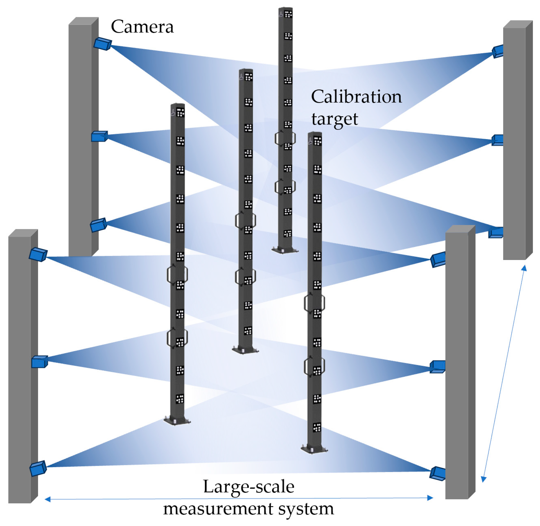
Using large-scale three-coordinate measuring machines or photogrammetry systems for fixed space measurement, a series of industrial cameras distributed throughout the measurement space are used to construct a fixed measurement field, as shown in Figure 1. By calibrating the internal and external parameters between multiple cameras and utilizing the measurement adjustment model, the system calibration of the measurement is completed. Then the spatial point measurement can be carried out with the measurement light pen.

However, there is a lack of evaluation methods for the accuracy of spatial point measurement. Due to the complexity of the industrial manufacturing site, when performing accuracy detection of key point positions of products, it is still necessary to evaluate the accuracy of point position measurement in the measurement field. As a commonly used length standard, the calibration rod evaluates the spatial point position measurement error through the length measurement error. By establishing the mapping relationship between the length measurement error and the point position error of the calibration rod, the accuracy of point position measurements in the measurement field is calibrated.

2.1. Mapping Model of Spatial Point Measurement Error and Length Measurement Error

Within the range of the large-scale fixed high-precision measurement system, all measurement spaces are included. Suppose the true value of the coordinates of any point in this space is (x_n, y_n, z_n), and the measured value of the point coordinates under the measurement system is (x_n + ∆x_n, y_n + ∆y_n, z_n + ∆z_n). The deviation of the point is δ_n, and the limit measurement positioning deviation of the spatial point is δ_p.

At this time, P₁ and P₂ are two points measured in the measurement system. The true values of P₁ and P₂ are (x₁, y₁, z₁) and (x₂, y₂, z₂) respectively, and their measured values are (x₁ + ∆x₁, y₁ + ∆y₁, z₁ + ∆z₁) and (x₂ + ∆x₂, y₂ + ∆y₂, z₂ + ∆z₂).

The true value of the distance between P₁ and P₂ is L, which can be expressed according to the spatial distance equation:

$$L=\sqrt{{(x_2-x_1)}^2+{(y_2-y_1)}^2+{(z_2-z_1)}^2}=\sqrt{{\left(\Delta x\right)}^2+{\left(\Delta y\right)}^2+{\left(\Delta z\right)}^2}$$

(1)

where ∆x = x₂ − x₁, ∆y = y₂ − y₁, ∆z = z₂ − z₁. Since the distance between P₁ and P₂ is fixed, one point can be regarded as the center of the sphere, and the other point can be regarded as a point on the spherical surface with a radius of L. The difference between the true values of the two points can also be converted to spherical coordinates:

$$\left\{\begin{array}{c}\Delta x=L\times \cos {\alpha }_0\times \cos {\beta }_0\\ \Delta y=L\times \cos {\alpha }_0\times \sin {\beta }_0\\ \Delta z=L\times \sin {\alpha }_0\end{array}\right.$$

(2)

where α₀ ∈ [−π/2,π/2], β₀ ∈ [−π,π]. Figure 2 illustrates the randomly distributed measurement error of the point position. The true length of the calibration rod is denoted as L. The radius of the measurement error distribution interval for spatial point P₁ is δ₁, while for spatial point P₂, it is δ₂.

The distance between P₁ and P₂ is measured as L + ∆L, where ∆L represents the variation in length L, indicating the length measurement error in the distance between P₁ and P₂.

$$L+\Delta L=\sqrt{{\left(x_2+\Delta x_2-x_1-\Delta x_1\right)}^2+{\left(y_2+\Delta y_2-y_1-\Delta y_1\right)}^2+{\left(z_2+\Delta z_2-z_1-\Delta z_1\right)}^2}$$

(3)

The point deviation is converted to spherical coordinate representation:

$$\left\{\begin{array}{c}\Delta x_n={\delta }_n\times \cos {\alpha }_n\times \cos {\beta }_n\\ \Delta y_n={\delta }_n\times \cos {\alpha }_n\times \sin {\beta }_n\\ \Delta z_n={\delta }_n\times \sin {\alpha }_n\end{array}\right.$$

(4)

where α_n ∈ [−π/2,π/2], β_n ∈ [−π,π].

By substituting Equations (2) and (4) into Equation (3), we can obtain:

$$\begin{array}{c}\Delta L+\Delta L^2/2L=M\\ M=\cos {\alpha }_0\cos {\beta }_0({\delta }_2\cos {\alpha }_2\cos {\beta }_2-{\delta }_1\cos {\alpha }_1\cos {\beta }_1)\\ +\cos {\alpha }_0\sin {\beta }_0({\delta }_2\cos {\alpha }_2\sin {\beta }_2-{\delta }_1\cos {\alpha }_1\sin {\beta }_1)\\ +\sin {\alpha }_0({\delta }_2\sin {\alpha }_2-{\delta }_1\sin {\alpha }_1)\end{array}$$

(5)

∆L can be expressed as:

$$\Delta L=\sqrt{L^2+2L{M}^2}-L$$

(6)

It can be proven that the maximum value of M can be obtained when α₀ is in the range of [−π/2,0] and β₀ is in the range of [0, π/2], in which case both δ₁ and δ₂ need to be equal to δ_p.

$$\begin{array}{c}M\le \left|G{\delta }_p\right|\\ G=\cos {\alpha }_0\cos {\beta }_0(\cos {\alpha }_2\cos {\beta }_2-\cos {\alpha }_1\cos {\beta }_1)\\ +\cos {\alpha }_0\sin {\beta }_0(\cos {\alpha }_2\sin {\beta }_2-\cos {\alpha }_1\sin {\beta }_1)\\ +\sin {\alpha }_0(\sin {\alpha }_2-\sin {\alpha }_1)\end{array}$$

(7)

By substituting Equation (7) into Equation (6), the following can be obtained:

$$\Delta L/G+\Delta L^2/2GL\le \left|{\delta }_p\right|$$

(8)

When ∆L approaches the limiting deviation of the measurement δ_L, the equality holds in this case:

$$\left|{\delta }_p\right|={\delta }_L/G+{\delta }_L^2/2GL$$

(9)

2.2. Mapping Model of the Limit Deviation and the Maximum Measurement Deviation

When measuring the length of the standard rod in the measurement system, we encounter a length error at the micron level. Therefore, we do not consider the measurement error caused by the length of the standard rod.

We placed a standard rod with a length of L in multiple positions in the measurement system, measured it n times in different orientations, and covered as many common measurement positions as possible, ensuring that the position was as random as possible. We recorded the length measurement value L_n given by the measurement system each time. It was difficult to obtain the limit deviation in a finite number of measurements. Based on the generalized extreme value distribution and the cumulative probability quantile, the relationship between the maximum measurement deviation ∆L_max and the limit length deviation δ_L was established.

As ∆L_max represents the extreme value distribution of multiple measurements, it can be determined that it follows the generalized extreme value distribution. When conducting n measurements, it is necessary to calculate the probability P of obtaining a maximum value exceeding a specific threshold, as well as the corresponding cumulative probability quantile F of ∆L.

$$\mathrm{F}=\frac{\sqrt[n]{1+\mathrm{P}}}{2}+0.5$$

(10)

The independent variable Fα corresponding to the quantile F is the factor for which the maximum value δ_L is obtained with probability P.

The discrete results of the cumulative probability distribution function of ∆L distributed in the interval (−1, 1) can be provided. Since it is symmetric about the y-axis, only the table for Fα > 0 is listed in

Table 1. F-distribution quantile comparison table.

Fα	F	Fα	F	Fα	F
0.00	0.500	0.34	0.773	0.68	0.931
0.02	0.523	0.36	0.785	0.7	0.938
0.04	0.543	0.38	0.796	0.72	0.944
0.06	0.563	0.4	0.808	0.74	0.950
0.08	0.582	0.42	0.818	0.76	0.956
0.1	0.600	0.44	0.829	0.78	0.962
0.12	0.617	0.46	0.839	0.8	0.967
0.14	0.634	0.48	0.849	0.82	0.971
0.16	0.651	0.5	0.858	0.84	0.976
0.18	0.666	0.52	0.868	0.86	0.980
0.2	0.681	0.54	0.876	0.88	0.984
0.22	0.696	0.56	0.885	0.9	0.988
0.24	0.710	0.58	0.893	0.92	0.991
0.26	0.723	0.6	0.901	0.94	0.994
0.28	0.736	0.62	0.909	0.96	0.996
0.3	0.749	0.64	0.917	0.98	0.999
0.32	0.761	0.66	0.924	1	1.000

:

When the measurement is performed n times, the maximum deviation of the length value is greater than Fα with probability P. Let (1 − P) be sufficiently small (generally less than 1%). According to Equation (10), the corresponding quantile F of the cumulative probability distribution of ∆L_max is calculated. After obtaining F, the corresponding Fα can be queried in Table 1.

When the number of measurements is n times, the probability that ∆L_max is greater than Fα is P. It can be considered that when the measurement is performed n times:

$$\Delta L_{\max }\ge {\delta }_L\times F\alpha$$

(11)

2.3. Calculate the Spatial Positioning Accuracy Based on the Maximum Measurement Deviation

Statistically, the maximum measurement deviation ∆L_max is obtained by subtracting the standard length L from each length L_n in the measurement of the standard rod n times.

Substituting Equation (11) into Equation (9), we can obtain:

$${\delta }_p\le \frac{\Delta L_{\max }/F\alpha }{G}+\frac{{\left(\Delta L_{\max }/F\alpha \right)}^2}{2GL}$$

(12)

When δ_L approaches the maximum deviation of the measured value, G = 2:

$${\delta }_p\le \frac{\Delta L_{\max }/F\alpha }{2}+\frac{{\left(\Delta L_{\max }/F\alpha \right)}^2}{4L}$$

(13)

δ_p is the spatial point measurement accuracy of the measurement system.

Based on the derivation process mentioned above, we achieved point measurement accuracy evaluation for a large-scale fixed measurement field. As shown in Figure 3, we have plotted the flowchart of this algorithm to demonstrate the simplicity of the proposed method.

3. Experiment

A large-scale fixed measurement field utilizing photogrammetry technology was applied to the experimental verification platform to validate the effectiveness of the algorithm and model. The measurement station comprised a 20-camera array, with the spatial positions of the cameras needing to cover the envelope space of the target object. Each camera had an imaging resolution of 5120 × 5120 pixels and a 25-mm imaging lens. This ensured that at least two cameras could capture each identification point distributed in the measurement area. After visibility analysis, the spatial positions of the cameras could be fixed to form a large-scale fixed measurement field.

According to the binocular vision measurement mathematical model, in order to calculate the coordinate values of spatial points, it is necessary to calibrate the internal and external parameters of the camera array contained in a large-scale fixed measurement field. In this system, the internal parameters of the cameras are calibrated individually before the construction of the measurement field, while the external parameters of each camera need to be calibrated on site due to differences in installation position or arrangement. To improve the calibration efficiency, as shown in Figure 4, the calibration target was used to calibrate the external parameters of the cameras in the measurement field.

Multiple calibration images were captured using a known-length reference calibration scale that moved freely within the shared visual field of multiple cameras. Image processing was employed to acquire multiple sets of image point coordinates. By leveraging the geometric relationship between views, relative orientation is achieved, and by utilizing the known length, absolute orientation is determined. Through iteration, the precise structural parameters of the camera group are obtained. The calibration of the large-scale fixed measurement field is thus completed.

After the calibration is completed, the calibration accuracy analysis focuses solely on the measurement error of the camera system. However, it is not possible to quantify the measurement accuracy of the measurement rod. In this paper, a calibration rod of length 2286.291 mm is used for calibration. Equation (14) is used to establish the relationship of spatial point measurement accuracy with the calibration rod.

$$\left|{\delta }_p\right|={\delta }_L/2+{\delta }_L^2/9145.164$$

(14)

The calibration rod was randomly placed in different positions in the measurement system, and 50 measurements were taken to calculate the difference between each measurement length and the actual length of the calibration rod. The actual data are as follows.

The relationship between the theoretical maximum measurement error and the maximum measurement error of the finite measurements was calculated. According to

Table 2. Length measurement error data for the calibration rod in 50 groups.

Position	∆L (mm)	Position	∆L (mm)	Position	∆L (mm)	Position	∆L (mm)	Position	∆L (mm)
A1	0.003	A11	−0.005	A21	0.157	A31	0.04	A41	0.106
A2	0.022	A12	−0.079	A22	0.035	A32	−0.123	A42	0.118
A3	0.079	A13	0.043	A23	0.112	A33	−0.02	A43	0.001
A4	−0.01	A14	0.113	A24	0.028	A34	0.013	A44	0.044
A5	0.106	A15	−0.055	A25	0.169	A35	−0.001	A45	0.138
A6	0.011	A16	−0.082	A26	0.125	A36	−0.016	A46	0.043
A7	0.125	A17	0.022	A27	0.063	A37	0.016	A47	0.083
A8	0.052	A18	0.026	A28	0.037	A38	−0.019	A48	0.101
A9	−0.005	A19	0.16	A29	0.037	A39	0.023	A49	0.071
A10	−0.023	A20	0.099	A30	−0.078	A40	0.161	A50	0.006

, the maximum measurement error was ∆L_max = 0.169, which indicates the highest possible deviation in the recorded measurements. When n = 50 and P = 99%, substituting the values into Equation (10), F = 0.9560. By looking up the value in the F-distribution quantile comparison table, the corresponding Fα was found to be 0.7603. Then, δ_L ≤ 0.169/0.7603 = 0.2223. Based on the maximum measurement error δ_L, the spatial point accuracy was calculated as δ_p ≤ 0.1111 by substituting the value into Equation (14).

A value of δ_p = 0.1111 was substituted into the Monte Carlo simulation, and 100,000 simulations were performed, with each simulation including 50 measurements. The distribution of the maximum measurement error in 100,000 simulations is shown in Figure 5a by applying Equation (10) of the technical scheme for simulation. It can be seen that the actual maximum error of 0.169 is within this distribution and corresponds to the 0.01 quantile value. The limit measurement error was 0.22, which is highly consistent with the maximum measurement error of 0.2223 obtained previously.

In the 100,000 simulations, the distribution of the spatial point measurement accuracy is shown in Figure 5b. It can be seen that the upper limit of the spatial point measurement accuracy obtained through the Monte Carlo simulation is 0.1462, which is highly consistent with the spatial point measurement accuracy of 0.1111/0.7603 = 0.146 obtained from the finite sampling.

4. Discussion and Conclusions

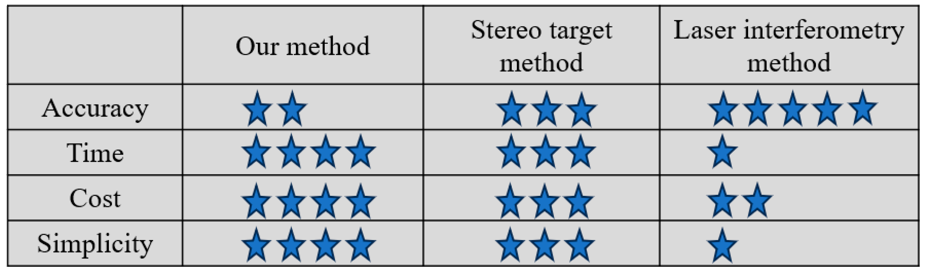
The precision of point positioning in the manufacturing of large-scale components is a fundamental factor that influences both the structural integrity and the assembly efficiency of the overall machinery. To evaluate the manufacturing and assembly quality of large-scale equipment with greater accuracy, efficiency, and scope, assessing the positioning accuracy of these components is crucial. This study introduces a fast evaluation method for positioning measurement accuracy with a stationary measurement setup. This method significantly streamlines the conventional calibration process; using only a calibration rod, the positioning measurement accuracy of an extensive, stationary measurement system can be calibrated, circumventing the need for intricate tools such as laser interferometers and precision displacement platforms. We compared our method with other techniques, such as the laser interferometer calibration method [29] and the stereo target calibration method [30]. As shown in Figure 6, when using the laser interferometry method for large-scale measurement field calibration, it is often necessary to use a translation slide for measurement. This evaluation method can achieve micron-level measurement accuracy. However, setting up a high-linearity translation device such as a slide track is time-consuming. The stereo target method requires the distribution of stereo calibration points in space to complete the accuracy evaluation. In applications prioritizing efficiency and simplicity, our method can be preferentially used for rapid accuracy verification. It should be noted that if the verification results indicate a significant measurement deviation, re-calibration using a stereo target method is still necessary.

The proposed method has the potential to achieve a calibration precision within 0.1 mm for a measurement scope of up to 20 m, enabling rapid and precise calibration of expansive measurement areas. The proposed model elucidates the relationship between spatial point measurement accuracy and length measurement error. To further analyze the accuracy model of this method, error sources in the process were analyzed. The error sources affecting the final measurement accuracy evaluation include the following: (1) spatial layout of the calibration rod in the measurement system (distances between the camera and markers, attitudes between the camera and markers, marker sizes, etc.); (2) reference point extraction calculation method (image processing algorithm); (3) environmental factors (measurement environment vibration, light pollution, etc.) and system calibration error; (4) manufacturing error of the calibration rod. Due to the manufacturing error of the calibration rod being much smaller than the measured scale, the impact is negligible. The most significant influence is the size of the marker on the image, which is a result of the combined effects of the measurement system, the relative positions of the marker and camera, and the camera calibration parameters. The optimal size of the marker on the image is 5–15 pixels.

In conclusion, the calibration technique presented in this research represents a practical and efficient solution for verifying the accuracy of positioning measurements on large-scale equipment. This streamlined process not only enhances our insights into manufacturing errors but also supports the structural integrity and assembly efficiency of machinery. Future improvements can be made in the following directions:

• The error distribution model of the fixed measurement field can be studied to improve the limit mapping model of the measurement length in the algorithm, thereby enhancing the spatial point measurement accuracy in the fixed measurement field.
• An accuracy evaluation method based on a three-dimensional digital model of the workpiece can be developed to avoid measurement errors caused by poor spatial position distribution in the measurement system.