
Optimization of Integrated Energy Systems Based on Two-Step Decoupling Method


 , and
, and
Abstract
1. Introduction
2. Materials and Methods
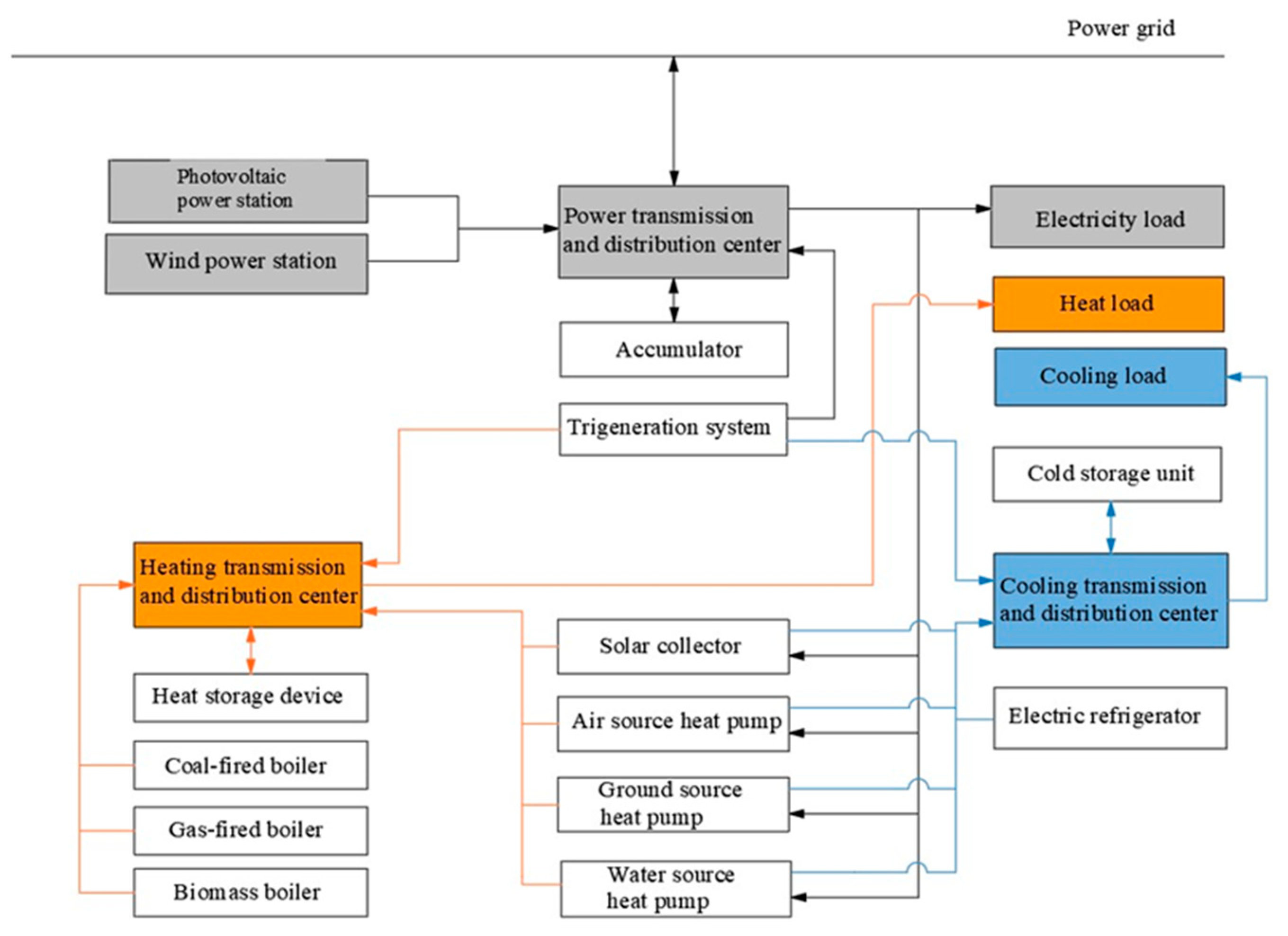
2.1. The Decoupling of a Generalized Structure of an IES
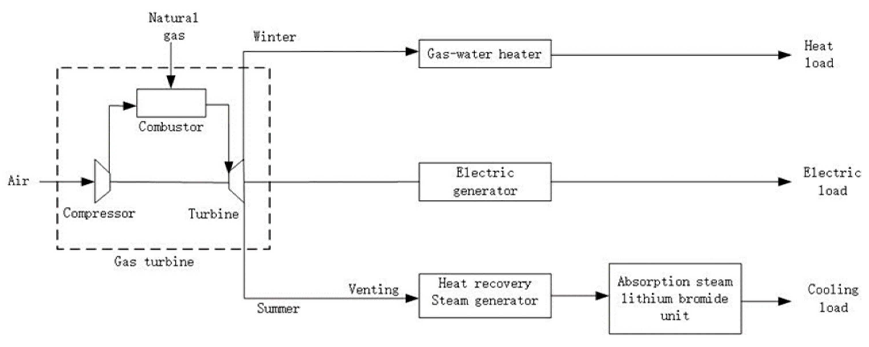
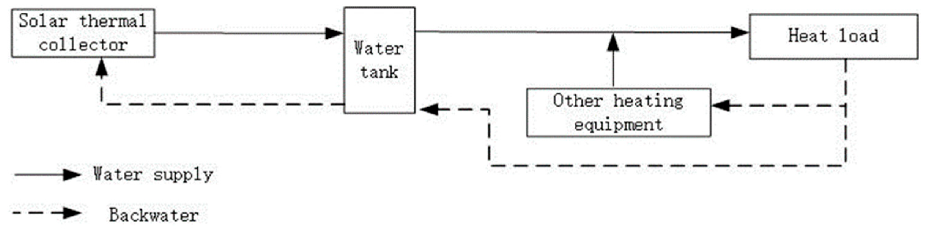
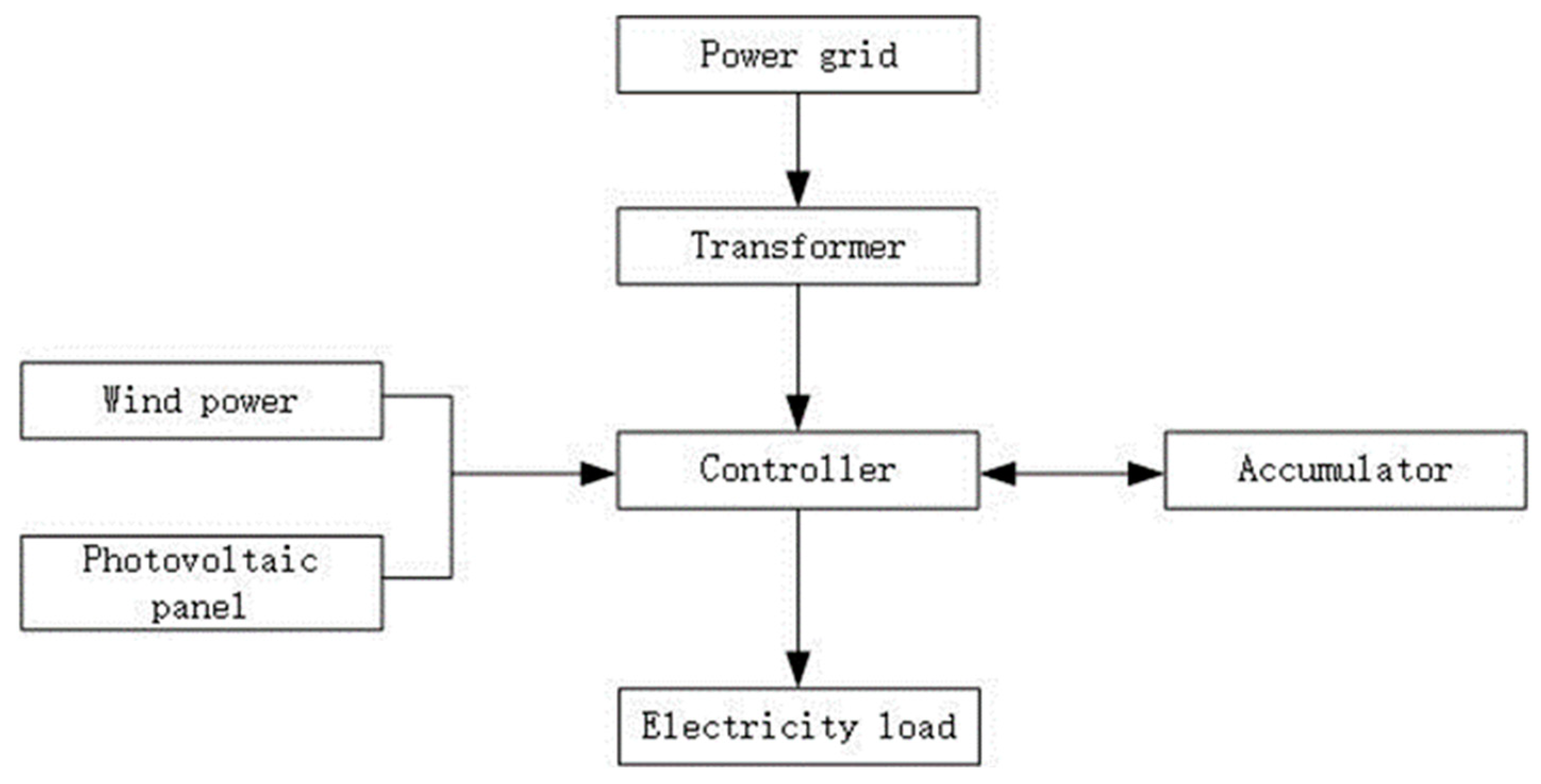
2.2. Mathematical Models of the Subsystems
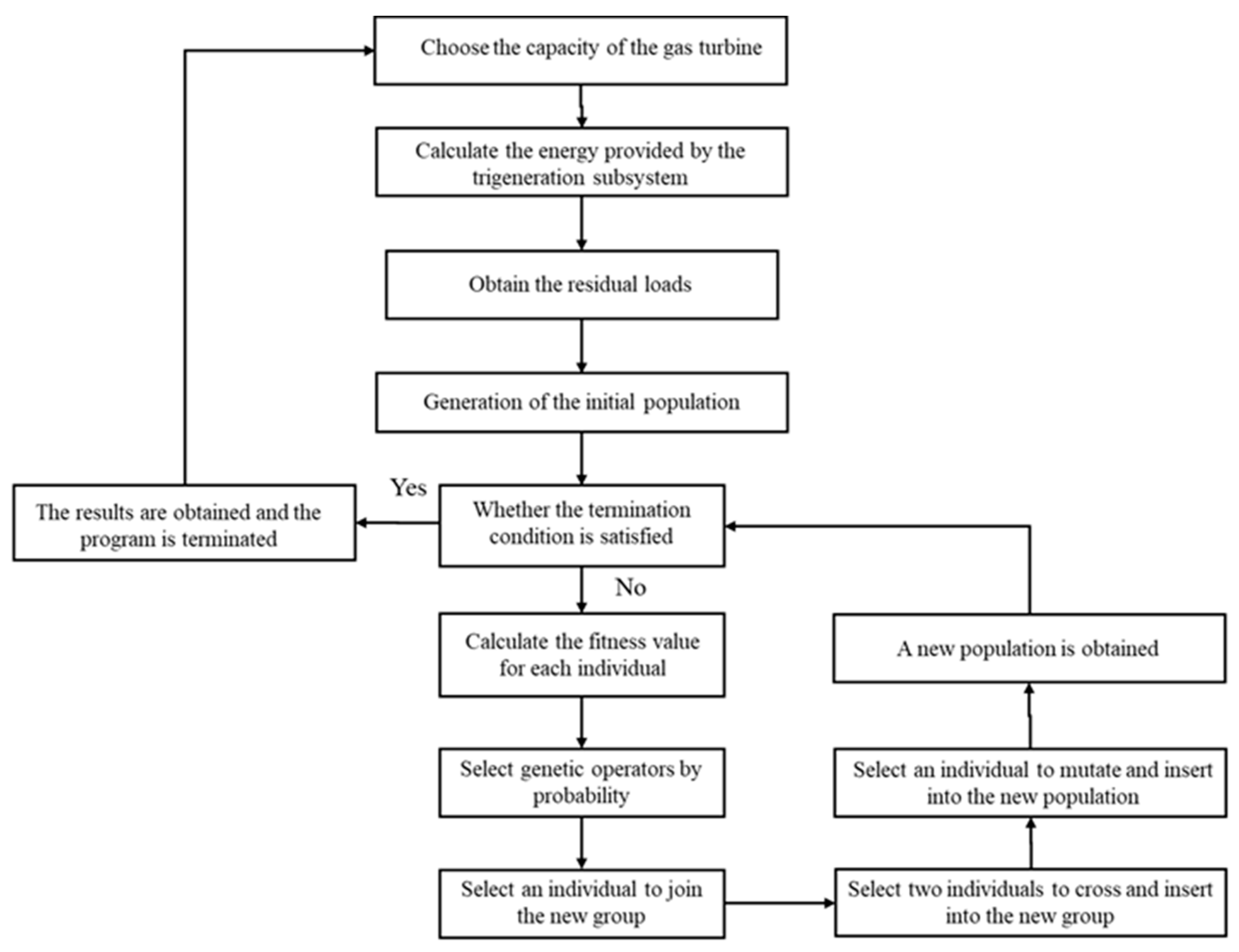
2.3. A Two-Layer Optimization Method
3. Results and Discussion
4. Conclusions
Author Contributions
Funding
Data Availability Statement
Conflicts of Interest
References
- Song, C.; Jing, W.; Zeng, P.; Rosenberg, C. An analysis on the energy consumption of circulating pumps of residential swimming pools for peak load management. Appl. Energy 2017, 195, 1–12. [Google Scholar] [CrossRef]
- Kanchev, H.; Lu, D.; Colas, F.; Lazarov, V.; Francois, B. Energy management and operational planning of a microgrid with a PV-based active generator for smart grid applications. IEEE Trans. Ind. Electron. 2011, 58, 4583–4592. [Google Scholar] [CrossRef]
- Zhang, S.; Wang, T.; Gao, Z.; Zhang, Y. Wettability controlling effects on the fluid occurrence and flow in shale gas reservoirs: Present problems and new sights. Capillarity 2023, 9, 25–31. [Google Scholar] [CrossRef]
- Tu, Y.; Zhang, Y.; Dong, Y.; Ma, Y. Adsorption and desorption characteristics of coal seam gas under infrared radiation. Capillarity 2023, 8, 53–64. [Google Scholar] [CrossRef]
- Yang, Y.; Li, Z.; Mandapaka, P.V.; Lo, E.Y. Risk-averse restoration of coupled power and water systems with small pumped-hydro storage and stochastic rooftop renewables. Appl. Energy 2023, 339, 120953. [Google Scholar] [CrossRef]
- Farrokhifar, M.; Nie, Y.; Pozo, D. Energy systems planning: A survey on models for integrated power and natural gas networks coordination. Appl. Energy 2020, 262, 114567. [Google Scholar] [CrossRef]
- Chen, H.; Wang, X.; Li, Z.; Chen, W.; Cai, Y. Distributed sensing and cooperative estimation/detection of ubiquitous power internet of things. Prot. Control Mod. Power Syst. 2019, 4, 13. [Google Scholar] [CrossRef]
- Liserre, M.; Sauter, T.; Hung, J.Y. Future energy systems: Integrating renewable energy sources into the smart power grid through industrial electronics. IEEE Ind. Electron. Mag. 2010, 4, 18–37. [Google Scholar] [CrossRef]
- Huang, H.; Li, Z.; Sampath, L.P.M.I.; Yang, J.; Nguyen, H.D.; Gooi, H.B.; Liang, R.; Gong, D. Blockchain-Enabled Carbon and Energy Trading for Network-Constrained Coal Mines with Uncertainties. IEEE Trans. Sustain. Energy 2023, 14, 1634–1647. [Google Scholar] [CrossRef]
- Khalilpour, K.R.; Vassallo, A. A generic framework for distributed multi-generation and multi-storage energy systems. Energy 2016, 114, 798–813. [Google Scholar] [CrossRef]
- Zhou, Y.; Wei, Z.; Sun, G.; Cheung, K.W.; Zang, H.; Chen, S. A robust optimization approach for integrated community energy system in energy and ancillary service markets. Energy 2018, 148, 1–15. [Google Scholar] [CrossRef]
- Wang, Y.; Huang, Y.; Wang, Y.; Yu, H.; Li, R.; Song, S. Energy Management for Smart Multi-Energy Complementary Micro-Grid in the Presence of Demand Response. Energies 2018, 11, 974. [Google Scholar] [CrossRef]
- Li, Z.; Xu, Y.; Wang, P.; Xiao, G. Coordinated preparation and recovery of a post-disaster Multi-energy distribution system considering thermal inertia and diverse uncertainties. Appl. Energy 2023, 336, 120736. [Google Scholar] [CrossRef]
- Riaz, M.; Ahmad, S.; Naeem, M. Joint energy management and trading among renewable integrated microgrids for combined cooling, heating, and power systems. J. Build. Eng. 2023, 75, 106921. [Google Scholar] [CrossRef]
- Li, Z.; Xu, Y.; Wang, P.; Xiao, G. Restoration of Multi Energy Distribution Systems With Joint District Network Recon Figuration by a Distributed Stochastic Programming Approach. IEEE Trans. Smart Grid 2023, 15, 2667–2680. [Google Scholar] [CrossRef]
- Quelhas, A.; Gil, E.; McCalley, J.D.; Ryan, S.M. A multiperiod generalized network flow model of the U.S. integrated energy system: Part I—Model description. IEEE Trans. Power Syst. 2007, 22, 829–836. [Google Scholar] [CrossRef]
- Zhu, M.; Xu, C.; Dong, S.; Tang, K.; Gu, C. An integrated multi-energy flow calculation method for electricity-gas-thermal integrated energy systems. Prot. Control Mod. Power Syst. 2021, 6, 5. [Google Scholar] [CrossRef]
- Li, J.; Li, D.; Zheng, Y.; Yao, Y.; Tang, Y. Unified modeling of regionally integrated energy system and application to optimization. Int. J. Electr. Power Energy Syst. 2022, 134, 107377. [Google Scholar] [CrossRef]
- Martinez-Mares, A.; Fuerte-Esquivel, C.R. A unified gas and power flow analysis in natural gas and electricity coupled networks. IEEE Trans. Power Syst. 2012, 27, 2156–2166. [Google Scholar] [CrossRef]
- He, C.; Dai, C.; Wu, L.; Liu, T. Robust network hardening strategy for enhancing resilience of integrated electricity and natural gas distribution systems against natural disasters. IEEE Trans. Power Syst. 2018, 33, 5787–5798. [Google Scholar] [CrossRef]
- Shabanpour-Haghighi, A.; Seifi, A.R. Simultaneous integrated optimal energy flow of electricity, gas, and heat. Energy Convers. Manag. 2015, 101, 579–591. [Google Scholar] [CrossRef]
- Zhang, D.; Evangelisti, S.; Lettieri, P.; Papageorgiou, L.G. Optimal design of CHP-based microgrids: Multiobjective optimisation and life cycle assessment. Energy 2015, 85, 181–193. [Google Scholar] [CrossRef]
- Qin, C.; Wang, L.; Han, Z.; Zhao, J.; Liu, Q. Weighted directed graph based matrix modeling of integrated energy systems. Energy 2021, 214, 118886. [Google Scholar] [CrossRef]
- Sun, Q.; Chen, Y. Multi-Energy Flow Calculation Method for We-Energy Based Energy Internet. In Proceedings of the 1st IEEE International Conference on Energy Internet, ICEI 2017, Beijing, China, 17–21 April 2017; pp. 30–35. [Google Scholar] [CrossRef]
- Qin, X.; Sun, H.; Shen, X.; Guo, Y.; Guo, Q.; Xia, T. A generalized quasi-dynamic model for electric-heat coupling integrated energy system with distributed energy resources. Appl. Energy 2019, 251, 113270. [Google Scholar] [CrossRef]
- Mohammadi, M.; Noorollahi, Y.; Mohammadi-Ivatloo, B.; Yousefi, H. Energy hub: From a model to a concept—A review. Renew. Sustain. Energy Rev. 2017, 80, 1512–1527. [Google Scholar] [CrossRef]
- Beigvand, S.D.; Abdi, H.; La Scala, M. A general model for energy hub economic dispatch. Appl. Energy 2017, 190, 1090–1111. [Google Scholar] [CrossRef]
- Hao, R.; Ai, Q.; Jiang, Z. Bilayer game strategy of regional integrated energy system under multi-agent incomplete information. J. Eng. 2019, 2019, 1285–1291. [Google Scholar] [CrossRef]
- Wang, Y.; Huang, Y.; Wang, Y.; Zeng, M.; Yu, H.; Li, F.; Zhang, F. Optimal scheduling of the RIES considering time-based demand response programs with energy price. Energy 2018, 164, 773–793. [Google Scholar] [CrossRef]
- Gao, Y.; Ai, Q. Hierarchical Coordination Control for Interconnected Operation of Electric-thermal-gas Integrated Energy System with Micro-energy Internet Clusters. IEEE J. Emerg. Sel. Top. Power Electron. 2018. [Google Scholar] [CrossRef]
- Fu, X.; Zhang, X. Failure probability estimation of gas supply using the central moment method in an integrated energy system. Appl. Energy 2018, 219, 1–10. [Google Scholar] [CrossRef]
- Ma, W.; Fang, S.; Liu, G. Hybrid optimization method and seasonal operation strategy for distributed energy system integrating CCHP, photovoltaic and ground source heat pump. Energy 2017, 141, 1439–14555. [Google Scholar] [CrossRef]
- Chen, Y.; Wei, W.; Liu, F.; Wu, Q.; Mei, S. Analyzing and validating the economic efficiency of managing a cluster of energy hubs in multi-carrier energy systems. Appl. Energy 2018, 230, 403–416. [Google Scholar] [CrossRef]
- Geidl, M.; Koeppel, G.; Favre-Perrod, P.; Klöckl, B.; Andersson, G.; Fröhlich, K. The Energy Hub—A Powerful Concept for Future Energy Systems. In Proceedings of the Third Annual Carnegie Mellon Conference on the Electricity Industry, Pittsburgh, PA, USA, 13–14 March 2007. [Google Scholar]
- Evins, R.; Pointer, P.; Vaidyanathan, R.; Burgess, S. A case study exploring regulated energy use in domestic buildings using design-of-experiments and multi-objective optimization. Build. Environ. 2012, 54, 126–136. [Google Scholar] [CrossRef]
- Nguyen, A.-T.; Reiter, S.; Rigo, P. A review on simulation-based optimization methods applied to building performance analysis. Appl. Energy 2014, 113, 1043–1058. [Google Scholar] [CrossRef]
- Machairas, V.; Tsangrassoulis, A.; Axarli, K. Algorithms for optimization of building design: A review. Renew. Sustain. Energy Rev. 2014, 31, 101–112. [Google Scholar] [CrossRef]
- Evins, R. A review of computational optimisation methods applied to sustainable building design. Renew. Sustain. Energy Rev. 2013, 22, 230–245. [Google Scholar] [CrossRef]
- Ferrara, M.; Fabrizio, E.; Virgone, J.; Filippi, M. A simulation-based optimization method for cost-optimal analysis of nearly Zero Energy Buildings. Energy Build. 2014, 84, 442–457. [Google Scholar] [CrossRef]
- Niu, D.; Wang, Y.; Wu, D.D. Power load forecasting using support vector machine and ant colony optimization. Expert Syst. Appl. 2010, 37, 2531–2539. [Google Scholar] [CrossRef]
- Wu, Q.; Ren, H.; Gao, W.; Ren, J. Modeling and optimization of distributed energy supply network with power and hot water interchanges. Appl. Therm. Eng. 2016, 94, 635–643. [Google Scholar] [CrossRef]
- Lorestani, A.; Ardehali, M. Optimal integration of renewable energy sources for autonomous tri-generation combined cooling, heating and power system based on evolutionary particle swarm optimization algorithm. Energy 2018, 145, 839–855. [Google Scholar] [CrossRef]
- Li, Y.; Liang, W.; Tan, R. Optimal design of installation capacity and operation strategy for distributed energy system. Appl. Therm. Eng. 2017, 125, 756–766. [Google Scholar] [CrossRef]
- Urbanucci, L.; Testi, D. Optimal integrated sizing and operation of a CHP system with Monte Carlo risk analysis for long-term uncertainty in energy demands. Energy Convers. Manag. 2018, 157, 307–316. [Google Scholar] [CrossRef]
- Guo, L.; Liu, W.J.; Cai, J.J.; Hong, B.W.; Wang, C.S. A two-stage optimal planning and design method for combined cooling, heat and power microgrid system. Energy Convers. Manag. 2013, 74, 433–445. [Google Scholar] [CrossRef]
- Li, B.; Roche, R.; Paire, D.; Miraoui, A. Optimal sizing of distributed generation in gas/electricity/heat supply networks. Energy 2018, 151, 675–688. [Google Scholar] [CrossRef]
- Yousefi, H.; Ghodusinejad, M.H.; Noorollahi, Y. GA/AHP-based optimal design of a hybrid CCHP system considering economy, energy and emission. Energy Build. 2017, 138, 309–317. [Google Scholar] [CrossRef]
- Li, M.; Lu, Z.; Kang, Z.; Ban, L.; Cong, H.; Lu, Y. Investigation of an air-cooled double-channel photovoltaic/thermal system with integrated thermal energy storage. J. Build. Eng. 2023, 77, 107539. [Google Scholar] [CrossRef]
- Ameri, M.; Besharati, Z. Optimal design and operation of district heating and cooling networks with CCHP systems in a residential complex. Energy Build. 2016, 110, 135–148. [Google Scholar] [CrossRef]
- Wei, F.; Wu, Q.; Jing, Z.; Chen, J.; Zhou, X. Optimal unit sizing for small-scale integrated energy systems using multi-objective interval optimization and evidential reasoning approach. Energy 2016, 111, 933–946. [Google Scholar] [CrossRef]
- Zhang, L.; Kuang, J.; Sun, B.; Li, F.; Zhang, C. A two-stage operation optimization method of integrated energy systems with demand response and energy storage. Energy 2020, 208, 118423. [Google Scholar] [CrossRef]
- Qin, C.; Yan, Q.; He, G. Integrated energy systems planning with electricity, heat and gas using particle swarm optimization. Energy 2019, 188, 116044. [Google Scholar] [CrossRef]
- Tan, Z.; Yang, S.; Lin, H.; De, G.; Ju, L.; Zhou, F. Multi-scenario operation optimization model for park integrated energy system based on multi-energy demand response. Sustain. Cities Soc. 2020, 53, 101973. [Google Scholar] [CrossRef]
- Wang, Y.; Wang, Y.; Huang, Y.; Yu, H.; Du, R.; Zhang, F.; Zhang, F.; Zhu, J. Optimal Scheduling of the Regional Integrated Energy System Considering Economy and Environment. IEEE Trans. Sustain. Energy 2019, 10, 1939–1949. [Google Scholar] [CrossRef]
- Ma, T.; Wu, J.; Hao, L.; Lee, W.-J.; Yan, H.; Li, D. The optimal structure planning and energy management strategies of smart multi energy systems. Energy 2018, 160, 122–141. [Google Scholar] [CrossRef]
- Fathima, A.H.; Palanisamy, K. Optimization in microgrids with hybrid energy systems—A review. Renew. Sustain. Energy Rev. 2015, 45, 431–446. [Google Scholar] [CrossRef]
- Zhao, N.; Gu, W. Low-carbon planning and optimization of the integrated energy system considering lifetime carbon emissions. J. Build. Eng. 2024, 82, 108178. [Google Scholar] [CrossRef]
- Song, Z.; Hofmann, H.; Li, J.; Han, X.; Ouyang, M. Optimization for a hybrid energy storage system in electric vehicles using dynamic programing approach. Appl. Energy 2015, 139, 151–162. [Google Scholar] [CrossRef]
- Tan, Z.; De, G.; Li, M.; Lin, H.; Yang, S.; Huang, L.; Tan, Q. Combined electricity-heat-cooling-gas load forecasting model for integrated energy system based on multi-task learning and least square support vector machine. J. Clean. Prod. 2020, 248, 119252. [Google Scholar] [CrossRef]
- Shao, Y.; Chen, B.; Xiao, H.; Qin, F.G.F. Discussion on Performance Evaluation Method of Distributed Combined Cooling, Heating, and Power System. J. Therm. Sci. 2019, 28, 1212–1220. [Google Scholar] [CrossRef]
- Zhang, J.; Zhang, S.; Niu, Y. A high proportion of new energy access–combined cooling, heating, and power system planning method. Int. J. Energy Res. 2019, 43, 7942–7955. [Google Scholar] [CrossRef]


| Type of Subsystem | Sequence of Operation for Various Pieces of Equipment |
|---|---|
| Heating subsystem | Solar collector > GSHP > ASHP or biomass boiler > gas-fired boiler > coal-fired boiler |
| Cooling subsystem | GSHP > ASHP > electric chiller |
| Power subsystem | Photovoltaic power or wind power > power grid |
| Sources of Emission | Emission Amount |
|---|---|
| Gas boiler | 0.2556 kg·MWh−1 |
| Absorption chiller | 0.1008 kg·MWh−1 |
| Heat generated by gas turbine | 0.32 kg·MWh−1 |
| Electricity from grid | 2.78 kg·MWh−1 |
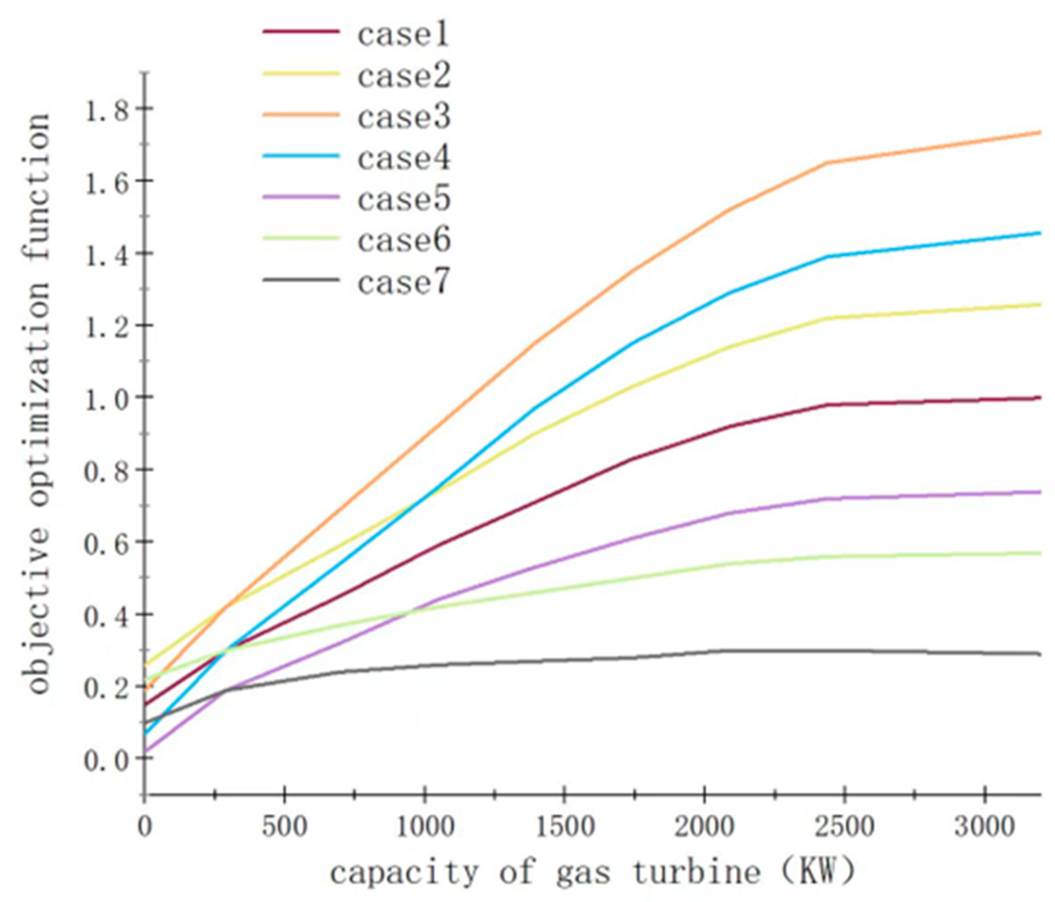
| Case | α | β | γ | Case |
|---|---|---|---|---|
| 1 | 1/3 | 1/3 | 1/3 | 1 |
| 2 | 0 | 2/3 | 1/3 | 2 |
| 3 | 0 | 1/3 | 2/3 | 3 |
| 4 | 1/3 | 0 | 2/3 | 4 |
| 5 | 2/3 | 0 | 1/3 | 5 |
| 6 | 1/3 | 2/3 | 0 | 6 |
| 7 | 2/3 | 1/3 | 0 | 7 |
| Equipment | Price |
|---|---|
| Gas turbine | 4500 CNY/kW |
| Absorption chiller | 455 CNY/kW |
| Gas/water exchanger | 200 CNY/kW |
| HRSG | 120 CNY/kW |
| GSHP | 600 CNY/kW |
| Geothermal well | 7500 CNY/well |
| Gas boiler | 145 CNY/kW |
| Electric chiller | 635 CNY/kW |
| System Configuration | Annual Cost/Ten Thousand Yuan | Primary Energy Consumption/GJ | CO2 Emission/ton | NOX Emission/kg |
|---|---|---|---|---|
| The coupling system | 424 | 11,113 | −1903 | −21,676 |
| The GSHP system | 519 | 41,158 | 3588 | 10,234 |
| The traditional distributed system | 438 | 64,113 | 4893 | 10,106 |
Disclaimer/Publisher’s Note: The statements, opinions and data contained in all publications are solely those of the individual author(s) and contributor(s) and not of MDPI and/or the editor(s). MDPI and/or the editor(s) disclaim responsibility for any injury to people or property resulting from any ideas, methods, instructions or products referred to in the content. |
© 2024 by the authors. Licensee MDPI, Basel, Switzerland. This article is an open access article distributed under the terms and conditions of the Creative Commons Attribution (CC BY) license (https://creativecommons.org/licenses/by/4.0/).
Share and Cite
Zhang, L.; Guo, J.; Yu, X.; Hui, G.; Liu, N.; Ren, D.; Wang, J. Optimization of Integrated Energy Systems Based on Two-Step Decoupling Method. Electronics 2024, 13, 2045. https://doi.org/10.3390/electronics13112045
Zhang L, Guo J, Yu X, Hui G, Liu N, Ren D, Wang J. Optimization of Integrated Energy Systems Based on Two-Step Decoupling Method. Electronics. 2024; 13(11):2045. https://doi.org/10.3390/electronics13112045
Chicago/Turabian StyleZhang, Linyang, Jianxiang Guo, Xinran Yu, Gang Hui, Na Liu, Dongdong Ren, and Jijin Wang. 2024. "Optimization of Integrated Energy Systems Based on Two-Step Decoupling Method" Electronics 13, no. 11: 2045. https://doi.org/10.3390/electronics13112045
APA StyleZhang, L., Guo, J., Yu, X., Hui, G., Liu, N., Ren, D., & Wang, J. (2024). Optimization of Integrated Energy Systems Based on Two-Step Decoupling Method. Electronics, 13(11), 2045. https://doi.org/10.3390/electronics13112045