Abstract
Video summarization aims to analyze the structure and content of videos and extract key segments to construct summarization that can accurately summarize the main content, allowing users to quickly access the core information without browsing the full video. However, existing methods have difficulties in capturing long-term dependencies when dealing with long videos. On the other hand, there is a large amount of noise in graph structures, which may lead to the influence of redundant information and is not conducive to the effective learning of video features. To solve the above problems, we propose a video summarization generation network based on dynamic graph contrastive learning and feature fusion, which mainly consists of three modules: feature extraction, video encoder, and feature fusion. Firstly, we compute the shot features and construct a dynamic graph by using the shot features as nodes of the graph and the similarity between the shot features as the weights of the edges. In the video encoder, we extract the temporal and structural features in the video using stacked L-G Blocks, where the L-G Block consists of a bidirectional long short-term memory network and a graph convolutional network. Then, the shallow-level features are obtained after processing by L-G Blocks. In order to remove the redundant information in the graph, graph contrastive learning is used to obtain the optimized deep-level features. Finally, to fully exploit the feature information of the video, a feature fusion gate using the gating mechanism is designed to fully fuse the shallow-level features with the deep-level features. Extensive experiments are conducted on two benchmark datasets, TVSum and SumMe, and the experimental results show that our proposed method outperforms most of the current state-of-the-art video summarization methods.
1. Introduction
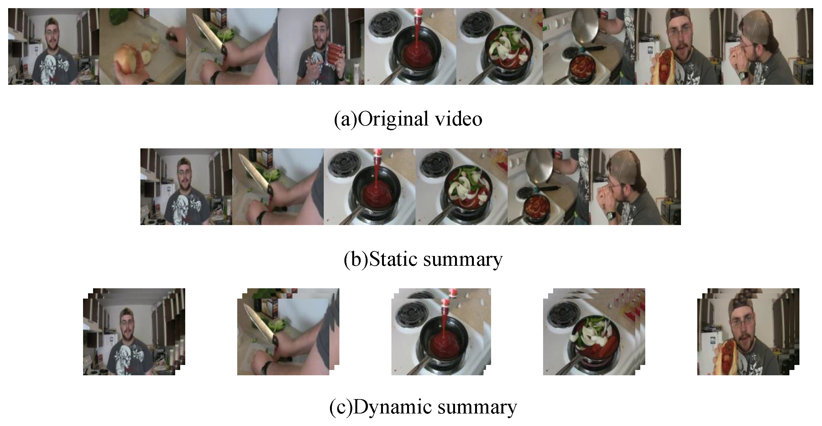
With the rapid growth in video data, efficiently extracting key information from videos has become an important challenge in the field of computer vision. As an important research direction in this field, video summarization has been widely applied in various application scenarios including news, documentaries, surveillance, education, medicine and more. Its main goal is to extract representative frames or shots by analyzing and processing videos and form a short and compact summary video, retaining the key information of the original video as much as possible, so that users can quickly browse and obtain the core information of the video [1,2,3]. According to the type of the generated summaries, video summarization can be generally divided into two types: static video summarization and dynamic video summarization [4]. As shown in Figure 1, static video summarization summarizes the video content through a series of keyframes and generates summaries faster, while dynamic video summarization is composed of several condensed video segments. These segments use shots as their units, integrating image, sound, text and other information and providing richer semantic information. Therefore, we chose dynamic video summarization as the research object.

Figure 1.
Static video summarization and dynamic video summarization.
In long videos, essential information may be distributed throughout the entire sequence, making it difficult for traditional methods to effectively capture these key information. However, deep learning methods, especially those based on recurrent neural networks (RNNs) and long short-term memory networks (LSTMs), have proven effective in overcoming this challenge [5,6]. For instance, Zhao et al. [5] addressed the problem of shot segmentation by designing a sliding Bi-LSTM to detect shot boundaries in videos. They recognized that fixed-length segmentation could disrupt the intrinsic structure of video data and proposed a structure-adaptive video summarization generation method that integrates both video structure and content. However, when processing long video sequences, LSTMs may encounter difficulties in capturing long-term dependencies [7]. Furthermore, since real-world data often exist in non-Euclidean spaces, traditional methods struggle with processing non-Euclidean spatial data. Thus, researchers have introduced graph neural networks (GNNs) [8]. By modeling videos as graphs and employing GNNs, researchers can capture global dependencies and relationships between nodes and edges, effectively utilizing the semantic relationships between video frames. As a result, this approach generated more accurate and comprehensive video summarization [9,10,11]. To address the limitations of traditional sequence models in capturing long-range dependencies, Zhao et al. [9] introduced a reconstructed sequence graph network to capture frame-level temporal dependencies and shot-level global dependencies, thereby improving the preservation of video content and shot-level dependencies. Zhong et al. [10] focused on the challenge of keyframe selection in user-generated videos. Traditional methods often face the problem of high redundancy when processing these videos, so they proposed a video summarization model that combines a graph attention network (GAT) with a bidirectional long short-term memory network (Bi-LSTM). This model first transforms the visual features of images into higher-level features through GAT’s contextual feature transformation mechanism then optimizes the keyframe selection process by combining these high-level visual features with semantic features processed by Bi-LSTM. Zhu et al. [11] suggested a dynamic graph learning approach to capture the spatial representation of video summarization. Unlike traditional methods, they leverage object-level and relationship-level information to build graphs in both space and time then use graph convolutional networks to analyze relationships in spatial and temporal graphs. This approach extracts spatio-temporal video representations for importance score prediction and key shot selection. However, capturing long-term dependencies in video content remains a significant challenge. Additionally, graph structures often contain noise, which can lead to redundant information interfering with video feature learning. Therefore, solving these problems has become a major challenge in the field of video summarization.
In order to solve the above problems, we proposed a video summarization generation network based on dynamic graph contrastive learning and feature fusion, which mainly includes three modules: feature extraction, video encoder and feature fusion. In the feature extraction module, we first segment the video into shots and extract features of each frame, and then select representative frames as shot features. In order to tackle the problem of learning long-term feature dependencies, we introduce graph convolutional networks (GCNs) to encode shot features. Considering the shortcomings of GCNs in temporal context learning, we construct the L-G Block, which realizes the complementary advantages of LSTM in temporal context and GCN in graph structure learning by cross-stacking LSTM and GCN. In order to reduce the influence of redundant information in the graph structure on feature learning, we design a dynamic graph contrastive learning mechanism, which optimizes the graph structure and enhances the learning ability of graph representation by dynamically constructing the video graph structure and graph contrastive learning. Finally, in order to make full use of the semantic information of the video, we design a feature fusion gate to fuse shallow-level and deep-level features and use the fused features to predict the importance score of the shot.
The main contributions of this article are in four areas:
- We designed an L-G Block to achieve the complementary advantages of LSTM in temporal context and GCN in graph structure learning by cross-stacking LSTM and GCN.
- We designed a dynamic graph contrastive learning mechanism to enhance the performance of graph representation learning by dynamically constructing the graph structure and introducing graph contrastive learning.
- We designed a feature fusion gate to fuse the shallow-level and deep-level features of the shot to fully capture the semantic information in the video.
- After sufficient experiments on TVSum and SumMe, the effectiveness of our proposed method is verified, and it is proven that our proposed method is better than most of the current state-of-the-art methods.
The remainder of the article is organized as follows: Section 2 introduces the related work. Section 3 provides a detailed description of the proposed method. Section 4 presents the experimental results and relevant analyses. Finally, conclusions are drawn and future directions are discussed in Section 5.
2. Related Works
2.1. Video Summarization
Currently, video summarization algorithms based on deep learning can be roughly classified into four categories: recurrent neural network-based methods, adversarial-based methods, attention mechanism-based methods, and graph neural network-based methods.
Recurrent neural networks (RNNs), especially long short-term memory networks, have been widely used for processing sequential data. Zhao et al. [5] proposed a hierarchical adaptive RNN structure aimed at effectively learning the underlying structure of videos. This network adopts a two-layer structure, where the first layer is used to segment the video into multiple shots and extract shot features and the second layer utilizes Bi-LSTM to capture the temporal dependencies between shots. Subsequently, Zhao et al. [6] further introduced a tensor-trained hierarchical recursive neural network, which incorporates a tensor training embedding layer to constrain the size of the mapping matrix from features to hidden layers. Adversarial learning-based video summarization methods, such as generative adversarial networks and variational graph autoencoders, generate summaries by reconstructing the original videos. Yuan et al. [12] employed a cyclic consistency adversarial network aimed at maximizing the mutual information between the original and summarized videos. Apostolidis et al. [13] proposed the Adv-Ptr-Der-SUM model within the generative adversarial network framework, consisting of summarizer and discriminator components. Sreeja et al. [14] implemented a video summarization framework based on a multi-stage generative adversarial network for feature extraction and knowledge refinement. The primary stage of this network comprises a generator consisting of convolutional recursive autoencoders and a discriminator for reconstructing videos. Following the adversarial network is the knowledge refinement stage, which employs a simple network to select key frames or segments. Attention-based methods have made significant progress in the field of video summarization due to their alignment with the human thinking habits of selecting key frames. Xiao et al. [15] introduced the query-biased self-attention network, which generates summaries by considering user intent and semantic significance. Zhong et al. [16] constructed an attention-based deep hierarchical LSTM network, utilizing 3DCNN for spatiotemporal feature extraction and designing an attention-based hierarchical LSTM module to capture temporal dependencies between video frames. To comprehensively capture global dependencies between video data, they introduced graph neural networks. This method transforms video data into a graph structure, effectively modeling and extracting global dependencies within the video. Zhong et al. [10] proposed a video summarization model based on graph attention networks and Bi-LSTM to address high redundancy between key frames. This model converts video data into a graph structure, adjusting the weights of graph nodes using graph attention networks within this graph while aggregating information from neighboring nodes to generate higher-level visual features. Zhao et al. [9] introduced a reconstruction sequence graph network, hierarchically encoding frames and shots into sequences and graphs, where frame-level dependencies are encoded by long short-term memory networks and shot-level dependencies are captured by graph convolutional networks. Finally, local and global dependencies between shots are utilized for summarization. To capture spatiotemporal dependencies in videos, Zhu et al. [11] constructed a spatial graph based on detected target objects, utilizing the aggregated representation of this spatial graph to construct a temporal graph. Subsequently, they employed graph convolutional networks for relational reasoning on the spatial and temporal graphs and extracted spatiotemporal representations. Additionally, they designed a self-attention edge pooling module to eliminate redundancy in relationships between nodes.
2.2. Graph Neural Networks
Graph neural networks (GNNs) are a type of neural network specifically designed for processing graph-structured data, enabling the transformation of videos into graph structures to handle this non-Euclidean spatial data [8]. However, due to the diversity and complexity of video data, GNNs may face the risk of overfitting when dealing with graph-structured data. Graph convolutional neural networks, as a branch of GNNs, employ a low-dimensional vector to represent the high-dimensional information of nodes in a graph, enabling the capture of global information and better representation of node features. Therefore, to address the challenges of GNNs and better explore the hidden structural relationships in videos, Kipf et al. [17] utilized graph convolutional neural networks to learn the topological structure of graphs, expanding linearly with the number of graph edges, and learning representations of hidden layers to simultaneously encode local graph structures and node features. Wu et al. [3] applied graph convolutional neural networks to multi-video summarization tasks, interpreting graph convolution as an integral transformation of embedding functions under probability measures, using simplified convolution operations to aggregate neighborhood information, and saving computational costs while further efficiently extracting features. Subsequently, Wu et al. [18] proposed dynamic graph convolutional networks, treating multi-video summarization tasks as graph analysis tasks, utilizing graph convolutional networks to learn the evolving dependencies of graph nodes and outputting prediction labels for each shot based on the learned dependencies, thereby measuring the importance and relevance of each video shot within its own video and the entire video collection.
In summary, GNNs can capture dependencies and interactions between nodes, while graph convolutional networks, as a variant of GNNs, can aggregate neighborhood information to effectively extract features. Moreover, by stacking multiple layers of graph convolutional layers, GCNs can learn deep-level feature representations of nodes, enabling the model to capture more complex and abstract graph structural features.
2.3. Graph Contrastive Learning
Contrastive learning methods have gained popularity in self-supervised learning, as they can learn effective data representations by contrasting positive and negative samples. P. Velickovic et al. [19] proposed the DGI algorithm as a general method for unsupervised learning of node representations in graph-structured data. DGI utilizes graph convolutional structures to maximize local mutual information between graph patches and graph summaries. However, DGI cannot guarantee that graph embeddings fully extract useful information. Inspired by the success of DGI, Zhu et al. [20] introduced a new unsupervised graph contrastive learning framework, GRACE, which maximizes the consistency of node embeddings by masking node features and randomly deleting edges and using contrastive loss. Li et al. [21] proposed the MIESW video summarization algorithm, which uses mutual information between frames as a measure, adjusts the size of the sliding window to group video content that is similar, and then extracts key frames based on frame entropy and average mutual information, thereby improving the robustness of the model and reducing the impact of noise.
3. Method
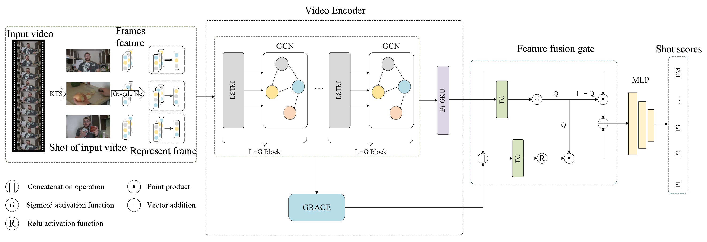
As shown in Figure 2, this article proposes a video summarization network based on dynamic graph contrastive learning and feature fusion, which is used to reduce the redundant information of the graph structure, improve the representation ability of the graph, and capture the semantic relationship between shots. The model mainly consists of three modules: feature extraction, video encoder, and feature fusion. For feature extraction, we first extract features from video frames and then select representative frames as the features of the shots. A representative frame of each shot is used as the node in the graph, and the graph structure is dynamically constructed according to the similarity between nodes. In the video encoder, the L-G Block is used to learn the temporal context and graph structure features between shots. Subsequently, the graph structures with different contexts are constructed, and the node features of the graph structures are optimized through graph contrastive learning, thus optimizing the graph structures and reducing the interference of redundant information. Finally, the weights of the shallow-level and deep-level features are dynamically adjusted through the feature fusion gate to achieve feature fusion, and the importance score of the shot is predicted by the fusion features.
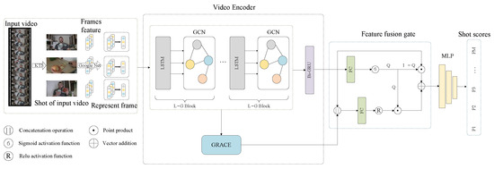
Figure 2.
Network architecture for video summarization generation based on dynamic graph contrastive learning and feature fusion.
3.1. Feature Extraction
The original video is defined as , , where denotes the n-th frame of the video; N denotes the total number of frames in the video; w and h represent the width and height of each image frame in pixels, respectively; and 3 denotes the number of channels of the image. The KTS algorithm [22] is used to segment the original video into short shots, and the set of video shots is denoted as , , M denotes the total number of shots in the original video, and denotes that there are frames in the m-th shot and . The depth feature of each frame , is extracted by GoogLeNet [23], and D denotes the feature dimension of the frame.
3.2. Video Encoder
In the video summarization task, the features should have both local and global properties. Therefore, we use graph construction to process the features. A shot is a short sequence of consecutive frames, which are captured as a single shot and convey similar semantics, so the features extracted from each frame by GoogLeNet are usually similar. To construct the video graph structure, we select a representative frame from each shot as the graph node and calculate the average of the Euclidean norm between the frames in each shot and the rest of the frames. The frame with the lowest average is selected as the representative frame.
We take the shot’s representative frame as the graph node and obtain the set of graph node features . We take the GoogLeNet feature of the representative frame as the graph node feature and .
The fully connected edge structure is prone to cause redundant information to interfere with the aggregation of node features, and the sparse graph structure established based on the relationship between shots in the preprocessing stage cannot be effectively integrated into the learning of graph structure features. Therefore, we dynamically construct the graph structure during training to enable the model to learn the optimal node connection scheme, thereby better achieving the aggregation of node features. We measure the similarity between graph nodes as the basis for establishing edge connections. Yasir et al. [24] proved that the cosine similarity is more suitable for describing the similarity between nodes, so we choose the cosine similarity as the description of the similarity between node and node .
When the cosine similarity exceeds the threshold , an edge is established between the two nodes, and is assigned as the weight of the edge, thus constructing the edge set E and the adjacency matrix A.
GCN is good at handling graph structured data and can effectively perform information propagation and feature extraction on graphs. Video shots also have certain temporal context relationships, and LSTM performs well in processing sequential data and can capture long-term dependencies in sequences. Therefore, we combine the two to form the L-G Block. LSTM performs information propagation and processing on the time sequence, and GCN performs information propagation on the graph structure. In the video encoder, by stacking L-G Blocks, the temporal context-enhanced features output from LSTM are fed into GCN, while the graph structure-enhanced features output from GCN are able to be fed into LSTM, thus taking advantage of the complementary strengths of LSTM and GCN for a better understanding of the correlations and patterns in the data. The input to the first layer of the L-G Block is the GoogLeNet features G. The forward propagation of the stacked layer of the L-G Block is as follows:
where Z denotes the number of layers of GCN, denotes the learnable weight matrix of the n-th layer, denotes the feature of the j-th node in the n-th layer of GCN. denotes the Laplacian matrix computed from the adjacency matrix A, and denotes the ReLU activation function.
3.3. Graph Contrastive Learning
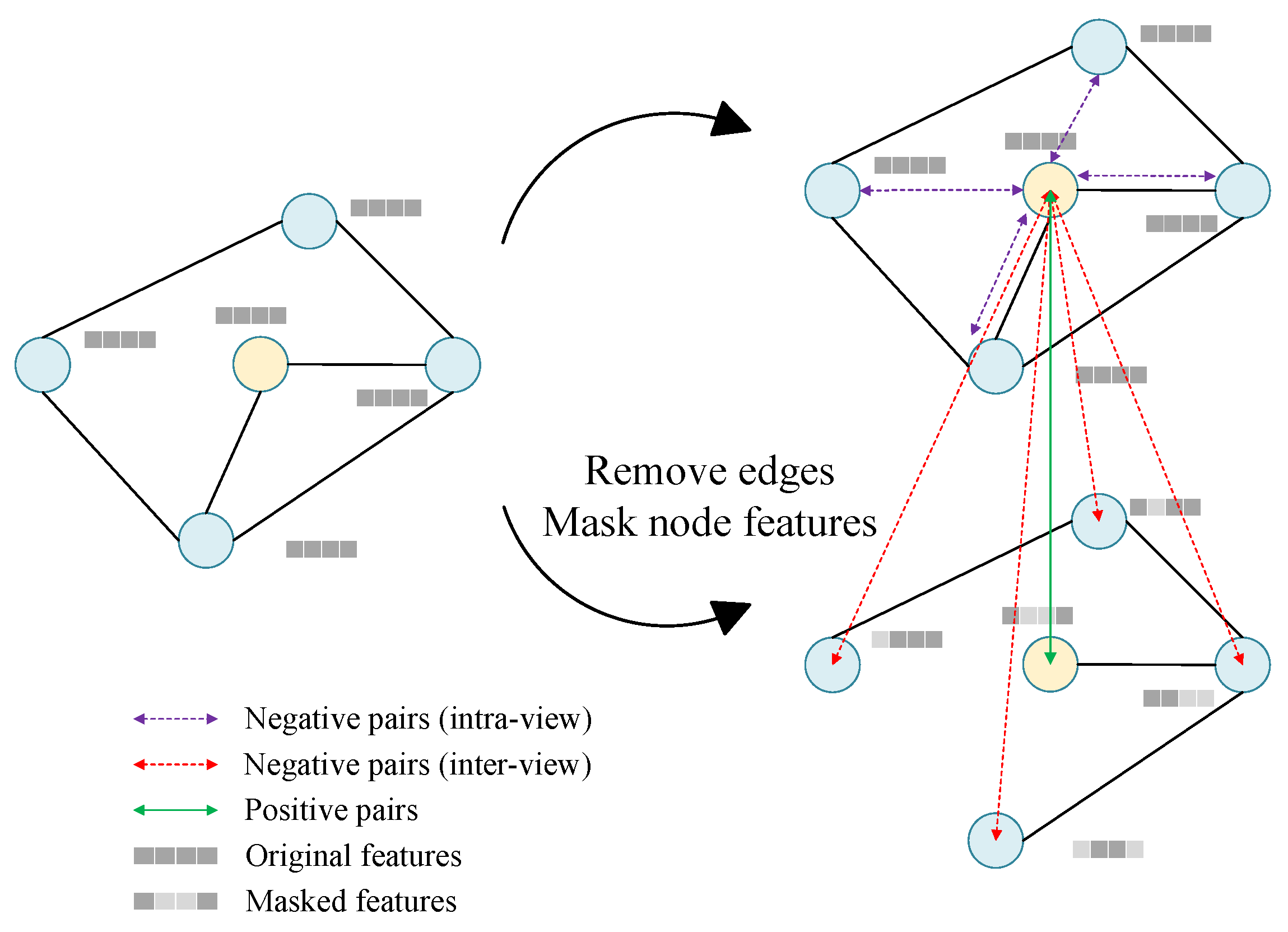
We use graph contrastive learning to optimize the graph structure by modifying the graph at both the structure and attribute levels, thus constructing graph views with different contexts. By maximizing the consistency of the representation of the same data in different graph views, we reduce the interference of redundant information and achieve the optimization of graph structure, thereby enhancing the learning effect. Specifically, as shown in Figure 3, in the GRACE module, two graph views , are generated at each iteration, then we input and into the GCN to capture the relationships between nodes and the internal features of nodes, and output the embedding representations of nodes , . During the iteration process, the model can learn the more optimal embedding representation of nodes, which can effectively eliminate the redundant and incorrect connections in the original graph structure.
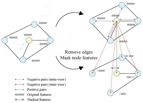
Figure 3.
Graph construction in graph contrastive learning.
Generating graph views is a key component of graph contrastive learning. For the generation of graph views and , retains the original graph structure and input features, and is generated by removing edges and masking features. For the node feature matrix of , Random positions of the feature matrix X are set to 0 according to a certain ratio. Specifically, a feature vector , is constructed following the Bernoulli distribution with probability , and the node features of can be denoted as
where denotes the connect operation, and ⊙ denotes the Hadmard product. We can obtain the adjacency matrix of graph by randomly removing edges of G. We sample a random mask matrix , from the Bernoulli distribution, where denotes the probability of each edge being removed, and the resulting adjacency matrix can be denoted as
3.4. Feature Fusion
After the above procedures, we obtain the output features of the dynamic graph X and the output features optimized by graph contrastive learning . The feature hierarchy of is higher and the semantic information is more abstract; the feature hierarchy of X is lower, and it mainly consists of perceptual features, but the feature information is more detailed. In order to retain key information from both shallow and deep features and remove redundant information which is irrelevant to the task, we designed a fusion gate mechanism, which dynamically controls the weight ratio of the two features through a gate control mechanism and fuses the two features. First, we input X to Bi-GRU to enhance its temporal features and obtain the feature . In order to ensure that the overall information of the two features is taken into account when deciding the gate control weights, we fuse feature C and through a cascaded manner and map the cascaded feature to the fusion feature space to obtain the fusion feature h:
The fusion feature contains deep-level features and shallow-level perceptual features of the video. By computing the gate control score based on the fusion feature, the model can learn from a richer feature space, which can help to extract more effective information for better integration of more information to regulate feature selection and optimize the complementarity and synergy between features:
where and are all learnable parameter matrices and and are learnable bias vectors. By regulating the weight of features through the gate control score Q, we obtain the final fusion feature :
Finally, the final fusion feature is input into the MLP to calculate the prediction score of the shot , which is used to evaluate the importance of the video shot.
3.5. Loss Function
In graph contrastive learning, we use the contrastive loss function, which maximizes the mutual information between input samples based on the maximum mutual information, thereby maximizing the similarity between positive samples and minimizing the similarity between negative samples. For any two node features and of and , the contrastive loss is as follows:
where denotes the normalized dot product between and . N denotes the total number of samples, and T denotes the temperature parameter used to control the smoothness of the maximum.
We use the MSE loss function to calculate the difference between the predicted and true values. The MSE loss function is mainly used for regression tasks and aims to minimize the sum of the squared errors between the predicted and true values, which can help the model make more accurate predictions for continuous numerical values.
where denotes the true score of the shot, and denotes the predicted score of the shot.
4. Experiments
4.1. Dataset
In this experiment, we used TVSum [25] and SumMe [26], two widely used video datasets in the video summarization field.
The TVSum dataset consists of 50 videos collected from YouTube, covering a variety of topics such as news reports, sports events, documentaries, and tutorials. The length of each video ranges from 2 to 10 min. The shortest video is 83 s and the longest video is 647 s, with an average length of 235 s. Each video is watched by 20 different users, who assign importance scores to each video frame at each time point, with a rating range of 1 to 5, where 5 indicates extremely important. The final score is derived from the ratings of all users.
The SumMe dataset includes 25 videos, covering sports activities, events, documentaries and user-generated content, with video lengths varying from a few minutes to several minutes. The shortest video is 32 s and the longest is 324 s, with an average length of 146 s. Each video contains frame-level importance ratings from 15 to 18 different users, with 0 indicating important and 1 indicating unimportant.
Both TVSum and SumMe datasets provide frame-level rating information. In video editing, a shot consists of a series of consecutive frames, and within the same shot, the video content tends to change less. To create a video summarization based on the shot scores, we use the kernel temporal segmentation (KTS) algorithm to segment the videos into shots so that each shot could be assigned corresponding scores. Based on these scores, we generate the final video summarization by using the 0/1 knapsack algorithm.
4.2. Experiment Setting
In the experiment, the entire dataset is first divided into a training set and a test set at a ratio of 80% to 20%. In order to improve the generalization of the experimental results, we randomly divide the data K times, perform K-fold cross-validation, and calculate the average of the K results as the final experimental results, K = 5. We set the learning rate to 0.006 and use Adam as the optimizer. The GRU is configured to be bidirectional with two layers, and the LSTM is set to be bidirectional with two layers. Additionally, the number of stacked layers in the L-G Block is two.
4.3. Evaluation of Indicators
The most commonly used evaluation indicator in video summarization studies is the F1 score, which needs to be calculated by Precision and Recall. Precision indicates the proportion of samples predicted by the model to be positive that are actually positive; Recall indicates the proportion of samples that the model is able to predict to be positive out of all the samples that are actually positive.
where N_match is the sum of the number of summary frames that can be matched between the truth summary frames and the generated summary frames, and N_extract is the number of generated summary frames.
where N_US is the number of truth value video summarization frames.
4.4. Comparative Experiments
Table 1 presents a comparison of our method with other state-of-the-art methods in terms of F1 score on the TVSum and SumMe datasets. vsLSTM [27] and dppLSTM [27] introduce a point process to enhance the performance of LSTM, facilitating the acquisition of diversified results based on global video context. DR-DSN [28] designed a deep summarization network for video summarization and proposed an end-to-end framework based on reinforcement learning, achieving more representative and diverse summaries by designing different reward functions. SUM-GAN [29] proposed a generative adversarial framework consisting of a summarizer and a discriminator, where the summarizer is an autoencoding long short-term memory network used for summarization generation, while the discriminator is responsible for identifying summarization videos from the original ones. SF-CVS [30] proposed a framework for motion-based video summarization, segmenting video streams into shots using transition detection and introducing self-attention to select key frames within shots. RSGN [9] encodes frames and shots hierarchically into sequences and graphs, where frame-level dependencies are captured by LSTM encoding and shot-level dependencies are captured by GCN, summarizing videos by leveraging both local and global dependencies between shots. GATVS [10] employed a novel spatial attention model, utilizing GAT to transform visual features of images into higher-level features and then combining them with semantic features processed by Bi-LSTM to select key frames. VJMHT [31] proposed a hierarchical transformer to aggregate shot information in videos, considering not only the internal structure of videos but also their global dependency relationships. 3DST-UNet [32] utilized spatiotemporal features for video summarization, combining reinforcement learning with 3DSTUNet to encode both spatial and temporal information of videos simultaneously. AoA [33] introduced a deep model based on a multi-attention module, including spatial, channel, and multi-head attention, enabling effective capture of feature relationships between spatial locations and channels.

Table 1.
Comparison with existing state-of-the-art methods on F1 score.
As shown in Table 1, compared to the existing vsLSTM and DPP-LSTM methods, our method achieves a higher F1 score on both datasets. This is because our method not only extracts temporal features but also effectively captures structural features within the videos. Compared to the DR-DSN, SUM-GAN, SF-CVS, 3DST-Unet, and AoA methods, our method outperforms them on both datasets. This can be attributed to the alternating extraction of temporal and structural features in our method, along with feature optimization using graph contrastive learning. On the TVSum dataset, our method outperforms RSGN by 0.2%, and on the SumMe dataset, it surpasses by 6.5%. This is attributed to the more efficient extraction of temporal and structural features in our method. Compared to GATVS, our method achieves a 1.2% improvement on the TVSum dataset and remains comparable on the SumMe dataset. This may be due to the feature optimization using graph contrastive learning and the comprehensive integration of features through gate mechanisms in our method. In comparison to VJMHT, our method slightly trails behind on the TVSum dataset, while on the SumMe dataset, it outperforms VJMHT by 0.9%. This is possibly because VJMHT effectively extracts temporal features using hierarchical transformers, particularly suitable for longer videos like those in the TVSum dataset. Meanwhile, our method considers both temporal and structural features, hence performing better on the SumMe dataset.
4.5. Ablation Experiments
In order to investigate the impact of key components in the model on its performance, we conducted three ablation experiments on two datasets. We designed three ablation experiments on two datasets: ablation on dynamic graph contrastive learning, feature fusion, and the number of stacked layers of L-G Blocks. In the ablation experiment of dynamic graph contrastive learning, CG_model removes the design of dynamic graphs, uses the features extracted by GoogleNet as the input features of the graph contrastive learning module, and utilizes the features extracted by GoogleNet to fuse with the output features of the graph contrastive learning module in the feature fusion; DG_model removes the graph contrastive learning module and utilizes GoogleNet features and L-G Blocks features as input to the feature fusion module; SG_model uses a static graph instead of a dynamic graph. As shown in Table 2, the performance of CG_model is lower than that of DGC-FNet under both datasets, indicating that the dynamic graph setting can effectively enhance the model’s ability to learn the graph structure data. Meanwhile, SG_model has a better performance under the TVSum dataset, which indicates that studying the graph structure before graph contrastive learning is beneficial for model learning. The performance of DG_model under the TVSum and SumMe datasets is lower than the performance of each of the other models, indicating that graph contrastive learning can reduce the influence of redundant information and enhance the model’s ability to represent the features of graph structure data.
Table 2.
Comparison of dynamic graph contrastive learning ablation experiments on F1 score.
In the feature fusion ablation experiments, CON_Fusion does not perform the fusion of shallow-level features and deep-level features and directly inputs the features from the graph contrastive learning module into the MLP; CRO_Fusion uses cross-attention fusion of the features from the L-G Blocks and the features from the graph contrastive learning module; CAT_Fusion fuses the features output by the L-G Blocks and the features output by the graph contrastive learning module by means of vector concatenation. As shown in Table 3, the performance of CRO_Fusion is lower than other fusion methods, indicating that the two features do not need to be semantically feature-wise aligned and their relationship should be complementary in nature. CON_Fusion performs poorly without performing feature fusion, suggesting that utilizing the complementary strengths of different features in semantic representation facilitates the model to represent the semantic features of the data more and more comprehensively.
Table 3.
Comparison of feature fusion ablation experiments on F1 score.
In the ablation experiments of combining the number of stacked layers of L-G Blocks, as shown in Table 4, the model with the number of stacked layers of two performs the best on both datasets, indicating that the stacking of the number of layers of LSTM and GCN can help the model to take care of both the graph data and the learning of long term dependencies, but too many layers may lead to the occurrence of the problem of overfitting, which will degrade the performance of the model.
Table 4.
Comparison of the number of stacked layers of L-G blocks ablation experiments on F1 score.
4.6. Visualization Result
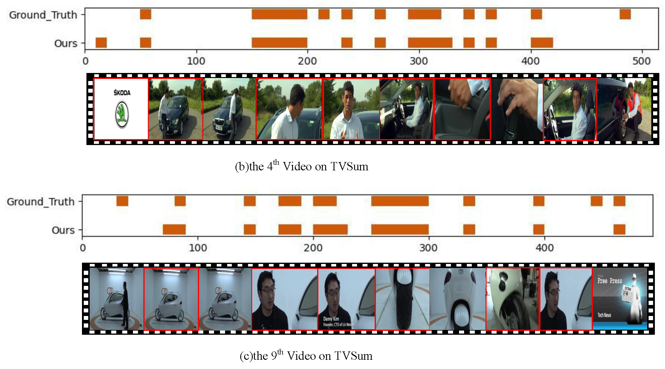
In the visualization experiments, the summaries generated by our proposed model were compared with the ground truth to evaluate the quality of the generated summaries. The video examples shown in Figure 4 are from the 16th video in SumMe and the 4th and 9th videos in TVSum. Among them, the ground truth video summarization in SumMe are sparse, and the ground truth video summarization in TVSum are denser. The visualization experiments comparison revealed that the summaries generated by our model were very close to the ground truth and could accurately select the representative frames, which indicated that the DGC-FNet was able to adapt better to the task of generating video summarization in different scenarios.
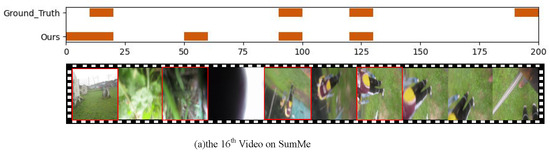

Figure 4.
Visualization experiments comparison of model-generated summaries and ground truth.
5. Conclusions
This article presents a video summarization generation network based on dynamic graph contrastive learning and feature fusion. The purpose is to fully capture the sequential temporal context and graph structural data features by leveraging the advantages of combining LSTM and GCN. Through dynamic graph contrastive learning, redundant information in the graph is reduced, enhancing the graph’s representational capacity and enabling the model to capture key information more accurately within the graph. We first segment the video into shots and select the features of representative frames as the features of the current shot. Then, the L-G Block is utilized to learn both the temporal context features of the sequence and the structural features of the graph, optimizing the graph structure through graph contrastive learning to enhance its representational capacity and reduce redundancy. The temporal context features of sequences and graph structure features are learned through the L-G Block, and the graph structure is optimized using graph contrastive learning, thus enhancing the graph representation and reducing redundancy. Finally, the fusion of the shallow-level feature output through L-G blocks, the deep-level feature output through graph contrastive learning, and the weights of the two are dynamically adjusted through the gating mechanism, thus achieving feature fusion and effectively avoiding the loss of key information.
In future research, we plan to incorporate multimodal information into video summarization, such as visual, audio, and text data, to generate more accurate and targeted video summarization. Additionally, to enable users to understand the inference process of the model and understand why certain content is selected for summarization, we will explore methods to improve the interpretability of the video summarization model.
Author Contributions
Conceptualization, G.W.; methodology, J.Z.; software, X.B. and Y.C.; writing—original draft preparation, J.Z.; writing—review and editing, J.Z. All authors have read and agreed to the published version of the manuscript.
Funding
This research was funded by Natural Science Foundation of Gansu Province grant number 21JR7RA570, 20JR10RA334; Basic Research Program of Gansu Province grant number 22JR11RA106; Gansu University of Political Science and Law Major Scientific Research and Innovation Projects grant number GZF2020XZDA03; the Young Doctoral Fund Project of Higher Education Institutions in Gansu Province in 2022 grant number 2022QB-123; Gansu Province Higher Education Innovation Fund Project grant number 2022A-097; the University-level research funding project grant number GZFXQNLW022; University-level Innovative Research Team of Gansu University of Political Science and Law.
Data Availability Statement
Dataset available on request from the authors.
Conflicts of Interest
The authors declare no conflicts of interest. The funders had no role in the design of the study; in the collection, analyses, or interpretation of data; in the writing of the manuscript; or in the decision to publish the results.
References
- Saini, P.; Kumar, K.; Kashid, S.; Saini, A.; Negi, A. Video summarization using deep learning techniques: A detailed analysis and investigation. Artif. Intell. Rev. 2023, 56, 12347–12385. [Google Scholar] [CrossRef] [PubMed]
- Xu, W.; Wang, R.; Guo, X.; Li, S.; Ma, Q.; Zhao, Y.; Guo, S.; Zhu, Z.; Yan, J. Mhscnet: A multimodal hierarchical shot-aware convolutional network for video summarization. In Proceedings of the ICASSP 2023—2023 IEEE International Conference on Acoustics, Speech and Signal Processing (ICASSP), Rhodes Island, Greece, 4–10 June 2023; pp. 1–5. [Google Scholar]
- Wu, J.; Zhong, S.H.; Liu, Y. MvsGCN: A novel graph convolutional network for multi-video summarization. In Proceedings of the 27th ACM International Conference on Multimedia, Nice, France, 21–25 October 2019; pp. 827–835. [Google Scholar]
- Meena, P.; Kumar, H.; Yadav, S.K. A review on video summarization techniques. Eng. Appl. Artif. Intell. 2023, 118, 105667. [Google Scholar] [CrossRef]
- Zhao, B.; Li, X.; Lu, X. Hsa-rnn: Hierarchical structure-adaptive rnn for video summarization. In Proceedings of the IEEE Conference on Computer Vision and Pattern Recognition, Salt Lake City, UT, USA, 18–23 June 2018; pp. 7405–7414. [Google Scholar]
- Zhao, B.; Li, X.; Lu, X. TTH-RNN: Tensor-train hierarchical recurrent neural network for video summarization. IEEE Trans. Ind. Electron. 2020, 68, 3629–3637. [Google Scholar] [CrossRef]
- Haq, H.M.U.; Asif, M.; Ahmad, M.B. Video Summarization Techniques: A Review. Int. J. Sci. Technol. Res. 2020, 9, 146–153. [Google Scholar]
- Zhou, J.; Cui, G.; Hu, S.; Zhang, Z.; Yang, C.; Liu, Z.; Wang, L.; Li, C.; Sun, M. Graph neural networks: A review of methods and applications. AI Open 2020, 1, 57–81. [Google Scholar] [CrossRef]
- Zhao, B.; Li, H.; Lu, X.; Li, X. Reconstructive sequence-graph network for video summarization. IEEE Trans. Pattern Anal. Mach. Intell. 2021, 44, 2793–2801. [Google Scholar] [CrossRef] [PubMed]
- Zhong, R.; Wang, R.; Zou, Y.; Hong, Z.; Hu, M. Graph attention networks adjusted bi-LSTM for video summarization. IEEE Signal Process. Lett. 2021, 28, 663–667. [Google Scholar] [CrossRef]
- Zhu, W.; Han, Y.; Lu, J.; Zhou, J. Relational reasoning over spatial-temporal graphs for video summarization. IEEE Trans. Image Process. 2022, 31, 3017–3031. [Google Scholar] [CrossRef]
- Yuan, L.; Tay, F.E.H.; Li, P.; Feng, J. Unsupervised video summarization with cycle-consistent adversarial LSTM networks. IEEE Trans. Multimed. 2019, 22, 2711–2722. [Google Scholar] [CrossRef]
- Apostolidis, E.; Adamantidou, E.; Metsai, A.I.; Mezaris, V.; Patras, I. Video summarization using deep neural networks: A survey. Proc. IEEE 2021, 109, 1838–1863. [Google Scholar] [CrossRef]
- Sreeja, M.; Kovoor, B.C. A multi-stage deep adversarial network for video summarization with knowledge distillation. J. Ambient Intell. Humaniz. Comput. 2023, 14, 9823–9838. [Google Scholar] [CrossRef]
- Xiao, S.; Zhao, Z.; Zhang, Z.; Guan, Z.; Cai, D. Query-biased self-attentive network for query-focused video summarization. IEEE Trans. Image Process. 2020, 29, 5889–5899. [Google Scholar] [CrossRef] [PubMed]
- Lin, J.; Zhong, S.h.; Fares, A. Deep hierarchical LSTM networks with attention for video summarization. Comput. Electr. Eng. 2022, 97, 107618. [Google Scholar] [CrossRef]
- Kipf, T.N.; Welling, M. Semi-supervised classification with graph convolutional networks. arXiv 2016, arXiv:1609.02907. [Google Scholar]
- Wu, J.; Zhong, S.h.; Liu, Y. Dynamic graph convolutional network for multi-video summarization. Pattern Recognit. 2020, 107, 107382. [Google Scholar] [CrossRef]
- Veličković, P.; Fedus, W.; Hamilton, W.L.; Liò, P.; Bengio, Y.; Hjelm, R.D. Deep Graph Infomax. ICLR 2019, 2, 4. [Google Scholar]
- Zhu, Y.; Xu, Y.; Yu, F.; Liu, Q.; Wu, S.; Wang, L. Deep graph contrastive representation learning. arXiv 2020, arXiv:2006.04131. [Google Scholar]
- Li, W.; Qi, D.; Zhang, C.; Guo, J.; Yao, J. Video summarization based on mutual information and entropy sliding window method. Entropy 2020, 22, 1285. [Google Scholar] [CrossRef] [PubMed]
- Potapov, D.; Douze, M.; Harchaoui, Z.; Schmid, C. Category-specific video summarization. In Proceedings of the Computer Vision–ECCV 2014: 13th European Conference, Zurich, Switzerland, 6–12 September 2014; Proceedings, Part VI 13. Springer: Berlin/Heidelberg, Germany, 2014; pp. 540–555. [Google Scholar]
- Szegedy, C.; Liu, W.; Jia, Y.; Sermanet, P.; Reed, S.; Anguelov, D.; Erhan, D.; Vanhoucke, V.; Rabinovich, A. Going deeper with convolutions. In Proceedings of the IEEE Conference on Computer Vision and Pattern Recognition, Boston, MA, USA, 7–12 June 2015; pp. 1–9. [Google Scholar]
- Yasir, M.A.; Ali, Y.H. Dynamic background subtraction in video surveillance using color-histogram and fuzzy c-means algorithm with cosine similarity. Int. J. Online Biomed. Eng. 2022, 18, 74–85. [Google Scholar] [CrossRef]
- Song, Y.; Vallmitjana, J.; Stent, A.; Jaimes, A. Tvsum: Summarizing web videos using titles. In Proceedings of the IEEE Conference on Computer Vision and Pattern Recognition, Boston, MA, USA, 7–12 June 2015; pp. 5179–5187. [Google Scholar]
- Gygli, M.; Grabner, H.; Riemenschneider, H.; Van Gool, L. Creating summaries from user videos. In Proceedings of the Computer Vision–ECCV 2014: 13th European Conference, Zurich, Switzerland, 6–12 September 2014; Proceedings, Part VII 13. Springer: Berlin/Heidelberg, Germany, 2014; pp. 505–520. [Google Scholar]
- Zhang, K.; Chao, W.L.; Sha, F.; Grauman, K. Video summarization with long short-term memory. In Proceedings of the Computer Vision–ECCV 2016: 14th European Conference, Amsterdam, The Netherlands, 11–14 October 2016; Proceedings, Part VII 14. Springer: Berlin/Heidelberg, Germany, 2016; pp. 766–782. [Google Scholar]
- Zhou, K.; Qiao, Y.; Xiang, T. Deep reinforcement learning for unsupervised video summarization with diversity-representativeness reward. In Proceedings of the AAAI Conference on Artificial Intelligence, New Orleans, LA, USA, 2–7 February 2018; Volume 32. [Google Scholar]
- Mahasseni, B.; Lam, M.; Todorovic, S. Unsupervised video summarization with adversarial lstm networks. In Proceedings of the IEEE Conference on Computer Vision and Pattern Recognition, Honolulu, HI, USA, 21–26 July 2017; pp. 202–211. [Google Scholar]
- Huang, C.; Wang, H. A novel key-frames selection framework for comprehensive video summarization. IEEE Trans. Circuits Syst. Video Technol. 2019, 30, 577–589. [Google Scholar] [CrossRef]
- Li, H.; Ke, Q.; Gong, M.; Zhang, R. Video joint modelling based on hierarchical transformer for co-summarization. IEEE Trans. Pattern Anal. Mach. Intell. 2022, 45, 3904–3917. [Google Scholar] [CrossRef] [PubMed]
- Liu, T.; Meng, Q.; Huang, J.J.; Vlontzos, A.; Rueckert, D.; Kainz, B. Video summarization through reinforcement learning with a 3D spatio-temporal u-net. IEEE Trans. Image Process. 2022, 31, 1573–1586. [Google Scholar] [CrossRef] [PubMed]
- Puthige, I.; Hussain, T.; Gupta, S.; Agarwal, M. Attention over attention: An enhanced supervised video summarization approach. Procedia Comput. Sci. 2023, 218, 2359–2368. [Google Scholar] [CrossRef]

Disclaimer/Publisher’s Note: The statements, opinions and data contained in all publications are solely those of the individual author(s) and contributor(s) and not of MDPI and/or the editor(s). MDPI and/or the editor(s) disclaim responsibility for any injury to people or property resulting from any ideas, methods, instructions or products referred to in the content. |
© 2024 by the authors. Licensee MDPI, Basel, Switzerland. This article is an open access article distributed under the terms and conditions of the Creative Commons Attribution (CC BY) license (https://creativecommons.org/licenses/by/4.0/).