Speech Emotion Recognition Based on Temporal-Spatial Learnable Graph Convolutional Neural Network

Abstract

The Graph Convolutional Neural Networks (GCN) method has shown excellent performance in the field of deep learning, and using graphs to represent speech data is a computationally efficient and scalable approach. In order to enhance the adequacy of graph neural networks in extracting speech emotional features, this paper proposes a Temporal-Spatial Learnable Graph Convolutional Neural Network (TLGCNN) for speech emotion recognition. TLGCNN firstly utilizes the Open-SMILE toolkit to extract frame-level speech emotion features. Then, a bidirectional long short-term memory (Bi LSTM) network is used to process the long-term dependencies of speech features which can further extract deep frame-level emotion features. The extracted frame-level emotion features are then input into subsequent network through two pathways. Finally, one pathway constructs the extracted frame-level deep emotion feature vectors into a graph structure applying an adaptive adjacency matrix to catch latent spatial connections, while the other pathway concatenates emotion feature vectors with graph-level embedding obtained from learnable graph convolutional neural network for prediction and classification. Through these two pathways, TLGCNN can simultaneously obtain temporal speech emotional information through Bi-LSTM and spatial speech emotional information through Learnable Graph Convolutional Neural (LGCN) network. Experimental results demonstrate that this method achieves weighted accuracy of 66.82% and 58.35% on the IEMOCAP and MSP-IMPROV databases, respectively.

1. Introduction

Emotions are an indispensable part of human social interaction, and are of great significance for interpersonal communication, emotional health, psychological diagnosis, and medical care [1]. Traditionally, emotion recognition mainly relies on non-speech methods such as facial expressions, body language, and language. With the development and widespread application of speech technology, more and more emotional information can be obtained from speech signals [2]. Voice signals can transmit rich emotional information, including emotions, emotional states, and emotional tendencies. With the rapid development of speech technology, including natural language processing (NLP), speech synthesis, and speech recognition, the research on Speech Emotion Recognition (SER) [1] has also been rapidly developed. SER can help computers better understand users’ emotional states and needs, thereby improving the experience of human-computer interaction. For example, intelligent voice assistants can provide emotion-oriented services based on the user’s emotional preferences by recognizing their emotional state, making the interaction between the user and the computer more natural and intelligent [3]. SER can also be applied in the fields of emotional health and psychological diagnosis, helping psychologists and clinical doctors to more accurately evaluate the emotional state and mental health level of patients [4,5]. By analyzing the patient’s voice signals, objective emotional evaluation indicators can be provided to assist in psychological diagnosis and treatment processes. At the same time, SER can provide an objective and effective emotional assessment tool for research fields such as psychology and social sciences, reducing the subjectivity and objectivity of traditional emotional assessment methods, and helping to further study the role and impact of emotions in individual and social interactions [1]. Therefore, the study of SER has significant research and practical value.

Interpersonal emotional interactions encompass various modalities such as facial expression, text, gesture, and speech [6,7,8]. Among them, speech can directly reflect dynamic changes in emotions. Therefore, speech emotion recognition, as a real-time emotion recognition method, has attracted widespread attention. Currently, research on speech emotion recognition has made significant progress. In terms of feature extraction, researchers have proposed various effective methods, including rhythmic features such as energy, zero crossing rate and pitch frequency [9], musical quality features such as jitter and amplitude [10], and spectral features including Mel-frequency cepstral coefficients (MFCCs), Linear Prediction Coefficients (LPCs), Linear Prediction Cepstral Coefficients (LPCCs), etc. [11]. These features capture information relevant to emotions in speech signals, providing input for a subsequent emotion recognition model. In recent years, with the advancement of deep learning, many researchers have begun to utilize neural networks for feature extraction from speech samples. For example, Convolutional Neural Network (CNN) [12,13], Recurrent Neural Network (RNN) [14], Long Short-Term Memory (LSTM) network [15,16]. Later, neural networks based on CNN and RNN and their corresponding improved neural networks Convolutional Recurrent Neural Network (CRNN) [17], and CNN-LSTM [18] are commonly used as model framework. However, with the increase in the number of input speech samples and higher requirements for recognition effects, and deeper convolution operations, these methods have higher computational costs and are difficult to optimize. In addition, the attention mechanism is introduced into the SER task [19], which allows the model to focus more on key features related to emotion in the speech signal, helps extract and utilize key information, and improves model robustness. But its huge computational complexity degree often leads to reduced efficiency, and too many model parameters may lead to the risk of overfitting.

In recent years, GCN has demonstrated significant research and practical value in biomedicine [20], predictive medicine [21], traffic forecast [22], etc. Using GCN to handle speech emotion recognition tasks is a new way to enter the field of speech emotion recognition. The GCN model structure parameters are small and therefore more efficient. Using GCN to handle SER tasks is considered an efficient and scalable way [23]. The graph model networks can simultaneously solve Euclidean structure and non-Euclidean structure data. GCN can better learn the complex relationships between nodes. Shirian et al. [23] employed graph structure to handle speech emotion recognition. They use predefined a linear graph structure and a cyclic graph structure to embed the extracted speech features into nodes in the graph structure and use graph convolutional neural networks for training. The model achieved good performance and the number of training parameters was significantly reduced. Liu et al. [24] proposed constructing graphs from utterances of different lengths and use frames as nodes to embed SER in the graph. They compared different graph convolutional networks (GCNs) to handle the SER problem in a graph classification manner and discussed several different pooling methods on obtaining graph-level embeddings.

Using graphs to model speech faces two challenges. One is how to define the graph structure of speech data. The other is that GCN may not be as interpretable as traditional feature extraction and classification methods for speech emotion recognition tasks, which may reduce understanding of model decision-making processes. This suggests that additional feature extraction steps may be required to convert the speech data into graph data suitable for input into the GCN. The way of defining graph structure in GCN is generally divided into three categories, namely, static graph structure, dynamic graph structure and adaptive graph structure. The static graph structure refers to the use of a predefined adjacency matrix during training [25]. Dynamic graph structure [26] and adaptive graph structure [27] can dynamically change the connection relationships and weights of nodes in the graph. Dynamic graph structure updates node connections and weights with certain temporal information [26], while adaptive graph structure [27] updates node connections and weights based on node features or features learned from data. Some scholars combine GCN with other networks to improve the accuracy of GCN for SER tasks. Su et al. [28] proposed a graph attention bidirectional gated recurrent neural network (GA-GRU). They applied a graph attention mechanism on the bidirectional gated recurrent unit network (Bi-GRU) to improve speech emotion recognition (SER) accuracy. The GA-GRU combines speech modeling of long-range time series and uses graph structures to further enhance the complex modeling of emotional modulation. Liu et al. [29] used the space-based graph isomorphism network (GIN); they applied LSTM + five-layer GIN network, and then applied the output function in each GIN layer to obtain a graph-level embedding, in which the graph structure was obtained by aggregating neighbor nodes.

Using GCN can solve the limitations of complex models that are difficult to optimize. In order to make GCN deeply understand the speech emotion classification problem, the temporal features are first modeled and extracted first and then the extracted results are embedded in the graph. In order to obtain a graph structure that is more suitable for speech data, inspired by [23,27,28,29], this paper proposes a Temporal-Spatial Learnable Graph Convolutional Neural Network (TLGCNN) for speech emotion recognition. TLGCNN comprises the Bi-directional Long Short-Term Memory (Bi-LSTM) layer, the Learnable Graph Convolutional Neural (LGCN) layer, and the prediction layer. The Bi-LSTM layer employs Bi-LSTM and frame smoothing components to capture temporal dependencies. Continuity features are an important characteristic of speech samples, and Bi-LSTM [30] can leverage information from preceding and subsequent contexts in input sequences, enabling a more accurate understanding of semantics and structure within sequences, capturing long-term dependencies and contextual information, which is effective for speech emotion recognition tasks. The temporal dependencies between different frames of speech sample data in the database may affect emotion classification. Therefore, TLGCNN applies Bi-LSTM and frame smoothing components to handle potential impact weights among the most discriminative frame nodes. The Bi-LSTM layer extracts raw features for each speech sample, capturing long-term dependencies by employing Bi-LSTM and obtaining deep frame-level features. The LGCN layer applies an adaptive adjacency matrix to capture spatial dependencies. Using the GCN methodology introduces a graph-based approach to the field of speech emotion recognition. Compared to other methods, GCN effectively leverages graph and node features to learn node representations, thereby achieving a better performance. The adaptive adjacency matrix automatically generates spatial relationships based on the characteristics of speech data, evolving with network training to match node connections for emotion recognition tasks. The LGCN layer employs an adaptive adjacency matrix and two layers of GCN. It embeds deep frame-level feature vectors into nodes, constructing a set of graph structure features. After LGCN training, the graph structure features enter the pooling layer to obtain graph-level embedded speech spatial emotion features. The prediction layer concatenates temporal emotion features (deep frame-level features) and spatial emotion features for prediction and classification. Therefore, through the aforementioned three-layer network architecture, TLGCNN can simultaneously extract effective speech emotion features in both temporal and spatial domains, addressing the task of speech emotion recognition.

The remaining structure of this article is outlined as follows. The second section elaborates on the proposed network model, while the third section delineates the experimental setup and datasets employed, presenting the evaluation of experimental data and analysis of results. Finally, there is the summary section of the paper.

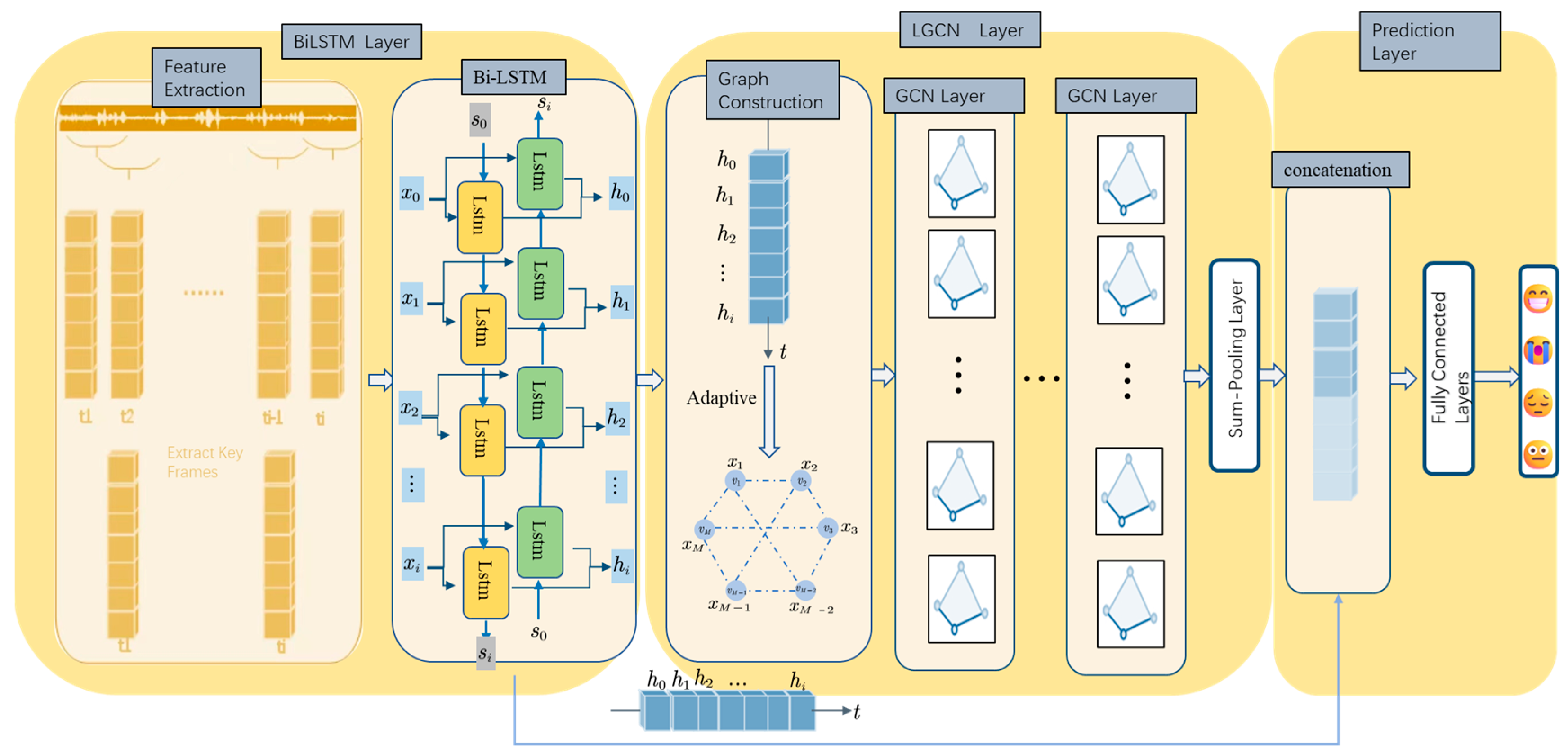
2. Temporal-Spatial Learnable Graph Convolutional Neural Network

This section introduces the proposed Temporal-Spatial Learnable Graph Convolutional Neural Network (TLGCNN) for speech emotion recognition, which is illustrated in Figure 1. TLGCNN comprises the Bi-LSTM layer, the LGCN layer, and the prediction layer. The Bi-LSTM layer is divided into feature extraction, frame smoothing components, and Bi-LSTM. Firstly, for each speech sample, frame segmentation, windowing, and padding are performed using the Open-SMILE-2.3.0 toolkit [31] to obtain frame-level emotion features $x_t$. These features are then smoothed using a K-means smoothing component, with averaging performed on every $K$ frames. Subsequently, the averaged frame-level emotion feature vectors undergo Bi-LSTM to extract temporal feature information, generating deep frame-level emotion feature vectors $h_t$. The LGCN layer consists of two GCN layers and a pooling layer. Similar to literature [23], we model each deep frame-level emotion feature vector as a frame-level graph structure. Then, we embed the deep frame-level emotion feature vectors $h_t$ of each speech signal into the nodes of each graph. The resulting set of graph structure feature vectors $g_n$ is inputted into the LGCN layer. The LGCN layer utilizes an adaptive adjacency matrix [27] to capture spatial dependencies between nodes and trains parameters using two GCN layers. Similar to prior works [23,32], the LGCN layer employs a sum pooling layer to convert node classification tasks into graph classification tasks. The prediction layer comprises a feature concatenation layer, a fully connected layer, and a softmax function. The feature concatenation layer combines temporal-dependent deep frame-level emotion feature vectors $h_t$ with spatial-dependent graph classification features $g_i$. A fully connected layer and the softmax function are then used for prediction classification.

2.1. Feature Extraction

Various tools can be employed for extracting speech emotion features. Open-Smile, as an open-source speech analysis toolkit which has rich feature extraction capabilities, cross platform capabilities, and flexibility, is the most widely used tool for speech emotion recognition. We use the Open-SMILE open-source toolkit [31] and use the feature set from the Interspeech 2009 emotion challenge [33]. This feature set comprises 384 features computed by applying statistical functions to Low-Level Descriptors (LLDs), including MFCCs, zero crossing rate, jitter, fundamental frequency, and frame energy. These features basically include all characteristics of speech.

To enhance the emotional content within each speech sample and improve model recognition performance, we employ a sliding window of 25 ms length with a step size of 10 ms to locally extract LLDs from each speech sample. A moving average filter is then applied to smooth each extracted feature, and first-order delta coefficients are computed. If the length of the speech sample is insufficient for the sliding window, padding is performed to ensure that each extracted frame feature has equal length, resulting in overlapping speech segments of 25 ms length [23].

2.2. Bi-LSTM

Speech signals constitute typical time series data, and the structure of Recurrent Neural Network (RNN) is well-suited for such data. Long Short-Term Memory (LSTM) networks [34] effectively addresses the problem of gradient vanishing or exploding during RNN training. The core of the LSTM model is the memory cell, which updates its state at each time step and controls information flow through various gates.

At each time step, Bidirectional LSTM (Bi-LSTM) [30] operates on input sequences bidirectionally, incorporating specific hidden states for forward and backward to process information in both directions. At each time step, the Bi-LSTM network concatenates the current input vector with forward and backward hidden states and outputs a synthesized hidden state. Bi-LSTM consists of forward and backward LSTM, and the final output is a simple stacking of the two LSTMs.

In this paper, $H$ memory cells are used in each direction of the LSTM to encode left and right sequence contexts to capture long-term sequential information in the speech signal. To obtain the most discriminative frames, the extracted original features are averaged over every $K$ frames. The averaged frame-level emotional features are then used as elements in the input sequence to the Bi-LSTM, and the output at each time step is as follows [30]:

$$\left\{\begin{array}{c}\overrightarrow{h_t}=\overrightarrow{LSTM(\overrightarrow{x_t},\overrightarrow{h_{t-1}})}\\ \overleftarrow{h_t}=\overleftarrow{LSTM(\overleftarrow{x_t},\overleftarrow{h_{t+1}})}\\ h_t=BiLSTM(x)=\left\{\overrightarrow{h_t},\overleftarrow{h_t}\right\}=\left\{\overrightarrow{h_1},\overrightarrow{h_2},\dots \overrightarrow{h_T},\overleftarrow{h_1},\overleftarrow{h_2},\dots \overleftarrow{h_T}\right\}\end{array}\right.$$

(1)

where $\overrightarrow{x_t}$ and $\overleftarrow{x_t}$ represent the forward and backward representation of the input features $f_t$ at time step $t$, $\overrightarrow{h_t}$ and $\overleftarrow{h_t}$ are the output vector of the forward and backward LSTM, respectively, and $h_t$ represents the output vector of the entire Bi-LSTM model at time step $t$. The input features $f_t$ are used as elements in the input sequence $\overrightarrow{x_t}$ and $\overleftarrow{x_t}$:

$$\left\{\begin{array}{c}\overrightarrow{x_t}=f_t\\ \overleftarrow{x_t}=f_{T-t-1}\end{array}\right.$$

(2)

The entire input sequence is denoted as $\left\{(\overrightarrow{x_1},\overleftarrow{x_1}),(\overrightarrow{x_2},\overleftarrow{x_2}),\dots ,(\overrightarrow{x_T},\overleftarrow{x_T})\right\}$, and finally, all output vectors $h_t\in {\mathbb{R}}^{T\times H}$ at each time step are used as deep emotional recognition features.

2.3. Learnable Graph Convolutional Neural (LGCN)

2.3.1. Graph Construction

First, the deep frame-level emotional feature matrix $h_t$ is constructed into a corresponding graph $G=\left(V,E\right),V\in {\left\{v_i\right\}}_{i=1}^M$ where $V$ and $E$ represent the set of $M$ nodes and the set of edges connecting these nodes, respectively. The adjacency matrix $A\in {\mathbb{R}}^{M\times M}$ is used to represent the connections between nodes, where each element $A_{ij}$ represents the weight of the connection between nodes $v_i$ and $v_j$. Then, each node $v_i$ is linked with a corresponding node feature vector $h_t\in {\mathbb{R}}^P$, where each node feature vector utilizes the deep frame-level emotional feature vector $h_t$. Meanwhile, the feature matrix of each graph composed of node feature vectors corresponds to $X\in {\mathbb{R}}^{M\times P}$, where $M$ represents the number of nodes, $P$ represents the dimensionality of each node’s feature vector, and the feature matrix is denoted as $h_t=BiLSTM(x)=\{\overrightarrow{h_t},\overleftarrow{h_t}\}$. The graph construction strategy includes embedding the obtained deep emotional feature vector into nodes and forming graph level embeddings through pooling layers. Each speech sample is converted into a graph $G_j$, and the entire dataset is traversed to obtain $\left\{G_1,\dots ,G_N\right\}$, with corresponding emotional labels $\left\{Y_1,\dots ,Y_N\right\}$.

2.3.2. Graph Convolutional Layer

Given the adjacency matrix $A$ of a pre-constructed graph, the Laplacian matrix $L=D-A$ is obtained, where $D\in {\mathbb{R}}^{n\times n}$ is the degree matrix of the graph with $D_{ii}={\sum }_j{A}_{ij}$, and $A$ is the adjacency matrix of the graph structure. Normalization of the Laplacian matrix $L$ yields $\mathcal{L}=D^{-\frac{1}{2}}L{D}^{\frac{1}{2}}=I_n-D^{-\frac{1}{2}}L{D}^{\frac{1}{2}}$, where $I_n$ is the identity matrix of order $n$. The features $\mathcal{L}$ are decomposed to obtain $\mathcal{L}=U\mathsf{\Lambda }{U}^{-1}$, where $\mathsf{\Lambda }$ is a diagonal matrix consisting of $n$ eigenvalues, $U=\left(u_0,\dots ,u_{n-1}\right)$ represents a matrix composed of eigenvectors corresponding to eigenvalues in the normalized Laplacian matrix. Our work is based on signal processing on graphs [35]. Assuming that the time domain signal is convolved with the convolution kernel, Equation (3) is obtained by Fourier transform and inverse transform [32,33]:

$$g \mathrm{\ast } x=F^{-1}\left(F\left(g\right)F\left(x\right)\right)=U\left(U^{T}g{U}^{T}x\right)$$

(3)

According to $U^{T}L=\mathsf{\Lambda }{U}^T$, $U^{T}g\left(L\right)$ can be regarded as the characteristic function $g_{\theta }\left(\mathsf{\Lambda }\right)$ of the Laplacian matrix $L$. Therefore, it is obtained that:

$$g \mathrm{\ast } x=U{g}_{\theta }{U}^{T}x$$

(4)

where $g_{\theta }=U^{T}g=diag({\theta }_0,\dots ,{\theta }_{n-1})$ is the diagonal matrix. In each graph convolution operation, the normalized Laplacian matrix $\mathcal{L}$ needs to undergo spectral decomposition to obtain feature vectors $U=\left(u_0,\dots ,u_{n-1}\right)$. Since the computation cost of $U$ is relatively high, the Chebyshev polynomial expansion is introduced to approximate the spectral domain graph convolution with the convolutional kernel:

$$g_{\theta }=g_{\theta }(\mathsf{\Lambda })\approx \sum _{i=0}^{k-1}{\theta }_i{F}_i(\tilde{\mathsf{\Lambda }})$$

(5)

where $\tilde{\Lambda }=2\mathsf{\Lambda }/{\lambda }_{max}-I_N$ (the objective is to normalize $\mathsf{\Lambda }$ to the range $\left[-\mathrm{1,1}\right]$), parameter $\theta$ represents the polynomial coefficients, and $\mathsf{\Lambda }$ is the matrix of eigenvalues obtained after the eigendecomposition of the Laplacian operator. Substituting Equation (5) into Equation (4) yields:

$$g \mathrm{\ast } x=U\sum _{i=0}^{k-1}{\theta }_i{F}_i(\tilde{\mathsf{\Lambda }})U^{T}x=\sum _{i=0}^{k-1}{\theta }_i{F}_i(\tilde{L})x$$

(6)

Here, $F_i\left(\tilde{L}\right)$ is the k-th order Chebyshev polynomial evaluated at the Laplacian operator $\tilde{L}=\frac{2L}{{\lambda }_{max}}-I_N$ [36]. This expression provides a polynomial approximation of the parameterized frequency response, reducing model complexity. The recursive formula for $F_i\left(\tilde{L}\right)$ is $F_i\left(\tilde{L}\right)=2\tilde{L}{F}_{i-1}\left(\tilde{L}\right)-F_{i-2}\left(\tilde{L}\right)$, while $F_0\left(\tilde{L}\right)=I$ and $F_1\left(\tilde{L}\right)=\tilde{L}$. The first-order Chebyshev polynomial can approximate this operation well [37]. Assuming $k=1$ and ${\lambda }_{max}=2$, then $\tilde{L}=L-I$. The Equation (6) is then transformed to [23,37]:

$$g \mathrm{\ast } x={\theta }_{0}x-{\theta }_1{D}^{-\frac{1}{2}}A{D}^{\frac{1}{2}}x$$

(7)

Let $\theta ={\theta }_0=-{\theta }_1$, we obtain the final graph convolutional single-layer output $y=\theta \left(I+D^{-\frac{1}{2}}A{D}^{\frac{1}{2}}\right)x$. To prevent gradient explosion, $I+D^{-\frac{1}{2}}A{D}^{\frac{1}{2}}$ is transformed to ${\tilde{D}}^{-\frac{1}{2}}\tilde{A}{\tilde{D}}^{-\frac{1}{2}}$ with $\tilde{A}=A+I_N \mathrm{and} {\tilde{D}}_{ii}=\sum _j{\tilde{A}}_{ij}$ [37]. Finally, $l$ layers of GCNs yield:

$$Y^{\left(l+1\right)}=\sigma \left({\tilde{D}}^{-\frac{1}{2}}\tilde{A}{\tilde{D}}^{-\frac{1}{2}}{Y}^l{\Theta }^l\right)$$

(8)

Here $Y^0=X$ and $\Theta \in {\mathbb{R}}^{P\times F}$ is a parameter matrix of $\theta$. Here, $\sigma$ represents the sigmoid activation function.

2.3.3. Adaptive Adjacency Matrix

When employing graph structures to handle emotion recognition tasks, each node feature corresponds to the features extracted from the samples. Regarding the connections between nodes, researchers typically manually construct adjacency matrices according to certain rules or predefine them. Busso et al. demonstrate through the study of various acoustic features that there are emotionally salient parts in speech samples [38], and the predefined graph structure fails to account for the connections between emotionally salient nodes and other nodes, merely considering those connected to their immediate predecessors and successors. To address this limitation, we employ an Adaptive Adjacency Matrix (AAM) [27] for GCN. The AAM is capable of automatically generating graph relationships based on the characteristics of the speech data, rather than predefined graph relationships. This type of graph relationship evolves with network training to automatically update node connections that are more suitable for emotion recognition tasks [27].

The AAM [27] is specifically initialized by first randomly initializing a learnable node embedding matrix $M_A\in {\mathbb{R}}^{M\times P}$, where each row of $M_A$ represents an embedding of a node, and $P$ denotes the dimensionality of the node embeddings. During the model training process, $M_A$ is updated based on the loss computed by the objective function and optimized using an optimizer, gradually approaching the optimal value from the random initial value to obtain more suitable node embedding representations. Then, the graph structure is defined through node similarity, where the calculation of node similarity is inferred by multiplying $M_A$ and $M_A^T$ to deduce the spatial dependencies between each pair of nodes. From this, the adaptive matrix $M_A\cdot M_A^T$ is obtained. Subsequently, it sends the matrix into the softmax function to obtain the normalized matrix. The specific computation is illustrated in Equation (9) [27]:

$${\tilde{D}}^{-\frac{1}{2}}\tilde{A}{\tilde{D}}^{-\frac{1}{2}}=softmax\left(ReLU\left(M_A\cdot M_A^T\right)\right)$$

(9)

Equation (9) does not generate $A$ or compute the Laplacian matrix. Instead, it substitutes the result for ${\tilde{D}}^{-\frac{1}{2}}\tilde{A}{\tilde{D}}^{-\frac{1}{2}}$, reducing the complexity and repetition of operations required for feature decomposition. During the training process, $M_A$ is automatically updated to learn the hidden connections between nodes, eventually yielding the adaptive adjacency matrix. Rewriting Equation (9), the final adaptive adjacency matrix corresponding to graph convolution iterations is presented as follows in Equation (10):

$$Y=\Theta \left(I_n+softmax\left(ReLU\left(M_A\cdot M_A^T\right)\right)\right)X$$

(10)

In Equation (10), $X$ represents the emotion feature matrix, $I_n$ represents the identity matrix, and $\Theta$ represents the polynomial coefficients.

2.3.4. Graph-Level Embedding

Since each graph structure $G$ in the set $\left\{{ G}_1,\dots ,G_N\right\}$ is derived from a speech sample, and each speech sample corresponds to a unique manually annotated emotion label, LGCN performs graph classification for each graph structure rather than node classification, which differs from most tasks handled using GCN. Due to the limitations of maximum pooling and average pooling in preserving underlying information about graph structures [32], LGCN adopts a sum pooling layer function to convert node-level embedding into graph-level embedding. This enables the realization of graph classification with the calculation formula as follows [23]:

$$y_g=sumpool\left(Y^k\right)=\sum _{i=1}^M{y}_i^{\left(k\right)}$$

(11)

The output depth frame-level emotion feature vector of Bi-LSTM is spliced with the features obtained through LGCN training, and finally the softmax function is used to predict and classify the speech emotion to obtain the final probability. Therefore, TLGCNN can extract effective speech emotion features in time and space at the same time and solve the speech emotion recognition task. The final output is as follows:

$$Y_i=softmax\left(y_g\oplus h_i\right)$$

(12)

3. Datasets, Experiments, and Analysis

3.1. Datasets

This section introduces the databases used in the speech emotion recognition experiments of this paper, including the IEMOCAP [39] and the MSP-IMPROV [40] database.

3.1.1. IEMOCAP Database

The IEMOCAP database is a multimodal emotion database collected by the Sail Laboratory of the University of Southern California, which contains facial movement, speech and text information. The database was recorded by 10 male and female actors in 2 ways: scripted and improvised performances, with a total duration of about 12 h. In this experiment, we chose to use the data from the improvised performance part because this part of the data can more truly reflect the actors. emotional state. The improvisation part included a total of five dialogues, each of which was performed by two professional actors, one male and one female, according to a given emotional category to ensure the diversity and richness of the data [39]. Finally, multiple annotators perform category annotation. The speech emotion types corresponding to each dialogue in the experiment are labeled according to the voting mechanism. That is, the emotion label with the most emotion types given by the annotators in a dialogue is the emotion label of the dialogue. To be consistent with previous experimental studies [23], the speech dataset we selected ultimately contains 4490 samples, including 1103 angry, 595 happy, 1708 neutral and 1084 sad instances.

3.1.2. MSP-IMPROV Database

The MSP-IMPROV dataset is a performance audiovisual emotion database used to explore emotional behavior during spontaneous binary improvisation. The database contains data from 6 dynamic emotion sessions (12 actors) with a total of approximately 7798 speech samples spanning over 9 h, including 792 angry samples, 3477 neutral samples, 885 sad samples, and 2644 happy samples [40]. The collector defines a hypothetical scene for each sentence, and two actors improvise and speak contextualized sentences in each scene, using a voting mechanism to annotate the emotional content. The recordings were collected in a single-wall speaker. The audio was recorded by two collar microphones. The signal was sampled at 48 kHz and 32-bit PCM. The video was recorded by a digital camera with a resolution of 29.97 frames/s [40]. The database was collected in four scenarios, namely, P, R, S and T, which correspond, respectively, to the spontaneous expression of the preparation process, the scene of reading the target sentence, the recording of improvised scene transitions and the scene of improvised scene reading of the target sentence [40]. To be consistent with previous experimental studies, the dataset finally contained 7798 speech samples.

3.2. Implementation Details

We set the number of cells $H$ in LSTM to 120. For LSTM 120 memory cells output sequence, we construct a graph with 120 nodes. And for 64 batch size, we embed it into a 64-dimensional space [23]. Throughout the experiment, we exclusively utilize the Adam optimizer (learning rate is 0.01 every 50 epochs and decay rate is 0.5), while employing a dropout layer of 0.2 [23]. To mitigate overfitting, this paper uses five-fold cross-validation to evaluate the performance of the model, dividing the data set into five approximately equal subsets. For each cross-validation, one of the subsets is used as the test set, and the remaining four subsets are used as the training set, and the verification is performed cyclically. Our computational infrastructure comprises a tower server running on the Ubuntu operating system. In the realm of deep learning, we utilize NVIDIA GTX1080Ti and A4000 GPUs and frameworks such as PyTorch-1.11.1 and Keras-2.3.1, operating on CUDA 11.0.

Our method performed baseline comparison experiments. Then, we conducted ablation experiments on LSTM, Bi-LSTM and adaptive adjacency matrix. We used Student’s t test to calculate p-values and confidence intervals for baseline comparison and ablation experiments to discuss statistical differences. To validate the performance of the proposed TLGCNN model, experiments are conducted and analyzed on two speech emotion databases (IEMOCAP and MSP-IMPROV). In the case of uneven distribution of samples in both databases, the analysis in this study primarily focuses on the confusion matrices, weighted accuracy (WA), and unweighted accuracy (UA) of various methods. The calculation method of each metric is as follows [41]:

$$WA=\frac{\sum _{i=1}^{N}T{P}_i}{\sum _{i=1}^{N}T{P}_i+F{P}_i}$$

(13)

$$UA=\frac{1}{N}\sum _{i=1}^N\frac{T{P}_i}{T{P}_i+F{P}_i}$$

(14)

$T{P}_i$ represents the number of accurate predictions for each category, and $F{P}_i$ represents the number of prediction errors for each category. WA and UA can better evaluate the performance of the model on different categories, especially when the gap in the number of samples between categories is large. At this time, the impact of quantitative imbalance between different categories on the model evaluation results can be avoided as much as possible. Another evaluation index is the confusion matrix, which represents the difference between the predicted value and the true value.

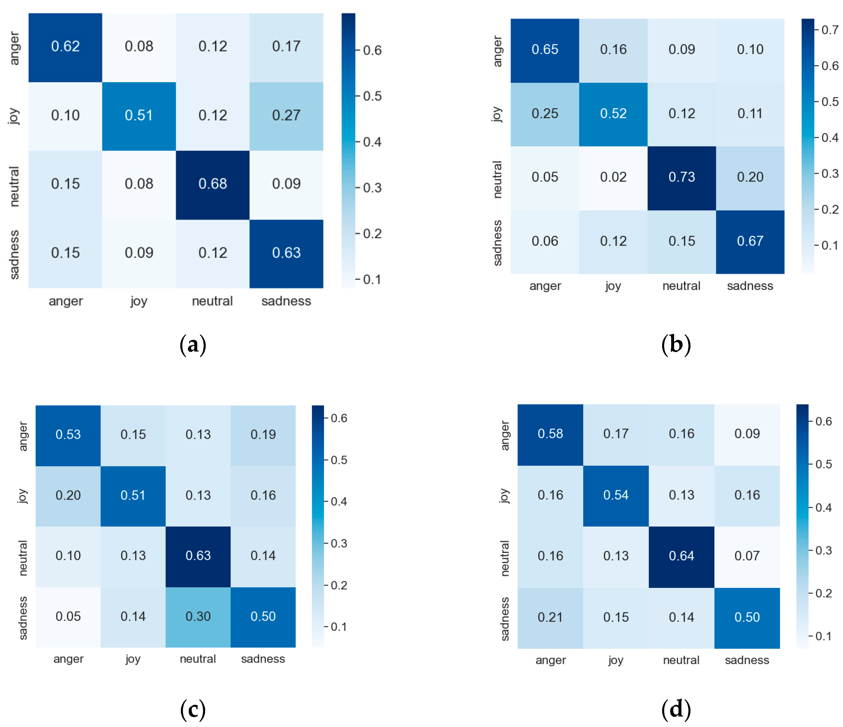
3.3. Results and Analysis

In order to assess the validity of our proposed TLGCNN, we summarize and evaluate the accuracy of the proposed TLGCNN in this paper and compare it to several methods in the field of speech emotion recognition in recent years. We discuss the performance comparison with baselines on two different datasets.

The GCN-2021 method [23] uses 384-dimensional emotional features extracted by the Open-SMILE toolkit, which are then input into the GCN module for further feature extraction and training. The GCN module uses undirected linear and cyclic graph structures, and finally predicts classification using sum-pooling, fully connected layers, and softmax functions.

The GA-GRU [28] method specifically utilizes emotional features extracted from speech samples by the Open-SMILE toolkit, which are then input into Bi-GRU. Subsequently, a graph attention mechanism is applied to enhance significant segments, which are then input into GCN for further feature extraction and training.

The GCN-2017 method [37] uses a standard form of spectral GCN for node classification. The architecture is tailored for node classification tasks, generating embeddings solely at the node level, while the method proposed in this paper is for graph classification, constructing a graph structure for each speech sample for prediction classification.

The LSTM-GIN method [29] uses a spatial graph isomorphism network based on the GIN network, applying LSTM + five-layer GIN network. Each GIN layer applies an output function to obtain graph-level embedding, aggregating neighboring nodes to obtain the graph structure.

The experimental results are shown in

Table 1. Speech emotion recognition results on IEMOCAP database.

IEMOCAP Database
Method	WA (%)	UA (%)
GA-GRU [28]	62.27	63.80
GCN-2021 [23]	64.25	61.15
LSTM-GIN [29]	64.65	65.53
GCN-2017 [37]	56.14	52.36
Attn-BLSTM [42]	59.33	49.96
RNN 2017 [19]	63.50	58.80
CRNN 2018 [17]	63.98	60.35
LSTM 2019 [16]	58.72	N/A
CNN-LSTM 2019 [16]	59.23	N/A
TLGCNN	66.82	64.21

and

Table 2. Speech emotion recognition results on MSP-IMPROV database.

MSP-IMPROV Database
Method	WA (%)	UA (%)
GA-GRU [28]	56.21	57.47
GCN-2021 [23]	56.24	54.32
GCN-2017 [37]	54.71	51.42
CNN 2019 [16]	50.84	N/A
LSTM 2019 [16]	51.21	N/A
CNN-LSTM 2019 [16]	52.36	N/A
TLGCNN	58.35	56.47

. N/A in the table indicates the lack of results for this indicator.

As shown in Table 1 and Table 2, the proposed TLGCNN outperforms other baseline models on the IEMOCAP database. The model achieves a Weighted Accuracy (WA) and Unweighted Accuracy (UA) of 66.82% and 64.21%, respectively. In experiments on the MSP-IMPROV database, the corresponding WA and UA are 58.35% and 56.47%, respectively, with only UA being approximately 1.00% lower than the GA-GRU method proposed by Su et al. [28]. The GA-GRU method assigns attention weights to frame segments, emphasizing the importance of frames with strong emotional content. TLGCNN surpasses the GCN-2021 method [21] by approximately 2.57% (p < 0.001, the confidence interval is (2.01, 2.95)) and 3.06% (p < 0.01, the confidence interval is (2.47, 3.52)) in WA and UA, respectively. The GCN-2021 method processes a higher number of frames per speech sample without averaging frame features, potentially leading to insufficient discriminatory information per frame. Moreover, it only utilizes emotional features extracted by the Open-SMILE toolkit as node features for training, which may not adequately represent emotional characteristics. Additionally, it lacks modeling of temporal dependencies and the predefined sequential graph structure may lead to information loss. Compared to the LSTM-GIN model [29] proposed by Wang et al., our results exhibit a higher WA by approximately 2.17%. The adaptive adjacency matrix used in our approach has a more significant capability to capture spatial relations among nodes, beyond neighboring nodes, inferring hidden dependencies across the entire graph of speech nodes. GCN-2017 [37] only generates node level embeddings, while our pooling layer generates graph level embeddings.

Furthermore, compared to several traditional models, indicated in Table 1. These models include CRNN [12], LSTM [16], Attn-BLSTM [42], RNN [19], and CNN-LSTM [16]. TLGCNN achieves higher WA and UA than the above models in both databases. These methods primarily employ Convolutional Neural Networks (CNNs) and their variants. In contrast, TLGCNN utilizes GCN to handle speech emotion recognition tasks. Compared to CNN networks, GCN networks excel at processing non-Euclidean structured data. The proposed method addresses the inadequacy of emotion feature extraction and the lack of temporal dependency in GCN, leading to higher accuracy.

By analyzing the comparison between WA and UA, it was found that the proposed TLGCNN outperformed other methods in the IEMOCAP database. In the MSP-IMPROV database, the proposed TLGCNN has better WA than other methods, and UA is comparable to others. The confusion matrix of GCN-2021 method and the proposed TLGCNN experiment results in IEMOCAP database and MSP-IMPROV database is shown in Figure 2. According to the confusion matrix, compared to GCN-2021, the ability to distinguish neutral emotions from others was improved, and the ability to distinguish joy from sadness was improved in the IEMOCAP database. Compared to GCN-2021 TLGCNN improves the classification ability of anger in the MSP-IMPROV database.

3.4. Ablation Experiments

This section mainly conducts ablation experiments on the proposed TLGCNN and evaluates its performance. The main experiments are divided into three parts

• During preprocessing, ablation experiments are conducted to investigate whether key frames should be extracted for the emotion features extracted by Open-SMILE;
• Ablation experiments are conducted to evaluate the performance when using LSTM, Bi-LSTM, or no recurrent neural network to extract deep emotion features;
• When obtaining the graph spatial structure, ablation experiments are conducted to assess the impact of using an adaptive adjacency matrix.

3.4.1. Ablation Experiment of Extracting Key Frame Features

To verify the effectiveness of the K-means smoothing component in processing emotional features extracted from each frame of Open-SMILE, this experiment compares the effectiveness of averaging emotional features per frame and not averaging per frame, using the same graph convolutional model and experimental strategy. The preset parameters used in this part of the experiment are the optimal parameters, with K being 4 in the IEMOCAP database and 5 in the MSP-IMPROV database. The experimental results of extracting keyframes on the IEMOCAP and MSP-IMPROV databases are shown in

Table 3. Experimental results of extracting keyframes on the IEMOCAP and MSP-IMPROV databases.

	IEMOCAP Database		MSP-IMPROV Database
Experiment Method	WA (%)	UA (%)	WA (%)	UA (%)
Not Extracting Key Frames	65.87	63.32	56.33	54.75
Extracting Key Frames	66.82	64.21	58.35	56.47

.

In the IEMOCAP database, when using the optimal parameters, the WA and UA of using this frame component are steadily improved by about 0.9% (p < 0.05, the confidence interval is (0.64, 1.34)) and 0.8% (p < 0.05, the confidence interval is (0.39, 1.34)) compared to not using this frame component. In the MSP-IMPROV database, when using the optimal parameters, the WA and UA of using this frame component are improved by nearly 2% (p < 0.001, the confidence interval is (1.56, 2.34)) and (p < 0.05, the confidence interval is (1.48, 2.41)) compared to not using this frame component.

3.4.2. LSTM Ablation Experiment

In this experiment, we perform deep feature extraction on the emotion features extracted by Open-SMILE. Specifically, we use both LSTM and Bi-LSTM to extract deep frame-level emotion features, modeling the temporal aspects of the speech samples. We compare the experimental results of these two approaches and contrast them with the baseline GCN, conducting ablation experiments. We compare the two situations with and without AAM. Apart from the difference in using LSTM and Bi-LSTM for deep frame-level emotion feature extraction, all other parameters remain the same. Additionally, we apply feature averaging every four frames for the IEMOCAP database and every five frames for the MSP-IMPROV database. The LSTM ablation experiment results and AAM ablation experiment results on the IEMOCAP database and MSP-IMPROV database are shown in

Table 4. LSTM ablation experiment results and adaptive adjacency matrix ablation experiment results on the IEMOCAP database and MSP-IMPROV database.

	IEMOCAP Database		MSP-IMPROV Database
Method	WA (%)	UA (%)	WA (%)	UA (%)
GCN	64.25	61.15	56.24	54.32
LSTM + GCN	65.18	62.78	56.88	54.83
BLSTM + GCN	65.61	62.93	57.29	55.46
AAM + GCN	66.03	62.13	57.33	55.18
AAM + BLSTM + GCN	66.82	64.21	58.35	56.47

.

Since the features extracted by Open-SMILE are artificially designed features and do not cover most emotional information, this part of the experiment extracts deep features from Open-SMILE-extracted emotional features using LSTM and Bi-LSTM, respectively. It also models the time of speech samples and compare the experimental results of the two models. The WA and UA on the IEMOCAP database and MSP-IMPROV database, after adding LSTM and Bi-LSTM, are better than the baseline GCN. Compared to using LSTM as the pre-GCN deep feature extraction module to extract deep frame-level features, the experimental results show that Bi-LSTM as the pre-GCN deep feature extraction module achieves a higher accuracy.

On both databases, the latter WA are stable approximately 0.5% (p < 0.1) higher than the former. When not adding AAM, using BLSTM can improve the WA by about 1.4% (p < 0.05, the confidence interval is (0.74, 2.19)) and UA by about 1.7% (p < 0.01, the confidence interval is (1.43, 2.04)) on the IEMOCAP database, while using BLSTM can improve the WA by about 1% (p < 0.05) and UA by about 1.1% (p < 0.01, the confidence interval is (0.62, 1.50)) on the MSP-IMPROV database. When adding AAM, using BLSTM can steadily improve the WA by about 1% (p < 0.05) and UA by about 1.2% (p < 0.05) on both databases.

3.4.3. Ablation Experiment of Adaptive Matrix

In this part, ablation experiments using the adaptive adjacency matrix (AAM) are conducted. The experiment uses the pre-defined linear graph structure and the adaptive adjacency matrix (AAM) as the graph structure in both the GCN and BLSTM + GCN, respectively. The baseline uses a pre-defined undirected linear graph structure [23], and the adjacency matrix is defined as follows:

$$A=\left(\begin{array}{cc}\begin{array}{ccc}0& 1& 0\\ 1& 0& 1\\ 0& 1& 0\end{array}& \begin{array}{cc}\cdots & 0\\ \cdots & 0\\ \cdots & 0\end{array}\\ \begin{array}{ccc}⋮& ⋮& ⋮\\ 0& 0& 0\end{array}& \begin{array}{cc}\ddots & ⋮\\ \cdots & 0\end{array}\end{array}\right)$$

(15)

Table 4 shows the experimental results. On the IEMOCAP database, when BLSTM is not used, the AAM method improves the WA by about 1.8% (p < 0.01, the confidence interval is (1.40, 2.13)) and UA by about 1% (p < 0.05, the confidence interval is (0.46, 1.47)). When BLSTM is used, the AAM method improves the WA by about 1.2% (p < 0.05, the confidence interval is (0.64, 1.84)) and UA by about 1.3% (p < 0.05, the confidence interval is (0.59, 1.98)). On the MSP-IMPROV database, when BLSTM is not used, the AAM method improves the WA by about 1.1% (p < 0.05) and UA by about 0.7% (p < 0.1). When BLSTM is used, the AAM method improves the WA by about 1% (p < 0.05, the confidence interval is (0.54, 1.62)) and UA by about 1.5% (p < 0.1). In both databases, the AAM method in the two network models obtains higher WA and UA metrics than the linear graph method, because AAM can automatically generate a graph structure suitable for the data characteristics based on the input data. This type of graph relationship evolves with network training to automatically update node connections that are more suitable for emotion recognition tasks [27], while the predefined linear graph cannot adapt to the data. So AAM can significantly outperform the predefined graph structure.

4. Conclusions

We propose a Temporal-Spatial Learnable Graph Convolutional Neural Network (TLGCNN) for speech emotion recognition. The TLGCNN first uses the Open-SMILE toolkit to extract frame-level acoustic emotion features. Then, it employs Bidirectional Long Short-Term Memory Networks (Bi-LSTM) to further extract temporal dependencies. The extracted frame-level deep emotion feature vectors are organized into a graph structure, and Graph Convolutional Networks (GCN) is used to train the features. We adopt an adaptive adjacency matrix to capture latent spatial connections and employ a sum pooling layer to model graph-level emotions for speech samples. TLGCNN can simultaneously improve existing methods in both temporal and spatial dimensions. Experimental results validate the effectiveness of our approach. In the future, we aim to explore graph structures more suitable for speech characteristics based on speech emotion features. Additionally, we plan to extract more useful information using speech pre-training models and utilize multi-scale speech features for model training.

References

1. Kosti, R.; Alvarez, J.M.; Recasens, A.; Lapedriza, A. Emotion Recognition in Context. In Proceedings of the 2017 IEEE Conference on Computer Vision and Pattern Recognition (CVPR), Honolulu, HI, USA, 21–26 July 2017; pp. 1960–1968. [Google Scholar]
2. El Ayadi, M.; Kamel, M.S.; Karray, F. Survey on Speech Emotion Recognition: Features, Classification Schemes, and Databases. Pattern Recognit. 2011, 44, 572–587. [Google Scholar] [CrossRef]
3. Lakomkin, E.; Zamani, M.A.; Weber, C.; Magg, S.; Wermter, S. On the Robustness of Speech Emotion Recognition for Human-Robot Interaction with Deep Neural Networks. In Proceedings of the 2018 IEEE/RSJ International Conference on Intelligent Robots and Systems (IROS), Madrid, Spain, 1–5 October 2018; pp. 854–860. [Google Scholar]
4. Li, H.-C.; Pan, T.; Lee, M.-H.; Chiu, H.-W. Make Patient Consultation Warmer: A Clinical Application for Speech Emotion Recognition. Appl. Sci. 2021, 11, 4782. [Google Scholar] [CrossRef]
5. Appuhamy, E.J.G.S.; Madhusanka, B.G.D.A.; Herath, H.M.K.K.M.B. Emotional Recognition and Expression Based on People to Improve Well-Being. In Computational Methods in Psychiatry; Springer: Singapore, 2023; pp. 283–307. [Google Scholar]
6. Vrigkas, M.; Nikou, C.; Kakadiaris, I.A. Identifying Human Behaviors Using Synchronized Audio-Visual Cues. IEEE Trans. Affect. Comput. 2017, 8, 54–66. [Google Scholar] [CrossRef]
7. Ranganathan, H.; Chakraborty, S.; Panchanathan, S. Multimodal Emotion Recognition Using Deep Learning Architectures. In Proceedings of the 2016 IEEE Winter Conference on Applications of Computer Vision (WACV), Lake Placid, NY, USA, 7–10 March 2016; pp. 1–9. [Google Scholar]
8. Ranganathan, H.; Chakraborty, S.; Panchanathan, S. Transfer of Multimodal Emotion Features in Deep Belief Networks. In Proceedings of the 2016 50th Asilomar Conference on Signals, Systems and Computers, Pacific Grove, CA, USA, 6–9 November 2016; pp. 449–453. [Google Scholar]
9. Cámbara, G.; Luque, J.; Farrús, M. Convolutional Speech Recognition with Pitch and Voice Quality Features. arXiv 2020, arXiv:2009.01309. [Google Scholar]
10. Farrús, M.; Hernando, J.; Ejarque, P. Jitter and Shimmer Measurements for Speaker Recognition. In Proceedings of the 8th Annual Conference of the International Speech Communication Association (Interspeech 2007), Antwerp, Belgium, 27–31 August 2007. [Google Scholar]
11. Al-Dujaili, M.J.; Ebrahimi-Moghadam, A. Speech Emotion Recognition: A Comprehensive Survey. Wirel. Personal Commun. 2023, 129, 2525–2561. [Google Scholar] [CrossRef]
12. Vryzas, N.; Vrysis, L.; Matsiola, M.; Kotsakis, R.; Dimoulas, C.; Kalliris, G. Continuous Speech Emotion Recognition with Convolutional Neural Networks. J. Audio Eng. Soc. 2020, 68, 14–24. [Google Scholar] [CrossRef]
13. Lieskovská, E.; Jakubec, M.; Jarina, R.; Chmulík, M. A Review on Speech Emotion Recognition Using Deep Learning and Attention Mechanism. Electronics 2021, 10, 1163. [Google Scholar] [CrossRef]
14. Lee, J.; Tashev, I. High-Level Feature Representation Using Recurrent Neural Network for Speech Emotion Recognition. In Proceedings of the 16th Annual Conference of the International Speech Communication Association (Interspeech 2015), Dresden, Germany, 6–10 September 2015. [Google Scholar]
15. Lim, W.; Jang, D.; Lee, T. Speech Emotion Recognition Using Convolutional and Recurrent Neural Networks. In Proceedings of the 2016 Asia-Pacific Signal and Information Processing Association Annual Summit and Conference (APSIPA), Jeju, Republic of Korea, 13–16 December 2016; pp. 1–4. [Google Scholar]
16. Latif, S.; Rana, R.; Khalifa, S.; Jurdak, R.; Epps, J. Direct Modelling of Speech Emotion from Raw Speech. In Proceedings of the 20th Annual Conference of the International Speech Communication Association INTERSPEECH 2019, International Speech Communication Association, Graz, Austria, 15–19 September 2019; pp. 3920–3924. [Google Scholar]
17. Luo, D.; Zou, Y.; Huang, D. Investigation on Joint Representation Learning for Robust Feature Extraction in Speech Emotion Recognition. In Proceedings of the 19th Annual Conference of the International Speech Communication (Interspeech 2018), Hyderabad, India, 2–6 September 2018; pp. 152–156. [Google Scholar]
18. Zhao, J.; Mao, X.; Chen, L. Speech Emotion Recognition Using Deep 1D & 2D CNN LSTM Networks. Biomed. Signal Process. Control 2019, 47, 312–323. [Google Scholar] [CrossRef]
19. Mirsamadi, S.; Barsoum, E.; Zhang, C. Automatic Speech Emotion Recognition Using Recurrent Neural Networks with Local Attention. In Proceedings of the 2017 IEEE International Conference on Acoustics, Speech and Signal Processing (ICASSP), New Orleans, LA, USA, 5–9 March 2017; pp. 2227–2231. [Google Scholar]
20. Le, N.Q.K. Hematoma Expansion Prediction: Still Navigating the Intersection of Deep Learning and Radiomics. Eur. Radiol. 2024, 1–3. [Google Scholar] [CrossRef] [PubMed]
21. Le, N.Q.K. Predicting Emerging Drug Interactions Using GNNs. Nat. Comput. Sci. 2023, 3, 1007–1008. [Google Scholar] [CrossRef] [PubMed]
22. Zhao, L.; Song, Y.; Zhang, C.; Liu, Y.; Wang, P.; Lin, T.; Deng, M.; Li, H. T-GCN: A Temporal Graph Convolutional Network for Traffic Prediction. IEEE Trans. Intell. Transp. Syst. 2020, 21, 3848–3858. [Google Scholar] [CrossRef]
23. Shirian, A.; Guha, T. Compact Graph Architecture for Speech Emotion Recognition. In Proceedings of the ICASSP 2021—2021 IEEE International Conference on Acoustics, Speech and Signal Processing (ICASSP), Toronto, ON, Canada, 6–11 June 2021; pp. 6284–6288. [Google Scholar]
24. Liu, J.; Wang, H.; Sun, M.; Wei, Y. Graph Based Emotion Recognition with Attention Pooling for Variable-Length Utterances. Neurocomputing 2022, 496, 46–55. [Google Scholar] [CrossRef]
25. Yao, L.; Mao, C.; Luo, Y. Graph Convolutional Networks for Text Classification. In Proceedings of the AAAI Conference on Artificial Intelligence, Honolulu, HI, USA, 27 January–1 February 2019; Volume 33, pp. 7370–7377. [Google Scholar] [CrossRef]
26. Peng, W.; Hong, X.; Chen, H.; Zhao, G. Learning Graph Convolutional Network for Skeleton-Based Human Action Recognition by Neural Searching. In Proceedings of the AAAI Conference on Artificial Intelligence, New York, NY, USA, 7–12 February 2020; Volume 34, pp. 2669–2676. [Google Scholar] [CrossRef]
27. Bai, L.; Yao, L.; Wang, X.; Wang, C. Adaptive Graph Convolutional Recurrent Network for Traffic Forecasting. In Proceedings of the 34th Conference on Neural Information Processing Systems (NeurIPS 2020), Vancouver, BC, Canada, 6–12 December 2020; Advances in Neural Information Processing Systems. Volume 33, pp. 17804–17815. [Google Scholar]
28. Su, B.H.; Chang, C.M.; Lin, Y.S.; Lee, C.C. Improving Speech Emotion Recognition Using Graph Attentive Bi-Directional Gated Recurrent Unit Network. In Proceedings of the Annual Conference of the International Speech Communication Association, INTERSPEECH, International Speech Communication Association, Shanghai, China, 25–29 October 2020; pp. 506–510. [Google Scholar]
29. Liu, J.; Wang, H. Graph Isomorphism Network for Speech Emotion Recognition. In Proceedings of the Annual Conference of the International Speech Communication Association, INTERSPEECH, International Speech Communication Association, Brno, Czech Republic, 30 August–3 September 2021; Volume 1, pp. 546–550. [Google Scholar]
30. Graves, A.; Mohamed, A.; Hinton, G. Speech Recognition with Deep Recurrent Neural Networks. In Proceedings of the 2013 IEEE International Conference on Acoustics, Speech and Signal Processing, Vancouver, BC, Canada, 26–31 May 2013; pp. 6645–6649. [Google Scholar]
31. Eyben, F.; Weninger, F.; Gross, F.; Schuller, B. Recent Developments in OpenSMILE, the Munich Open-Source Multimedia Feature Extractor. In Proceedings of the MM 2013—Proceedings of the 2013 ACM Multimedia Conference, Barcelona, Spain, 21–25 October 2013; pp. 835–838. [Google Scholar]
32. Xu, K.; Hu, W.; Leskovec, J.; Jegelka, S. How Powerful Are Graph Neural Networks? In Proceedings of the International Conference on Learning Representations (ICLR), New Orleans, LA, USA, 6–9 May 2019. [Google Scholar]
33. Schuller, B.; Steidl, S.; Batliner, A. The INTERSPEECH 2009 Emotion Challenge. In Proceedings of the INTERSPEECH, Brighton, UK, 6–10 September 2009. [Google Scholar]
34. Hochreiter, S.; Schmidhuber, J. Long Short-Term Memory. Neural Comput. 1997, 9, 1735–1780. [Google Scholar] [CrossRef] [PubMed]
35. Shuman, D.I.; Narang, S.K.; Frossard, P.; Ortega, A.; Vandergheynst, P. The Emerging Field of Signal Processing on Graphs: Extending High-Dimensional Data Analysis to Networks and Other Irregular Domains. IEEE Signal Process. Mag. 2013, 30, 83–98. [Google Scholar] [CrossRef]
36. Defferrard, M.; Bresson, X.; Vandergheynst, P. Convolutional Neural Networks on Graphs with Fast Localized Spectral Filtering. In Proceedings of the 30th Conference on Neural Information Processing Systems (NIPS 2016), Barcelona, Spain, 5–10 December 2016. Advances in Neural Information Processing Systems 29. [Google Scholar]
37. Kipf, T.N.; Welling, M. Semi-Supervised Classification with Graph Convolutional Networks. In Proceedings of the International Conference on Learning Representations (ICLR), Toulon, France, 24–26 April 2017. [Google Scholar]
38. Busso, C.; Lee, S.; Narayanan, S. Analysis of Emotionally Salient Aspects of Fundamental Frequency for Emotion Detection. IEEE Trans. Audio Speech Lang. Process. 2009, 17, 582–596. [Google Scholar] [CrossRef]
39. Busso, C.; Bulut, M.; Lee, C.-C.; Kazemzadeh, A.; Mower, E.; Kim, S.; Chang, J.N.; Lee, S.; Narayanan, S.S. IEMOCAP: Interactive Emotional Dyadic Motion Capture Database. Lang. Resour. Eval. 2008, 42, 335–359. [Google Scholar] [CrossRef]
40. Busso, C.; Parthasarathy, S.; Burmania, A.; AbdelWahab, M.; Sadoughi, N.; Provost, E.M. MSP-IMPROV: An Acted Corpus of Dyadic Interactions to Study Emotion Perception. IEEE Trans. Affect. Comput. 2017, 8, 67–80. [Google Scholar] [CrossRef]
41. Han, K.; Yu, D.; Tashev, I. Speech Emotion Recognition Using Deep Neural Network and Extreme Learning Machine. In Proceedings of the Interspeech 2014, Singapore, 14–18 September 2014. [Google Scholar]
42. Huang, C.-W.; Narayanan, S.S. Attention Assisted Discovery of Sub-Utterance Structure in Speech Emotion Recognition. In Proceedings of the Interspeech 2016, San Francisco, CA, USA, 8–12 September 2016; pp. 1387–1391. [Google Scholar]
Figure 1. Model Architecture of Temporal-Spatial Learnable Graph Convolutional Neural Network (TLGCNN).
Electronics 13 02010 g001
Figure 2. Confusion Matrix Experiment in the IEMOCAP and MSP-IMPROV Database. Here, (a,b) represent the results of two methods on the IEMOCAP database, while (c,d) denote the results of two methods on the MSP-IMPROV database. (a) GCN-2021 in the IEMOCAP database. (b) TLGCNN in the IEMOCAP database. (c) GCN-2021 in the MSP-IMPROV database. (d) TLGCNN in the MSP-IMPROV database.
Electronics 13 02010 g002