Article

WaveletDFDS-Net: A Dual Forward Denoising Stream Network for Low-Dose CT Noise Reduction

1
School of Electrical Engineering and Automation, Wuhan University, Wuhan 430072, China
2
College of Science and Engineering, James Cook University, Cairns, QLD 4878, Australia
3
Department of Neuroradiology, University Hospital Heidelberg, 69120 Heidelberg, Germany
*
Author to whom correspondence should be addressed.
Electronics 2024, 13(10), 1906; https://doi.org/10.3390/electronics13101906
Submission received: 5 April 2024 / Revised: 1 May 2024 / Accepted: 10 May 2024 / Published: 13 May 2024
(This article belongs to the Special Issue Pattern Recognition and Machine Learning Applications, 2nd Edition)

Abstract

:
The challenge of denoising low-dose computed tomography (CT) has garnered significant research interest due to the detrimental impact of noise on CT image quality, impeding diagnostic accuracy and image-guided therapies. This paper introduces an innovative approach termed the Wavelet Domain Dual Forward Denoising Stream Network (WaveletDFDS-Net) to address this challenge. This method ingeniously combines convolutional neural networks and Transformers to leverage their complementary capabilities in feature extraction. Additionally, it employs a wavelet transform for efficient image downsampling, thereby preserving critical information while reducing computational requirements. Moreover, we have formulated a distinctive dual-domain compound loss function that significantly enhances the restoration of intricate details. The performance of WaveletDFDS-Net is assessed by comparative experiments conducted on public CT datasets, and results demonstrate its enhanced denoising effect with an SSIM of 0.9269, PSNR of 38.1343 and RMSE of 0.0130, superior to existing methods.

1. Introduction

Computed tomography (CT), which uses an X-ray beam to scan a certain region of the human body, is a widely utilized medical imaging technique, due to its high-resolution output and rapid scanning capability. Unfortunately, the widespread use of CT has sparked concerns about the potential carcinogenic and genetic risks associated with X-ray exposure [1,2]. In response, the last decade has shifted towards minimizing radiation doses in CT scans, adhering to the As Low As Reasonably Achievable (ALARA) principle to mitigate safety hazards [3]. However, this reduction in radiation dose inherently increases noise in the resulting CT images [3]. This noise amplification negatively affects image quality, which poses a challenge to the diagnostic reliability of using the images. In essence, the lower the radiation dose, the greater the noise, and consequently, the less the clinical diagnostic value of CT images [4].
Several denoising algorithms have been developed to address challenges in improving image quality in low-dose CT (LDCT). These can be broadly classified into three types: sinogram filtration, iterative reconstruction, and image post-processing. Sinogram filtration methods [5,6,7] operate on the raw data before image reconstruction, benefiting from the well-known noise properties in this domain. However, they often lead to edge blurring or a loss of resolution, and access to sinogram data may not be available to all researchers. Iterative reconstruction methods [8,9,10] aim to optimize an objective function that combines the statistical characteristics of sinogram data with prior image information. Despite achieving impressive results, these methods are limited by long processing times and the requirement for dedicated hardware, hindering their clinical use. Lastly, image post-processing methods [11,12,13] focus on the suppression of noise in reconstructed images. This approach, unlike the others, faces challenges in accurately determining the noise distribution within the image domain, complicating the achievement of an optimal balance between noise reduction performance and structural detail preservation.
The advent of deep learning, particularly the success of convolutional neural networks (CNNs) in computer vision, has sparked significant advancements in LDCT denoising. Many CNN-based methods, focussing primarily on image post-processing, training end-to-end networks in a supervised manner to learn mappings from LDCT to normal-dose CT (NDCT) images, using a predefined loss function for optimisation. Chen et al. [14] were among the first to demonstrate that a basic CNN could estimate the value of the NDCT Hounsfield Unit (HU) from LDCT patches. Gondara [15] also validated the effectiveness of the CNN-based encoder–decoder structure in medical image denoising. Furthermore, the RED-CNN model proposed by Chen et al. [16], incorporating shortcut connections in a residual encoder–decoder convolutional neural network, surpassed existing traditional image processing methods in Structural Similarity Index Measure (SSIM) and Peak Signal-to-Noise Ratio (PSNR), which were up to 0.0514 and 4.0802 dB, respectively. Additionally, to alleviate the requirement of paired LDCT and NDCT images, the exploration of unsupervised learning in LDCT denoising has been notable. Yang et al. [17] employed a generative adversarial network with the Wasserstein distance (WGAN) and perceptual loss to enhance denoised image quality and reduce over-smoothing. Kang et al. [18] introduced a CycleGAN-based approach using unpaired LDCT and NDCT images for training. In addition, Lee et al. [19] introduced an additional noise extractor network based on CycleGAN [20] to cooperate with its generators and obtained excellent results. However, a limitation of CNN-based models is their reliance on cascaded convolutional layers for high-level feature extraction focusing on local regions, restricting their ability to capture global contextual information due to the limited receptive fields of the convolution operation. This limitation hampers their efficiency in modelling structural similarity across the whole images [21].
In recent years, vision Transformers have gained significant traction in computer vision, demonstrating remarkable achievements [22,23,24]. The core of these Transformers, the self-attention unit, excels at extracting long-range dependencies by computing interactions between any two positions in the input sequence, outperforming CNN models in some extent. Vision Transformers have been increasingly applied to image restoration tasks. For instance, SwinIR [25] successfully adapted the shifted window self-attention mechanism from the Swin Transformer [26] for image restoration with an average PSNR of over 30 dB across several datasets. Uformer [27] utilized non-overlapping window-based self-attention and depth-wise convolution in its feed-forward network, efficiently capturing local context. In the realm of LDCT denoising, several innovative approaches have been developed. Eformer [28] combined a network similar to Uformer with an edge enhancement module, effectively enhancing image quality. CTformer [29] introduced the first dedicated Transformer for LDCT denoising, employing dilation and cyclic shift in Token2Token to broaden the receptive field and gather more extensive contextual information from feature maps. These advancements underscore the Transformers’ superiority in this domain. However, their self-attention mechanism leads to a significant drawback—excessive GPU memory consumption, particularly when processing high-resolution images like CT scans. This results in extended processing times and heightened equipment demands.
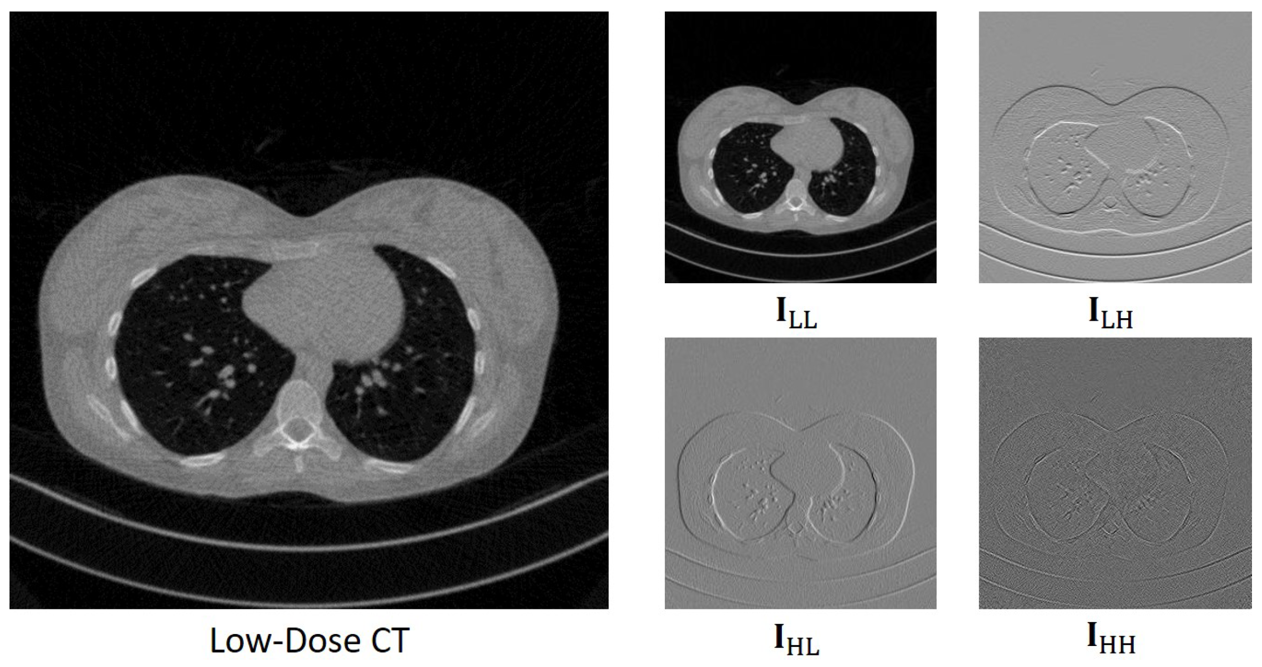
To optimize the performance of the Transformer without the constraints of GPU memory, a viable solution is to use low-resolution images, since it reduces the device resource consumption of the models. The wavelet transform, a prevalent technique in image processing, offers a reversible method to halve image size by decomposing signals into different frequency bands, achieving this without any loss of information and thereby reducing computational resource demands. Another significant advantage of the wavelet transform is the ease of handling sub-band signals separately and effectively. Integrating the wavelet transform with deep learning has already shown impressive results in several studies. Bae et al. [30] demonstrated the effectiveness of learning on wavelet sub-bands, introducing the wavelet residual network for image restoration. Guo et al. [31] developed a deep wavelet super-resolution network to retrieve missing details in wavelet sub-bands between low and high-resolution images. Similarly, Liu et al. [32] proposed the multi-level wavelet-CNN (MWCNN) for image restoration, utilizing multi-level wavelet transform for various tasks and obtaining a PSNR of over 32 dB with a run time of less than 0.1 s. In the context of image denoising, the decomposition of noise along with the image allows for tailored noise suppression methods in different sub-bands. Such an approach is anticipated to surpass traditional noise reduction methods that operate directly in the image domain.
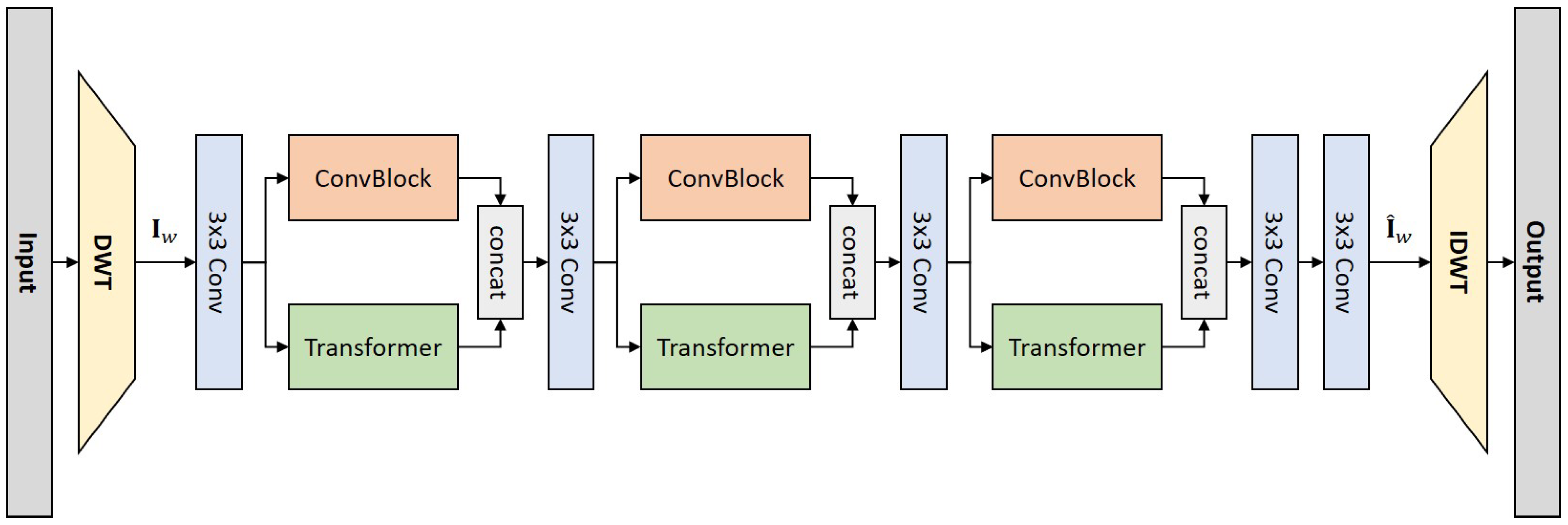
In this work, we leverage the wavelet transform as the sampling framework and attenuate noise in the wavelet domain. Drawing inspiration from previous LDCT denoising research, we introduce a novel denoising network that synergizes the strengths of both CNNs and Transformers. Our approach employs the discrete wavelet transform (DWT) for image downsampling and the inverse discrete wavelet transform (IDWT) for upsampling. The network architecture features dual forward denoising streams, which effectively combine the local feature extraction capability of the convolution operation with the fine-grained information connectivity modelling prowess of Transformers. This integration allows for the extraction of CT image features at various levels. Trained under a specifically designed dual-domain loss function, our proposed network, termed WaveletDFDS-Net, demonstrates enhanced performance in exquisite detail restoration, effectively utilizing the complementary advantages of CNNs and Transformers in the context of LDCT denoising. In summary, this paper introduces the following key contributions to LDCT denoising:
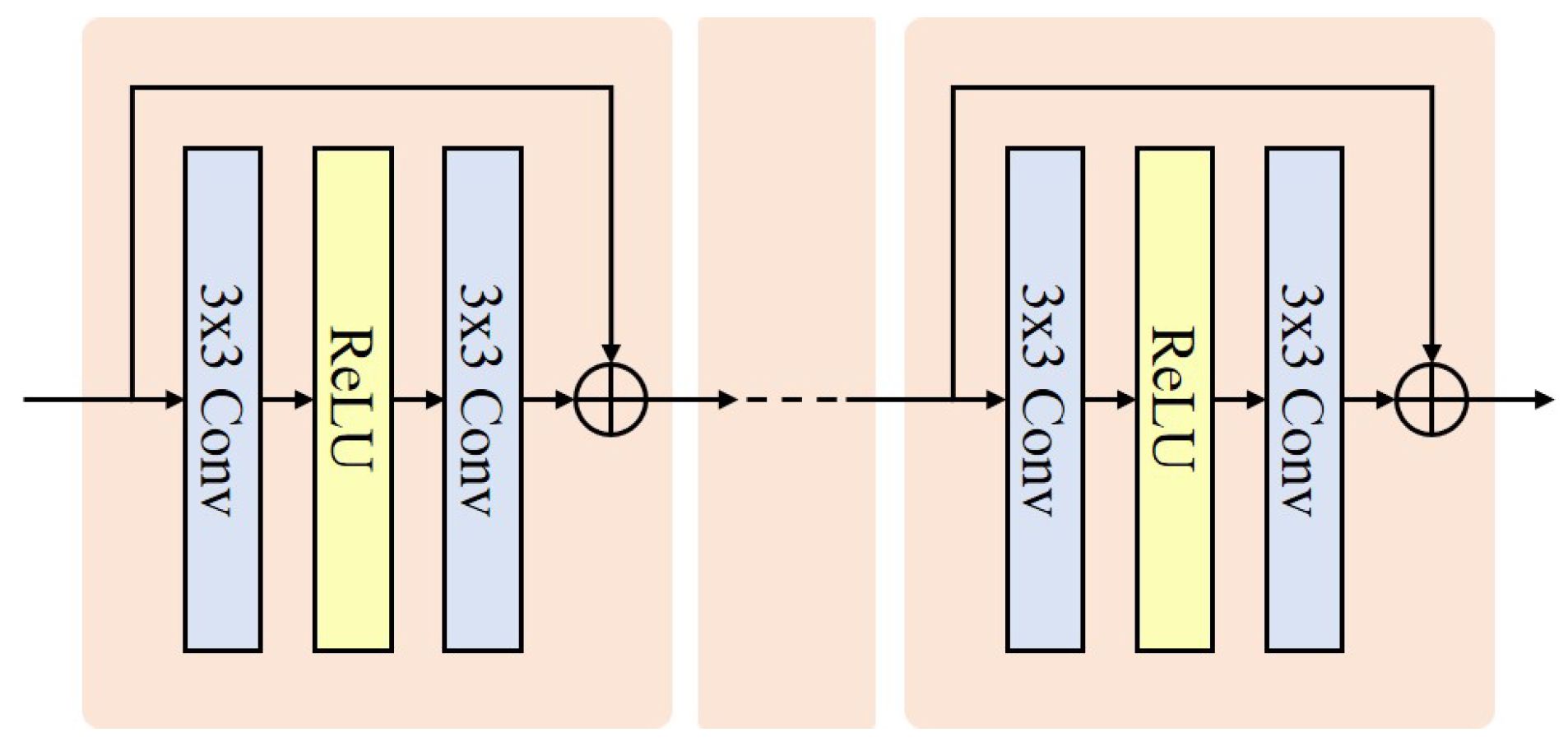
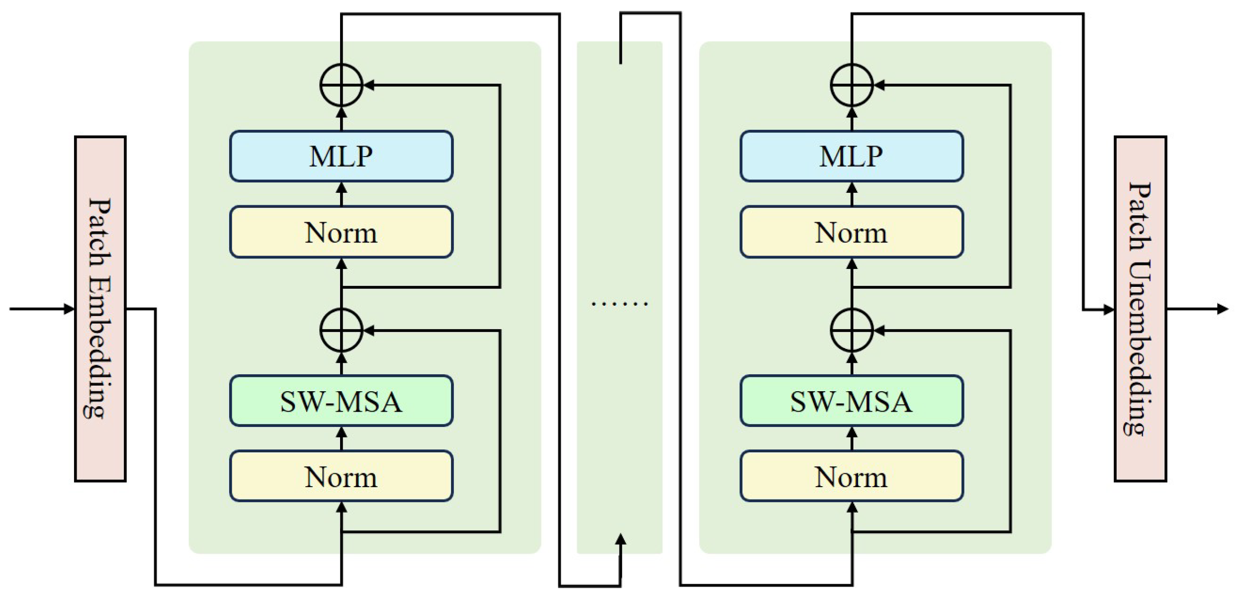
  • Development of WaveletDFDS-Net: We propose WaveletDFDS-Net, which harnesses the local feature extraction capabilities of the convolution operation and the pixel-level information encoding strength of Transformers and reduces noise in the wavelet domain. This network is designed to efficiently extract LDCT image wavelet features from various levels in parallel, leading to more effective noise suppression in LDCT images and fewer computing resource requirements.
  • Dual-domain compound loss function: An efficient dual-domain compound loss function has been formulated to train WaveletDFDS-Net. This function incorporates an additional wavelet domain loss as an auxiliary component to the image domain loss, aiming to achieve high-fidelity detail restoration in the denoising process.
  • Superior experimental outcomes: Our experimental evaluations demonstrate that the proposed method outperforms existing well-known denoising techniques. WaveletDF DS-Net not only shows improved performance metrics but also produces images of higher quality, underlining its effectiveness in LDCT denoising applications.
The remainder of this paper is structured as follows: Section 2 provides a comprehensive description of the proposed WaveletDFDS-Net and the dual-domain compound loss mechanism. Section 3 outlines the experimental setup, presents the outcomes of various ablation studies, and compares experimental results. The paper concludes with Section 5, summarizing the key findings and contributions of this research.

2. Methodology

2.1. Problem Formulation

The noise in LDCT is primarily composed of statistical noise, also known as quantum noise, and electronic noise, which arise during the signal acquisition process [33]. To simplify the complex degradation transition from NDCT to LDCT in the image domain, the noisy LDCT image I ld R H × W can be represented as:
I ld = D ( I nd ) ,
where I nd R H × W denotes the NDCT image, and D : R H × W R H × W symbolizes the degradation process. Consequently, the task is reformulated as finding a denoising function f to minimize the following objective function:
argmin f | | f ( I ld ) I nd | | .
In our approach, the denoising function is characterized by a neural network, denoted as f θ , where θ represents the network parameters. This function is obtained through deep learning training techniques.
In the proposed model, we implement the DWT operation as the downsampling layer to process the input image, transforming the input image I ld into four distinct wavelet sub-images:
I LL , I LH , I HL , I HH = DWT ( I ld ) ,
where I LL , I LH , I HL , I HH R H 2 × W 2 represent sub-images capturing various frequency components. This process effectively separates high- and low-frequency information while reducing the resolution by half. An example of DWT decomposition is depicted in Figure 1, illustrating the different sub-images: I LL represents the low-frequency sub-image, essentially an approximation of the original image; I LH and I HL capture horizontal and vertical edge features, respectively; I HH reflects the diagonal edge feature. The sub-images are then concatenated into a latent feature I ω R H 2 × W 2 × 4 , upon which the designated network operates to diminish noise in the wavelet domain:
I ^ ω = f θ ( I ω ) .
In this equation, I ^ ω R H 2 × W 2 × 4 signifies the denoised latent feature. The final phase of our model utilizes the IDWT operation as an upsampling layer. This step converts the feature back to its original resolution and reconstructs the denoised image I ^ nd R H × W :
I ^ nd = IDWT ( I ^ ω ) .
Consequently, the objective function is finally reformulated as:
argmin θ | | I ^ nd I nd | | .
Given the reversible nature of the DWT, this function can be optimized either in the image domain, the wavelet domain, or a combination of both.

2.2. Network Architecture

As proven by many previous works, the convolution operation has the ability to capture positional information in images, which is lacking in Transformers. Although positional embedding methods have been introduced in Transformers to mitigate this shortfall, they are generally less efficient and more computationally intensive compared to a convolution operation [34,35]. Transformers, on the other hand, excel at encoding pixel-level features from a global sequence, a function that convolution operations struggle with due to their limited receptive fields. Our approach synergises convolution and Transformer operations, harnessing their respective strengths and counterbalancing their weaknesses.
Specifically, the proposed WaveletDFDS-Net, as illustrated in Figure 2, features a distinctive architecture primarily composed of dual forward denoising streams, including a convolution operation branch and a Transformer branch. These streams are intricately designed for efficient feature extraction and aggregation within the wavelet domain. At the network’s inception, a 3 × 3 convolutional layer is utilized to extract the fundamental information as the initial features and elevate the wavelet sub-images to a higher dimensional space. Conversely, towards the end of the network, another 3 × 3 convolutional layer is employed to reduce the dimensionality. This design deviates from conventional methods that predominantly rely on stacking Transformer layers. Instead, the WaveletDFDS-Net innovatively incorporates a CNN branch in parallel to the Transformer layers. Throughout the feature processing phase, information is synergistically integrated between these two branches multiple times. This approach is instrumental in enhancing the learning of the feature representation, ensuring a more robust and efficient noise reduction process.
In our model, the high-dimensional features are processed through dual forward streams. One stream, comprising a ConvBlock with multiple residual blocks, is dedicated to extracting local, coarse features. Concurrently, the other stream, built from several vision Transformer blocks, focuses on modelling pixel relationships and capturing pixel-wise, fine-grained information. The specific structures of the ConvBlock and Transformer are shown in Figure 3 and Figure 4, respectively. This dual-stream structure enables each pathway to specialize in different aspects without mutual interference, mitigating the issue of information dilution often encountered in densely stacked neural networks. The distinct natures of the convolution operation and the Transformer allow for a multi-level information extraction. By merging the outputs from the ConvBlock and the Transformer, a richer feature set is obtained. A subsequent 3 × 3 convolutional layer then adeptly weights and fuses these features, facilitating adaptive redundancy filtering while maintaining dimensional consistency. This enhances the efficiency of subsequent processes. The WaveletDFDS-Net repeats this processing mode thrice, effectively balancing model complexity and performance.

2.3. Loss Function

In this work, two loss functions were employed for denoising LDCT images: the L1 loss and the Structural Similarity Index Measure (SSIM) loss [36]. The SSIM loss, formulated as follows, plays a crucial role in evaluating image quality:
L SSIM ( X , Y ) = 1 N i = 1 N 1 SSIM ( X i , Y i ) ,
SSIM ( X , Y ) = ( 2 μ X μ Y + C 1 ) ( 2 σ XY + C 2 ) ( μ X 2 + μ Y 2 + C 1 ) ( σ X 2 + σ Y 2 + C 2 ) ,
where μ and σ represent the mean and standard deviation of the images, respectively, and σ XY 2 denotes the covariance between X and Y . C 1 and C 2 are constants that stabilize the division with weak denominators. This SSIM loss is particularly effective in maintaining the structural integrity and similarity between the denoised and original images, which is vital in medical imaging applications like LDCT. The integration of L1 loss complements the SSIM by focusing on pixel-wise differences, thus ensuring both global structural fidelity and local accuracy in the denoised images.
To train the proposed model, we initially utilized the L1 loss as the primary loss function, aiming to minimize the L1 distance between the predicted output I ^ nd and the ground truth I nd . However, relying solely on the image domain loss did not fully harness the model’s capabilities. The wavelet transform offered the unique ability to reduce noise in various sub-bands, applying tailored methods based on the specific characteristics of each sub-image. To enhance denoising performance, we formulated a dual-domain compound loss function that integrated the image domain L1 loss with a wavelet-domain detail restoration loss. Given that the low-frequency sub-image I LL retained most of the original image’s features and details, we incorporated an SSIM loss specifically in this sub-band to bolster structure information learning, as SSIM effectively quantifies the structural similarity between two images. The wavelet domain loss thus served as an auxiliary regulatory component relative to the image domain loss.
In summary, the compound loss function was defined as:
L compound = L 1 ( I ^ nd , I nd ) + λ × L SSIM ( I ^ LL , I LL ) .
In this equation, I ^ LL denotes the low-frequency sub-image of predicted output I ^ nd , and I LL corresponds to the low-frequency sub-image of NDCT image I nd . The parameter λ represents the weight of the total wavelet domain loss. In our experiments, we set λ = 0.05.

3. Experiments

3.1. Implementation Details

In this study, we standardized the feature channels across all layers at 64. Each ConvBlock comprised two residual blocks, while the Transformer segment included two Swin Transformer blocks adopted from the Swin Transformer model [26]. Various combinations were explored, with findings detailed in Section 3.4. Both the window size and the number of attention heads within the Transformer were set to eight for convenient operation, and the MLP dimension count quadrupled the number of feature channels used as default in the paper [26].
All our experiments were conducted on a workstation equipped with an Intel(R) i9-9900K CPU, 64 GB RAM and dual NVIDIA GeForce RTX 2080Ti graphics cards, utilizing Pytorch 1.8.1. We trained our model for 100,000 iterations using the Adam optimizer with β 1 = 0.9 , β 2 = 0.99 , with a batch size of four. The initial learning rate was set to 0.001.

3.2. Dataset Description

In this study, we used the publicly accessible dataset, Low-Dose CT Image and Projection Data [37], to evaluate our proposed method. This dataset includes a variety of exam types: 99 head scans, 100 chest scans, and 100 abdomen scans. All these scans were acquired at standard dose levels, and each case was processed to include a second simulated lower-dose projection dataset—head and abdomen scans were provided at 25% of the normal dose, and chest scans at 10%. In our experiments, we randomly selected 2000 slices from 20 patients for each exam type. These images were then normalized to a range of [0, 1], using exam type-specific window settings: [0, 80] HU for head scans, [−1000, 1000] HU for chest scans, and [−300, 300] HU for abdomen scans. Moreover, the large background of all of the head CT images was removed and only the centre 320 × 320 was preserved. Then, all datasets were divided into training, validation, and test sets, where the training sets were used to train the proposed network, the validation sets were used to monitor the networks’ performance during training, and the test sets were used to evaluate the networks after training.

3.3. Evaluation Metrics

To facilitate a thorough comparison, we employed three quantitative metrics, including the SSIM, Peak Signal-to-Noise Ratio (PSNR), and Root-Mean-Square Error (RMSE), for evaluating the image quality of various compared denoising methods. Among the three metrics, SSIM and RMSE primarily gauge pixel-wise similarity, whereas PSNR quantifies the ratio between the maximal potential signal value and the interfering noise, thereby assessing signal representation accuracy. Specifically, the SSIM, as represented by Equation (8), is meant to compare the brightness, contrast, and structure between two images, while the PSNR, usually measured in decibels (dB), is defined as the following function:
PSNR ( X , Y ) = 10 lg M a x V a l u e 2 MSE ( X , Y ) ,
MSE ( X , Y ) = 1 n i = 1 n [ X i Y i ] 2 ,
where M a x V a l u e is the largest possible pixel value, n is the total number of pixels, and MSE calculates the mean squared error of two images. Furthermore, the RMSE is the square root of the MSE, which mainly reflects the average deviation between images:
RMSE ( X , Y ) = MSE ( X , Y ) .
Optimal noise reduction performance is indicated by higher values of SSIM and PSNR, coupled with a lower RMSE.

3.4. Model and Performance Trade-Offs

We firstly conducted several experiments on the chest dataset to evaluate the efficiency of WaveletDFDS-Net with various configurations. Table 1 illustrates that as the number of residual blocks N c per ConvBlock increased, there was a significant rise in the number of network parameters and floating-point operations (FLOPs). Concurrently, the number of Transformer blocks N t per Transformer markedly impacted inference time per image and GPU memory usage. Although an expanded model demonstrated enhanced information learning capability, this did not necessarily translate into a higher PSNR. In certain configurations, the PSNR improvement was minimal and did not justify the increased computational resource consumption. To balance model size and denoising performance, we settled on two residual blocks N c and two Transformer blocks N t for each unit, which remains the standard unless noted otherwise in the following sections.

3.5. Ablation Study

3.5.1. Ablation of Denoising Stream

To verify the effectiveness of the proposed convolution operation and Transformer parallel denoising stream strategy, we performed the ablation experiments on the chest dataset to compare the performance of the proposed network with the settings of only the Transformer stream ( N c = 0 ) and only the convolution stream ( N t = 0 ). Experimental results are shown in Table 2. We observe that denoising only using convolution operation was more time-consuming, while the addition of transformer stream could accelerate the inference to some extent. Moreover, the performance of the network with only a single denoising branch was similar, which was significantly lower than that of the network with two branches, although this combination increased requirements in terms of the number of network parameters, GPU memory, and FLOPs. Apparently, these results fully validated the necessity and effectiveness of the combination of convolution operation and Transformer, since this combination allowed the network to extract features from different levels and remove noise to a greater extent.

3.5.2. Ablation of DWT

To test the denoising performance of WaveletDFDS-Net in the image domain and wavelet domain, we conducted comparative experiments on the chest dataset. As shown in Table 3, it is obvious that the proposed network trained in the image domain took up more computing resources. Except the number of network parameters, the use of the wavelet transform dramatically reduced the execution time, GPU memory consumption, and FLOPs of the network while improving the SSIM, PSNR, and RMSE. Therefore, the power of the wavelet transform was that it not only significantly reduced the consumption of computing resources by efficiently halving the image resolution but also helped to detect noise in different frequency bands and obtain a better denoising effect.

3.5.3. Ablation of Loss Function

To prove the effect of the proposed dual-domain compound loss function, we compared the performance of the proposed network trained under three types of loss functions, including the L1 loss, image-domain compound loss, and dual-domain compound loss. As shown in Table 4, the L1 loss was the main component of the three loss functions, all of which were calculated in the image domain. Incorporating the SSIM loss either in the image or wavelet domain enhanced all metrics. However, compared with the image domain SSIM loss that evenly learned the information of different frequency bands, the wavelet-domain SSIM loss, which guided the network to heavily focus on the low-frequency band with more noise components, improved metrics more. Consequently, for optimal denoising performance, the dual-domain compound loss function emerged as the preferred optimization objective for subsequent experiments.

3.6. Experimental Results

Comparison methods: We compared our method with several well-known low-dose CT denoising methods, including BM3D [38] and K-SVD [39], which are the most popular image-based denoising methods, RED-CNN [16], MAP-NN [40], QAE [41], and EDCNN [42], which are CNN-based methods, and TransCT [21] and CTformer [29], which are Transformer-based methods. The training parameters of these competing methods were set according to the recommendations of the original papers.
Here, we firstly tested the execution speed of these comparison methods other than BM3D and K-SVD (non-deep-learning-based methods executing on CPU). Table 5 shows the average inference time of 200 images with a resolution of 512 × 512. We observe that TransCT and CTformer were the fastest and slowest models, with average inference times of 0.0094 s and 0.3624 s per image, respectively. In addition, the proposed network was in the middle among these methods, with lower inference times than those of RED-CNN and CTformer but higher than those of MAP-NN, QAE, EDCNN, and TransCT, with approximately 0.1564 s per image processed. To sum up, even though WaveletDFDS-Net applied the DWT, its model efficiency still lagged behind that of some approaches.
Noise reduction performance: The left section of Table 6 presents the experimental results on the head CT dataset. We observe that the proposed method was superior to all compared methods, with the SSIM and PSNR achieving the highest value and the RMSE the lowest. Figure 5 visualizes the noise reduction effects across different models on this dataset. Notably, BM3D and K-SVD, unlike other compared methods which successfully reduced noise, were less effective in noise reduction, resulting in images still marred by significant noise. In contrast, images denoised by TransCT and CTformer exhibited only slight noise. RED-CNN and EDCNN, while effective in noise reduction, tended to over-smooth the boundaries of distinct soft tissues, thus diminishing clinical diagnostic value. Other comparative methods like MAP-NN and QAE showed similar denoising performance. However, WaveletDFDS-Net stood out for its superior restoration of details, offering a higher quality and fidelity. As shown in Figure 6, the zoomed images over a region of interest have clearer contrasts in the details. The evaluation metrics for the images presented in Figure 5 are detailed in the left section of Table 7.
The middle section of Table 6 displays the experimental results on the chest CT dataset. Analysis of the metric values revealed that WaveletDFDS-Net achieved superior evaluation metrics, surpassing all other models. Figure 7 depicts the image restoration results of the various methods on that dataset. BM3D primarily smoothed the noise, leaving noticeable traces in the denoised images. K-SVD and CTformer exhibited limited noise reduction capabilities, with their outputs retaining significant noise residues in the whole tissue. Some other methods like RED-CNN, EDCNN, and TransCT showed similar denoising effects with higher SSIM and PSNR and lower RMSE than BM3D, K-SVD, and CTformer but tended to produce blurry images. MAP-NN and QAE demonstrated improved denoising performance and image quality. Nevertheless, WaveletDFDS-Net further enhanced the denoising efficiency and restored images with quality closest to NDCT images. Figure 8 enlarges the partial details of the region marked by the red box in Figure 7, which provides a better observation. The quantitative results corresponding to these observations are presented in the middle section of Table 7, related to Figure 7.
The right section of Table 6 presents the experimental results conducted on the abdomen CT dataset, where our proposed model demonstrated superior performance. Figure 9 offers a qualitative comparison of noise reduction in abdomen CT images. K-SVD showed the least effective noise reduction, with its outputs retaining significant noise distributed throughout the organs. Similar to findings in the head and chest datasets, images denoised by BM3D, TransCT, and CTformer exhibited minor noise spots. In addition, other compared methods, while displaying lower noise levels and better evaluation metrics, still faced the issue of blurriness. In contrast, the proposed model trained with the compound loss not only attained higher metric values but also minimized image error, thereby restoring clear feature details. All these fine details could be more obviously observed in the zoomed images of Figure 10. The evaluation metrics for the images in Figure 9 are detailed in the right section of Table 7.
Table 7. Quantitative results of different denoising methods for Figure 5, Figure 7, and Figure 9.
MethodsFigure 5Figure 7Figure 9
SSIMPSNRRMSESSIMPSNRRMSESSIMPSNRRMSE
Before Denoising0.874723.99640.06310.749632.82460.02280.871930.17380.0310
BM3D [38]0.885325.14560.05530.926038.45590.01190.915333.65690.0208
K-SVD [39]0.875124.73580.05800.813534.82530.01810.890631.61050.0263
RED-CNN [16]0.897328.33960.03830.943139.39660.01070.921734.60280.0186
MAP-NN [40]0.900228.30030.03850.947739.66700.01040.923334.58020.0187
QAE [41]0.899828.35020.03820.945739.51150.01060.922234.59990.0186
EDCNN [42]0.899428.26220.03860.944839.49220.01060.922734.45350.0189
TransCT [21]0.861726.66720.04640.942839.12290.01110.911033.54110.0210
CTformer [29]0.891828.02420.03970.919038.03470.01250.904333.80390.0204
WaveletDFDS-Net (Ours)0.901828.35400.03820.954340.17040.00980.924634.65190.0185

4. Discussion

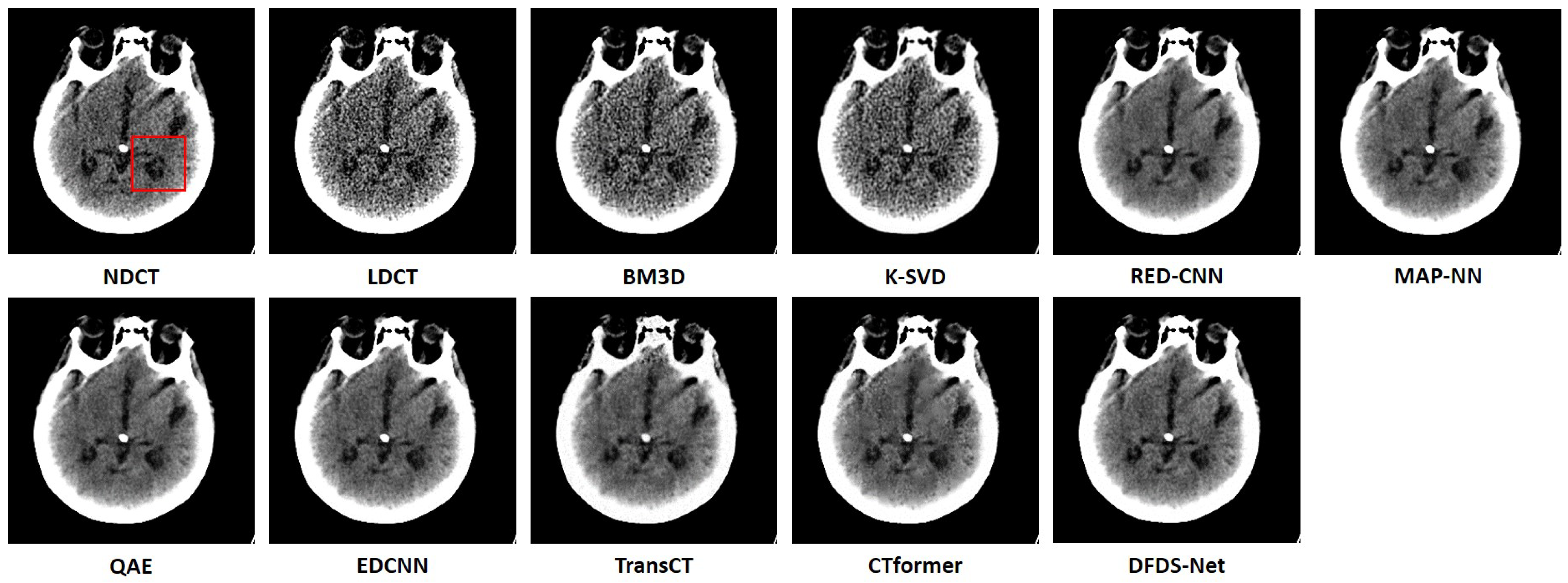
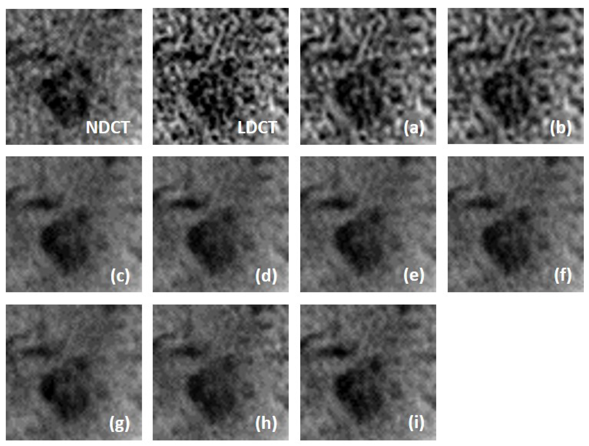
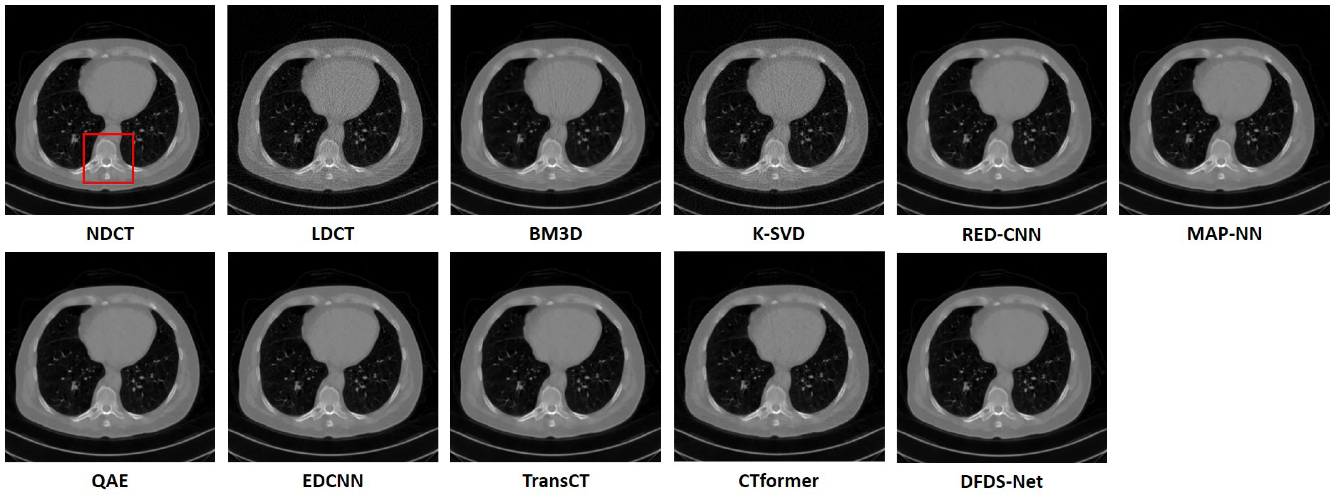
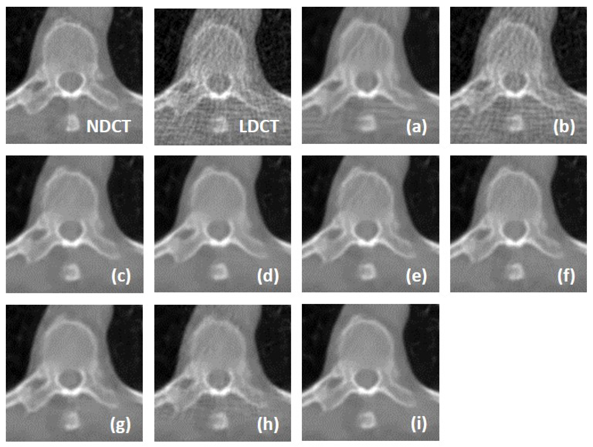
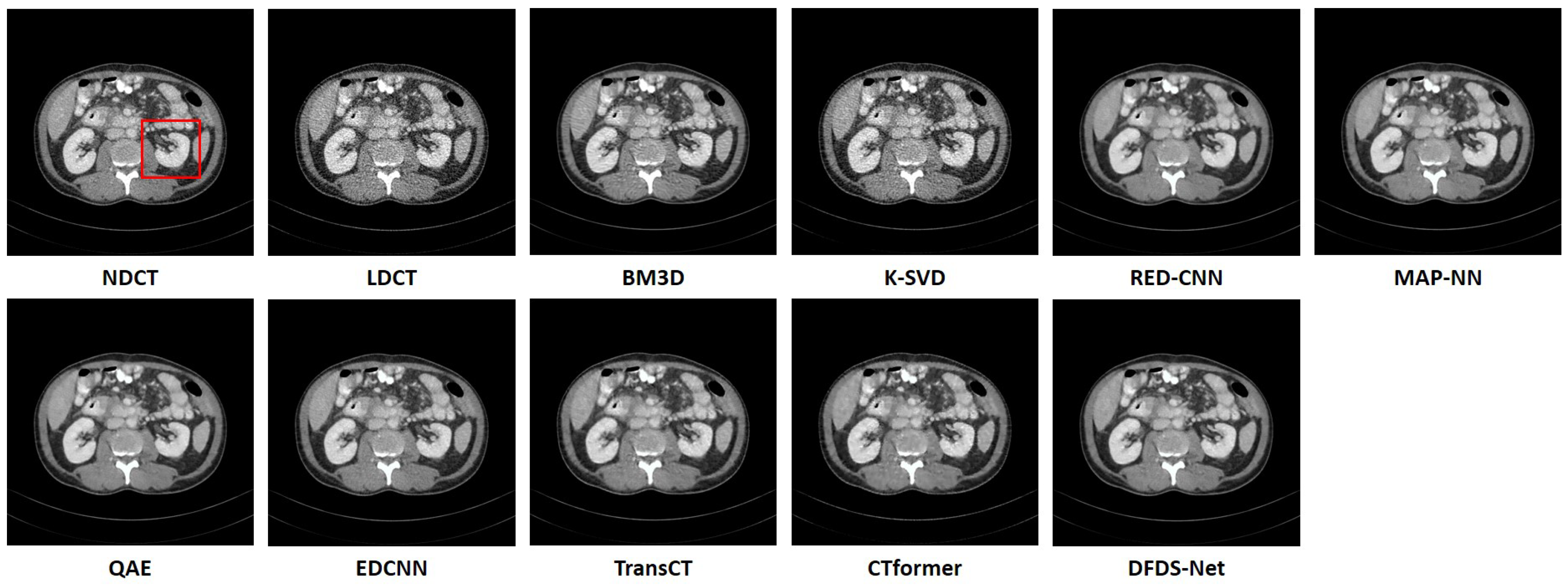
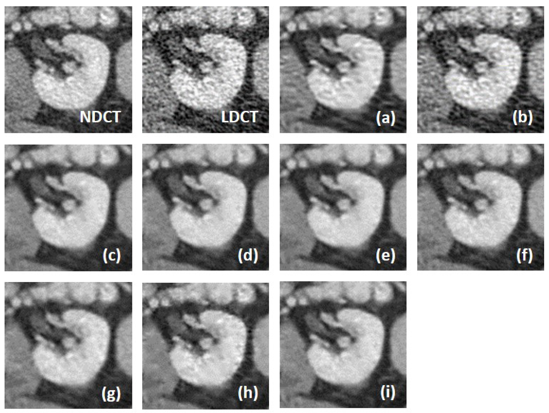
We fully compared the efficiency and performance of WaveletDFDS-Net with several well-known LDCT denoising methods and quantitatively and visually presented the experimental results in the above sections. As one of the classical image-denoising algorithms, BM3D groups patches by searching for similar regions in the image and performs collaborative filtering by the group to reduce noise. Although excellent achievements on natural image tasks have been obtained, the drawbacks are also obvious. For images with uneven noise distribution or pixels entangled with noise, BM3D has a limited denoising effect, whose results always suffer from noise residue or blurring. Similarly, classically, K-SVD is a dictionary learning method that applies an SVD decomposition of images and selects the term with the minimum error as the updated dictionary parameter to iteratively optimize until the noise level converges. However, in our case, since the noise of LDCT was introduced in the projection domain and converted into a more complex distribution in the image domain, the capacity of the SVD decomposition was insufficient, resulting in a minimum noise reduction effect of K-SVD in our experiments.
Different from the above two methods, the deep learning strategy had a more powerful denoising ability. RED-CNN, as an early model, constructs an encoder–decoder structure with residual connections that demonstrated far better performance than K-SVD and BM3D through end-to-end training, as shown in the experimental results in Table 6. MAP-NN adaptively performs progressive noise reduction by looping through a convolutional network and takes a discriminator as one of the supervisors to train its network. These improvements contribute to increased evaluation metrics. Based on Red-CNN, QAE employs quadratic neurons (executing a quadratic operation on the input data) instead of the original inner product for high-order nonlinear sparse representation with a reasonable model complexity. As the efficiency shown in Table 5 and performance shown in Table 6, QAE comprehensively outperformed RED-CNN. EDCNN focuses on the extraction of image edge information and introduces an edge enhancement module in the first layer of the dense connection network to improve the effect of image edge restoration. Our experiments confirmed that EDCNN restored clearer boundaries of distinct organs than other models. However, all of these methods were inferior to WaveletDFDS-Net in denoising performance due to the inherent receptive field limitations of convolution.
TransCT and CTformer are two kinds of Transformer-based LDCT noise reduction models; the former separates the high-frequency content and low-frequency content of LDCT images and then mainly denoises the high-frequency part, while the latter designs a token-to-token learning strategy that encompasses local contextual information via token rearrangement rather than convolution operation. Although neither requires much computing resources, the performance is not satisfactory. Obviously, even though Transformer has the long-range feature extraction capabilities that CNN lacks, it does not reach its potential if it is used incorrectly. In contrast to these comparison methods, WaveletDFDS-Net builds two parallel branches based on Transformer and convolution operations, respectively, to learn the noise distribution at the fine-gained level and local coarse level on multiple wavelet bands to improve noise reduction performance in a cooperative manner. WaveletDFDS-Net shows promising potential to avoid the misrepresentation of anatomical structures in images and ultimately lead to better patient outcomes through more accurate diagnoses and treatments.
While the proposed methods demonstrate superior denoising capabilities, some aspects could be improved. Firstly, the concurrent architecture of CNNs and Transformers does not fully exploit the synergistic potential between these technologies, resulting in modest improvements in efficiency and experimental metrics. Secondly, the training of WaveletDFDS-Net relies on a supervised learning strategy requiring a substantial dataset of paired LDCT and NDCT images, which are challenging to acquire in real-world clinical settings, thus restricting practical applicability.

5. Conclusions

In this paper, we introduced WaveletDFDS-Net, a dual forward denoising stream network for low-dose CT noise reduction. This network synergized the local feature extraction prowess of the convolution operation and the exquisite information connectivity capabilities of Transformers to extract multi-level image features, enhancing the learning of feature representation, resulting in more robust and efficient denoising performance. Moreover, WaveletDFDS-Net employed the wavelet transform as the sampling unit to reduce the image size without any information loss, and then processed image features in the wavelet domain. Furthermore, we also devised a unique dual-domain loss function to enhance detail restoration. Experimental results across three different types of CT datasets demonstrated that our method outperformed the compared baseline models in both evaluation metrics and visual quality. Future work will focus on developing an unsupervised version of WaveletDFDS-Net to mitigate the dependency on paired training datasets and broaden its applicability in clinical environments.

Author Contributions

Conceptualization, Y.Z. and Z.K.; methodology, Y.Z. and Z.K.; validation, Y.Z.; formal analysis, Y.Z.; investigation, Y.Z.; resources, Z.K. and T.H.; writing—original draft preparation, Y.Z.; writing—review and editing, T.H., E.A., H.L. and L.D.; visualization, Y.Z.; supervision, Z.K. and T.H.; project administration, Z.K.; funding acquisition, Z.K. and T.H. All authors have read and agreed to the published version of the manuscript.

Funding

The work of Zhengmin Kong was supported in part by the grant from Nation Key R&D Program of China (2021ZD0112702), National Natural Science Foundation of China (No. 62173256). The work of Tao Huang was supported in part by the Australian Government through the Australian Research Council’s Discovery Projects Funding Scheme under Project DP220101634. The work of Li Ding was supported in part by the grant from National Natural Science Foundation of China (No. 62373290).

Data Availability Statement

Publicly accessible dataset: https://www.cancerimagingarchive.net/collection/ldct-and-projection-data/#citations (accessed on 5 August 2023).

Conflicts of Interest

The authors declare that they have no known competing financial interests or personal relationships which could have appeared to influence the work reported in this paper.

References

  1. Einstein, A.J.; Henzlova, M.J.; Rajagopalan, S. Estimating risk of cancer associated with radiation exposure from 64-slice computed tomography coronary angiography. JAMA 2007, 298, 317–323. [Google Scholar] [CrossRef]
  2. Smith-Bindman, R.; Lipson, J.; Marcus, R.; Kim, K.P.; Mahesh, M.; Gould, R.; De González, A.B.; Miglioretti, D.L. Radiation dose associated with common computed tomography examinations and the associated lifetime attributable risk of cancer. Arch. Intern. Med. 2009, 169, 2078–2086. [Google Scholar] [CrossRef]
  3. Brenner, D.J.; Hall, E.J. Computed tomography—An increasing source of radiation exposure. N. Engl. J. Med. 2007, 357, 2277–2284. [Google Scholar] [CrossRef]
  4. Naidich, D.P.; Marshall, C.H.; Gribbin, C.; Arams, R.S.; McCauley, D.I. Low-dose CT of the lungs: Preliminary observations. Radiology 1990, 175, 729–731. [Google Scholar] [CrossRef] [PubMed]
  5. Wang, J.; Li, T.; Lu, H.; Liang, Z. Penalized weighted least-squares approach to sinogram noise reduction and image reconstruction for low-dose X-ray computed tomography. IEEE Trans. Med. Imaging 2006, 25, 1272–1283. [Google Scholar] [CrossRef] [PubMed]
  6. Manduca, A.; Yu, L.; Trzasko, J.D.; Khaylova, N.; Kofler, J.M.; McCollough, C.M.; Fletcher, J.G. Projection space denoising with bilateral filtering and CT noise modeling for dose reduction in CT. Med. Phys. 2009, 36, 4911–4919. [Google Scholar] [CrossRef] [PubMed]
  7. Wang, J.; Lu, H.; Li, T.; Liang, Z. Sinogram noise reduction for low-dose CT by statistics-based nonlinear filters. In Proceedings of the Medical Imaging 2005: Image Processing, San Diego, CA, USA, 12–17 February 2005; SPIE: Bellingham, WA, USA, 2005; Volume 5747, pp. 2058–2066. [Google Scholar]
  8. Hara, A.K.; Paden, R.G.; Silva, A.C.; Kujak, J.L.; Lawder, H.J.; Pavlicek, W. Iterative reconstruction technique for reducing body radiation dose at CT: Feasibility study. Am. J. Roentgenol. 2009, 193, 764–771. [Google Scholar] [CrossRef]
  9. Beister, M.; Kolditz, D.; Kalender, W.A. Iterative reconstruction methods in X-ray CT. Phys. Medica 2012, 28, 94–108. [Google Scholar] [CrossRef]
  10. Geyer, L.L.; Schoepf, U.J.; Meinel, F.G.; Nance, J.W., Jr.; Bastarrika, G.; Leipsic, J.A.; Paul, N.S.; Rengo, M.; Laghi, A.; De Cecco, C.N. State of the art: Iterative CT reconstruction techniques. Radiology 2015, 276, 339–357. [Google Scholar] [CrossRef]
  11. Ma, J.; Huang, J.; Feng, Q.; Zhang, H.; Lu, H.; Liang, Z.; Chen, W. Low-dose computed tomography image restoration using previous normal-dose scan. Med. Phys. 2011, 38, 5713–5731. [Google Scholar] [CrossRef]
  12. Li, Z.; Yu, L.; Trzasko, J.D.; Lake, D.S.; Blezek, D.J.; Fletcher, J.G.; McCollough, C.H.; Manduca, A. Adaptive nonlocal means filtering based on local noise level for CT denoising. Med. Phys. 2014, 41, 011908. [Google Scholar] [CrossRef] [PubMed]
  13. Kang, D.; Slomka, P.; Nakazato, R.; Woo, J.; Berman, D.S.; Kuo, C.C.J.; Dey, D. Image denoising of low-radiation dose coronary CT angiography by an adaptive block-matching 3D algorithm. In Proceedings of the Medical Imaging 2013: Image Processing, Lake Buena Vista, FL, USA, 10–12 February 2013; SPIE: Bellingham, WA, USA, 2013; Volume 8669, pp. 671–676. [Google Scholar]
  14. Chen, H.; Zhang, Y.; Zhang, W.; Liao, P.; Li, K.; Zhou, J.; Wang, G. Low-dose CT via convolutional neural network. Biomed. Opt. Express 2017, 8, 679–694. [Google Scholar] [CrossRef] [PubMed]
  15. Gondara, L. Medical image denoising using convolutional denoising autoencoders. In Proceedings of the 2016 IEEE 16th International Conference on Data Mining Workshops (ICDMW), Barcelona, Spain, 12–15 December 2016; IEEE: Piscataway, NJ, USA, 2016; pp. 241–246. [Google Scholar]
  16. Chen, H.; Zhang, Y.; Kalra, M.K.; Lin, F.; Chen, Y.; Liao, P.; Zhou, J.; Wang, G. Low-dose CT with a residual encoder-decoder convolutional neural network. IEEE Trans. Med. Imaging 2017, 36, 2524–2535. [Google Scholar] [CrossRef] [PubMed]
  17. Yang, Q.; Yan, P.; Zhang, Y.; Yu, H.; Shi, Y.; Mou, X.; Kalra, M.K.; Zhang, Y.; Sun, L.; Wang, G. Low-dose CT image denoising using a generative adversarial network with Wasserstein distance and perceptual loss. IEEE Trans. Med. Imaging 2018, 37, 1348–1357. [Google Scholar] [CrossRef] [PubMed]
  18. Kang, E.; Koo, H.J.; Yang, D.H.; Seo, J.B.; Ye, J.C. Cycle-consistent adversarial denoising network for multiphase coronary CT angiography. Med. Phys. 2019, 46, 550–562. [Google Scholar] [CrossRef] [PubMed]
  19. Lee, K.; Jeong, W.K. ISCL: Interdependent self-cooperative learning for unpaired image denoising. IEEE Trans. Med. Imaging 2021, 40, 3238–3248. [Google Scholar] [CrossRef] [PubMed]
  20. Zhu, J.Y.; Park, T.; Isola, P.; Efros, A.A. Unpaired image-to-image translation using cycle-consistent adversarial networks. In Proceedings of the IEEE International Conference on Computer Vision, Venice, Italy, 22–29 October 2017; pp. 2223–2232. [Google Scholar]
  21. Zhang, Z.; Yu, L.; Liang, X.; Zhao, W.; Xing, L. TransCT: Dual-path transformer for low dose computed tomography. In Proceedings of the Medical Image Computing and Computer Assisted Intervention–MICCAI 2021: 24th International Conference, Strasbourg, France, 27 September–1 October 2021; Proceedings, Part VI 24. Springer: Berlin/Heidelberg, Germany, 2021; pp. 55–64. [Google Scholar]
  22. Dosovitskiy, A.; Beyer, L.; Kolesnikov, A.; Weissenborn, D.; Zhai, X.; Unterthiner, T.; Dehghani, M.; Minderer, M.; Heigold, G.; Gelly, S.; et al. An image is worth 16 × 16 words: Transformers for image recognition at scale. arXiv 2020, arXiv:2010.11929. [Google Scholar]
  23. Yang, F.; Yang, H.; Fu, J.; Lu, H.; Guo, B. Learning texture transformer network for image super-resolution. In Proceedings of the IEEE/CVF Conference on Computer Vision and Pattern Recognition, Seattle, WA, USA, 13–19 June 2020; pp. 5791–5800. [Google Scholar]
  24. Chen, H.; Wang, Y.; Guo, T.; Xu, C.; Deng, Y.; Liu, Z.; Ma, S.; Xu, C.; Xu, C.; Gao, W. Pre-trained image processing transformer. In Proceedings of the IEEE/CVF Conference on Computer Vision and Pattern Recognition, Nashville, TN, USA, 20–25 June 2021; pp. 12299–12310. [Google Scholar]
  25. Liang, J.; Cao, J.; Sun, G.; Zhang, K.; Van Gool, L.; Timofte, R. Swinir: Image restoration using swin transformer. In Proceedings of the IEEE/CVF International Conference on Computer Vision, Montreal, BC, Canada, 11–17 October 2021; pp. 1833–1844. [Google Scholar]
  26. Liu, Z.; Lin, Y.; Cao, Y.; Hu, H.; Wei, Y.; Zhang, Z.; Lin, S.; Guo, B. Swin transformer: Hierarchical vision transformer using shifted windows. In Proceedings of the IEEE/CVF International Conference on Computer Vision (ICCV), Montreal, BC, Canada, 11–17 October 2021; pp. 10012–10022. [Google Scholar]
  27. Wang, Z.; Cun, X.; Bao, J.; Zhou, W.; Liu, J.; Li, H. Uformer: A general u-shaped transformer for image restoration. In Proceedings of the IEEE/CVF Conference on Computer Vision and Pattern Recognition, New Orleans, LA, USA, 18–24 June 2022; pp. 17683–17693. [Google Scholar]
  28. Luthra, A.; Sulakhe, H.; Mittal, T.; Iyer, A.; Yadav, S. Eformer: Edge enhancement based transformer for medical image denoising. arXiv 2021, arXiv:2109.08044. [Google Scholar] [CrossRef]
  29. Wang, D.; Fan, F.; Wu, Z.; Liu, R.; Wang, F.; Yu, H. CTformer: Convolution-free Token2Token dilated vision transformer for low-dose CT denoising. Phys. Med. Biol. 2023, 68, 065012. [Google Scholar] [CrossRef] [PubMed]
  30. Bae, W.; Yoo, J.; Chul Ye, J. Beyond deep residual learning for image restoration: Persistent homology-guided manifold simplification. In Proceedings of the IEEE Conference on Computer Vision and Pattern Recognition Workshops, Honolulu, HI, USA, 21–26 July 2017; pp. 145–153. [Google Scholar]
  31. Guo, T.; Seyed Mousavi, H.; Huu Vu, T.; Monga, V. Deep wavelet prediction for image super-resolution. In Proceedings of the IEEE Conference on Computer Vision and Pattern Recognition Workshops, Honolulu, HI, USA, 21–26 July 2017; pp. 104–113. [Google Scholar]
  32. Liu, P.; Zhang, H.; Zhang, K.; Lin, L.; Zuo, W. Multi-level wavelet-CNN for image restoration. In Proceedings of the IEEE Conference on Computer Vision and Pattern Recognition Workshops, Salt Lake City, UT, USA, 18–22 June 2018; pp. 773–782. [Google Scholar]
  33. Diwakar, M.; Kumar, M. A review on CT image noise and its denoising. Biomed. Signal Process. Control 2018, 42, 73–88. [Google Scholar] [CrossRef]
  34. Islam, M.A.; Jia, S.; Bruce, N.D. How much position information do convolutional neural networks encode? arXiv 2020, arXiv:2001.08248. [Google Scholar] [CrossRef]
  35. Guo, J.; Han, K.; Wu, H.; Tang, Y.; Chen, X.; Wang, Y.; Xu, C. Cmt: Convolutional neural networks meet vision transformers. In Proceedings of the IEEE/CVF Conference on Computer Vision and Pattern Recognition, New Orleans, LA, USA, 18–24 June 2022; pp. 12175–12185. [Google Scholar]
  36. Wang, Z.; Bovik, A.C.; Sheikh, H.R.; Simoncelli, E.P. Image quality assessment: From error visibility to structural similarity. IEEE Trans. Image Process. 2004, 13, 600–612. [Google Scholar] [CrossRef] [PubMed]
  37. McCollough, C.; Chen, B.; Holmes, D.; Duan, X.; Yu, Z.; Xu, L.; Leng, S.; Fletcher, J. Low dose CT image and projection data [data set]. Cancer Imaging Arch. 2020, 10. [Google Scholar] [CrossRef]
  38. Dabov, K.; Foi, A.; Katkovnik, V.; Egiazarian, K. Image denoising by sparse 3-D transform-domain collaborative filtering. IEEE Trans. Image Process. 2007, 16, 2080–2095. [Google Scholar] [CrossRef] [PubMed]
  39. Chen, Y.; Yin, X.; Shi, L.; Shu, H.; Luo, L.; Coatrieux, J.L.; Toumoulin, C. Improving abdomen tumor low-dose CT images using a fast dictionary learning based processing. Phys. Med. Biol. 2013, 58, 5803. [Google Scholar] [CrossRef] [PubMed]
  40. Shan, H.; Padole, A.; Homayounieh, F.; Kruger, U.; Khera, R.D.; Nitiwarangkul, C.; Kalra, M.K.; Wang, G. Competitive performance of a modularized deep neural network compared to commercial algorithms for low-dose CT image reconstruction. Nat. Mach. Intell. 2019, 1, 269–276. [Google Scholar] [CrossRef]
  41. Fan, F.; Shan, H.; Kalra, M.K.; Singh, R.; Qian, G.; Getzin, M.; Teng, Y.; Hahn, J.; Wang, G. Quadratic autoencoder (Q-AE) for low-dose CT denoising. IEEE Trans. Med. Imaging 2019, 39, 2035–2050. [Google Scholar] [CrossRef]
  42. Liang, T.; Jin, Y.; Li, Y.; Wang, T. Edcnn: Edge enhancement-based densely connected network with compound loss for low-dose ct denoising. In Proceedings of the 2020 15th IEEE International Conference on Signal Processing (ICSP), Beijing, China, 6–9 December 2020; IEEE: Piscataway, NJ, USA, 2020; Volume 1, pp. 193–198. [Google Scholar]
Figure 1. An example of wavelet transform. Left is the original low-dose CT image, and right is the sub-images after the DWT operation, where L and H refer to the low- and high-pass filter, respectively. The display window is [−1000, 1000] HU.
Electronics 13 01906 g001
Figure 2. The structure of WaveletDFDS-Net. It uses the discrete wavelet transform (DWT) and inverse discrete wavelet transform (IDWT) as the sampling units and contains two denoising streams, namely, a convolution stream constructed by a convolutional block (ConvBlock) and a Transformer stream constructed by Transformer, and integrates latent feature by concatenating (concat) two branches during the feature processing procedure.
Electronics 13 01906 g002
Figure 3. ConvBlock structure, which consists of several residual blocks.
Electronics 13 01906 g003
Figure 4. Transformer structure. The basic block is adopted from the Swin Transformer.
Electronics 13 01906 g004
Figure 5. Comparison of the qualitative performance of WaveletDFDS-Net and other well-known low-dose CT denoising methods on the head dataset. The display window is [0, 80] HU.
Electronics 13 01906 g005
Figure 6. The zoomed images over the region of interest (ROI) marked by the red box in Figure 5. (a) BM3D, (b) K-SVD, (c) RED-CNN, (d) MAP-NN, (e) QAE, (f) EDCNN, (g) TransCT, (h) CTformer, (i) WaveletDFDS-Net.
Electronics 13 01906 g006
Figure 7. Comparison of the qualitative performance of WaveletDFDS-Net and other well-known low-dose CT denoising methods on the chest dataset. The display window is [−1000, 1000] HU.
Electronics 13 01906 g007
Figure 8. The zoomed images over the region of interest (ROI) marked by the red box in Figure 7. (a) BM3D, (b) K-SVD, (c) RED-CNN, (d) MAP-NN, (e) QAE, (f) EDCNN, (g) TransCT, (h) CTformer, (i) WaveletDFDS-Net.
Electronics 13 01906 g008
Figure 9. Comparison of the qualitative performance of WaveletDFDS-Net and other well-known low-dose CT denoising methods on the abdomen dataset. The display window is [−160, 240] HU.
Electronics 13 01906 g009
Figure 10. The zoomed images over the region of interest (ROI) marked by the red box in Figure 9. (a) BM3D, (b) K-SVD, (c) RED-CNN, (d) MAP-NN, (e) QAE, (f) EDCNN, (g) TransCT, (h) CTformer, (i) WaveletDFDS-Net.
Electronics 13 01906 g010
Table 1. Comparison of model size and performance among different combinations.
N c N t ParamsTimeGPUFLOPsSSIMPSNRRMSE
110.60 M0.08 s930 MB29.40 G0.921537.90930.0133
120.75 M0.15 s1555 MB29.45 G0.921337.93630.0133
141.05 M0.31 s2805 MB29.55 G0.916437.69800.0137
220.97 M0.16 s1699 MB43.98 G0.922438.02510.0132
241.27 M0.31 s2949 MB44.08 G0.919637.82880.0135
N c and N t refer to the number of residual blocks per ConvBlock and the number of Transformer blocks per Transformer, respectively. Model size is evaluated by the number of network parameters (Params), GPU memory usage (GPU), and floating point operations (FLOPs), while performance is reflected by the model inference time per image (Time) and three types of evaluation metrics.
Table 2. Performance comparison between different denoising strategies.
Denoising StreamParamsTimeGPUFLOPsSSIMPSNRRMSE
Transformer-only0.42 M0.15 s1411 MB7.67 G0.920037.67790.0137
Conv-only0.56 M0.20 s353 MB36.63 G0.9198037.63080.0138
Both0.97 M0.16 s1699 MB43.98 G0.922438.02510.0132
Table 3. Performance comparison of WaveletDFDS-Net with or without the DWT.
DWTParamsTimeGPUFLOPsSSIMPSNRRMSE
0.97 M1.88 s6787 MB175.02 G0.921237.72220.0136
0.97 M0.16 s1699 MB43.98 G0.922438.02510.0132
Table 4. Performance comparison of WaveletDFDS-Net trained with different loss functions.
Loss TypeSSIMPSNRRMSE
L1 (image)0.922438.02510.0132
L1 (image) + L SIMM (image)0.925538.08330.0131
L1 (image) + L SIMM (wavelet)0.926938.13430.0130
Table 5. Comparison of inference time between different methods.
MethodTime
BM3D-
K-SVD-
RED-CNN0.2412 s
MAP-NN0.0615 s
QAE0.0210 s
EDCNN0.0161 s
TransCT0.0094 s
CTformer0.3624 s
WaveletDFDS-Net (Ours)0.1564 s
Table 6. Quantitative comparison with well-known low-dose CT denoising methods on the head, chest, and abdomen datasets.
MethodsHead (25% Dose)Chest (10% Dose)Abdomen (25% Dose)
SSIMPSNRRMSESSIMPSNRRMSESSIMPSNRRMSE
Before Denoising0.860523.56360.06820.624429.41610.03820.748924.92970.0649
BM3D [38]0.870624.62190.06060.831534.46760.02280.796727.61560.0504
K-SVD [39]0.858924.16190.06310.706531.60840.02950.781126.87500.0518
RED-CNN [16]0.884528.03800.04060.912637.16350.01460.822830.28980.0337
MAP-NN [40]0.887728.00460.04070.919137.60040.01380.826530.25100.0338
QAE [41]0.887428.06600.04040.918637.57800.01390.825630.31970.0336
EDCNN [42]0.887027.95330.04090.914837.47870.01400.826130.19520.0340
TransCT [21]0.845326.35170.04930.911236.97570.01490.799529.42160.0375
CTformer [29]0.875827.68400.04220.864135.46480.01790.800529.49020.0368
WaveletDFDS-Net (Ours)0.889028.07180.04030.926938.13430.01300.829730.36800.0334
Disclaimer/Publisher’s Note: The statements, opinions and data contained in all publications are solely those of the individual author(s) and contributor(s) and not of MDPI and/or the editor(s). MDPI and/or the editor(s) disclaim responsibility for any injury to people or property resulting from any ideas, methods, instructions or products referred to in the content.

