Abstract
Developments in digital twins are driven by the availability of sensor technologies, big data, first principles knowledge, and advanced analytics. In this paper, we discuss these changes at a conceptual level, presenting a shift from nominal engineering, aiming at design optimisation, to performance engineering, aiming at adaptable monitoring diagnostic, prognostic, and prescriptive capabilities. A key element introduced here is the role of emulators in this transformation. Emulators, also called surrogate models or metamodels, provide monitoring and diagnostic capabilities. In particular, we focus on an optimisation goal combining optimised and robust performance derived from stochastic emulators. We demonstrate the methodology using two open-source examples and show how emulators can be used to complement finite element and computational fluid dynamic models in digital twin frameworks. The case studies consist of a mechanical system and a biological production process.
1. Introduction
A heightened level of maturity in the management of systems and processes is achieved by combining physical assets with digital assets in order to deliver enhanced analytic capabilities. This integrated layer is usually labelled a digital twin [1,2,3,4,5]. We emphasise the role of emulators in digital twining strategies, which are focused on the operational phase of systems and processes. This paper covers topics such as hybrid models, soft sensors, digital twins, emulators, computational fluid dynamics, and finite element methods. Digital twins are used for optimisation, monitoring, diagnostics, prognostics, and prescriptive analytic capabilities. Computational models, such as finite element methods (FEM) and computational fluid dynamics (CFD), are used by engineers to study properties of products and systems [1,2,3,6]. Such numerical models are used in troubleshooting and forensic fault analysis. In this paper, we focus on the role of emulators in digital twin applications. In particular, we focus on an optimisation goal combining optimised and robust performance derived from stochastic emulators. We also distinguish between emulators used in monitoring and emulators used in optimisation and diagnostics. These applications provide adequate performance of digital twins in terms of speed and accuracy and an analytic layer enabling the transformation from engineering of design to engineering of performance. We refer to two examples: a piston used in a combustion engine and PENSIM, a simulator of penicillin fermentation production. The piston models the operation of a piston with seven input factors and one response variable, which is the cycle time. The piston simulator is implemented in R, Python, JMP, and Matlab; see [7,8,9]. The PENSIM simulation software is used to model penicillin production in a fed-batch fermentor [10,11]. It is used operationally to monitor and process troubleshooting activities. These case studies involve electronics in their controllers and fault diagnostics. Here, we take a wide-angle perspective and model their overall performance. Digital twins complement or substitute physical experiments with software-based simulation experiments [11,12,13]. They also enable the application of soft sensors derived computationally from laboratory data and sensors located on systems and processors. Computer experiments, or simulations, are typically analysed with Gaussian Process Models [8,13,14,15,16,17]. In the text section, we also introduce multifidelity and Bayesian hierarchical models [18,19]. Such models permit the building of knowledge of physical systems and support decision-making for the design and monitoring of such systems. A digital twin can be used to run experiments by a number of runs of a simulation code where factors are parametrised as a subset of the code’s inputs. The contributions of this paper include (a) a description of emulators derived from computationally intensive models using Gaussian processes, (b) consideration of hybrid models combining physical and simulations-based data, (c) applications of emulators for enhanced monitoring and diagnostics, (d) incorporation of emulators in digital twin platforms, (e) an introduction of stochastic emulators to optimise performance and robustness, and (f) case studies demonstrating the above. Section 2 discusses how emulators are designed and analysed. Section 3 and Section 4 include case studies of simulators and their emulators. The last section includes a discussion and conclusions.
2. Methodology: The Design and Analysis of Emulators
2.1. Design of Emulators of Systems
A typical computer experiment or simulation requires efficient strategies for sampling the input space, deriving accurate predictions in untried inputs, and providing an easy-to-interpret description of knowledge. If randomness is present in the input variables, the sources of uncertainty are difficult to split. To illustrate [20], we will consider three types of errors: simulation-model error, metamodel error, and implementation error; we will then suggest mathematical programming models. The behaviour of a physical system can be represented by f, such that:
where x = (x1, x2, …, xp) ∈ is the input variable, y ∈ R is the output variable, and is the input variable space and a subset of Rp. The deterministic function f does not need to have an analytic representation. Frequently, the solution of such systems of equations is an approximation of model (1), g, where:
y = f(x1, x2, …, xp)
y = g(x1, x2, …, xp)
The model g(∙) needs to be close enough to the real one (f). An approximate model (g) is referred to as an emulator. The use of models in engineering design practice is extensive, and metamodel (2) is required to approximate model (1) as accurately as possible.
2.2. Computer Experiments from Simulations
The common designs in computer experiments are designs based on the selection of the points in the experimental region (11). Two approaches are implemented: stochastic and deterministic. The uncertainty in the stochastic process used for modelling computer experiments represents a lack of knowledge of the exact relationship between input variables and response, a gap referred to as model bias in experimental design [21,22,23,24,25]. We want to determine experimental points Dn = {x1, x2, …, xn} that ensure the deviation between model (1) and metamodel (2):
is as small as possible. The experimental region of a computer experiment can be defined as the unit cube Cp (0 ≤ xj ≤ 1, j = 1, 2, …, p), where p is the number of the variables. Emulators or surrogate models are used to minimise (3). An example is the Kriging model that assumes that the experimental responses are realisations of zero-mean Gaussian random field plus a regression term:
where x ∈ D ⊂ Rp, is a set of specified trend functions and is a set of coefficients. Z(x) is a Gaussian random process with zero mean and stationary covariance over D so that and , where is the process variance, and R is a correlation function depending on the displacement vector h between any pair of points in D and on a parameter θ. A typical correlation function is:
Specifically, one often applies the power exponential family:
where θ = (θ1,θ2,…,θp,s)T, θj are positive scale parameters, and s is a common smoothing parameter. Parameter θj describes how rapidly correlation decays in direction j with increasing distance hj. The positive correlation between outputs in (6) diminishes with increasing distance between input locations. If θj = θ ∀j, the correlation depends only on the distance |h| between any pair of points (x and x + h). Parameter s describes the pattern of the correlation decay. When s = 2, the correlation function is Gaussian. The power exponential family: s = 2 gives infinitely differentiable trajectories for the Gaussian process realisations. Values s < 2 correspond to non-differentiable trajectories. The prediction of the response at a new point x0 is based on prior information in a set of experimental points , with xi∈D for I = 1, 2, …, n. A common prediction criterion is the mean squared prediction error. Under the hypothesis that the joint random variable is a multivariate normal, denoted as , with , the conditional mean of Y(x) at the new point x0, given the process data, , is:
where f0 is the m × 1 vector of the trend functions in x0; F is the n × m matrix of the trend functions computed in ; r0 is the correlation vector ; and R is the n × n correlation matrix whose (i,j) element is .
The predictor is the best linear unbiased predictor of Y(x0) because it minimizes the mean squared prediction error, , and is also unique. For more information on computer experiments, see [8,13,14].
2.3. Optimising Products and Processes
In optimising systems and processes, we aim to be on target with minimum variability. A comprehensive approach to designing and analysing computer experiments for system process optimisation is the stochastic emulator [8]. A stochastic emulator is a model of the variability in the data derived by running computer experiments on the data model. It combines optimisation of a model of performance and variability to ensure, as best as possible, both on-target performance and minimal variability. The key steps of setting up a stochastic emulator are as follows:
- Modelling: This can be derived from the results of an initial experiment, purely on theoretical grounds, or by a combination of the two.
- Uncertainty: Characterising uncertainty in the system is describing how the input factors vary.
- Computer experiment design: Plan a computer experimental design of the input factors.
- Generate simulated data: Apply the noise distributions in the computer experimental design.
- Stochastic emulator: Construct a model that relates response variables to the design factor settings.
- Optimisation: Determine a setup that ensures optimisation of both target performance and robustness.
The stochastic emulator has online capabilities that can be incorporated into digital twins that handle unexpected operational conditions. The digital twin provides monitoring capabilities that compare healthy system-predicted behaviour to the actual behaviour and flag out-of-control behaviour. To provide diagnostic capabilities, we developed an emulator to identify variable importance and a prediction profiler. Based on this capability, we can classify system behaviour patterns and identify input values that affect system behaviour patterns. In this context, the response, Y, corresponds to a tracking sensor, such as a vibration sensor, and input variables, X, such as factors affecting the system’s operational profile. To develop prognostic capabilities, we developed a model with the response YF corresponding to a degradation variable or faults. The stochastic emulator provides prescriptive and optimisation capabilities.
2.4. Other Methods
Hybrid models combining physical and computer experiments are gaining attention [2]. In this section, we briefly review multi-fidelity and hierarchical Bayes models that integrate information derived from various types of experiments.
In multi-fidelity models, we combine data from various sources differing in levels of detail and sophistication [18]. The basic model is
where is the fidelity level of the experimental system, is the systematic error, and is the random error ( corresponds to the real system). There are also primary terms and potential terms; only the primary terms, , are included in the regression model.
The experimental planning model in the context of variable fidelity experimentation involves selecting the number of runs, the location, and the fidelity level associated with each point by minimising the expected integrated mean squared error subject to cost constraints [26].
The recursive Bayesian hierarchical model [19] permits the combination of information from expert opinion, computer experiments, and physical experiments in a unified regression model. It is based on updating the initial beliefs of experts by incorporating computer simulation and physical experiment data.
Both the recursive Bayesian hierarchical integrated model, combining expert opinion with simulation and physical experiments, and the variable fidelity level experiments have proven useful in practical applications where experiments are conducted in different conditions and prior experience has been accumulated.
We mention these methods for completeness and refer to the cited literature for more details. In the next two sections, we provide examples of how computer experiments and stochastic emulators can be used to provide enhanced capabilities for monitoring, diagnostic, prognostic, and optimisation of systems and processes. The piston simulator will be used to demonstrate the fitting of a Gaussian process emulator, and PENSIM will take us further and show how to optimise a process with a stochastic emulator.
3. Case Study 1: The Piston Simulator
This simulator response variable is measured by the cycle time of a full revolution in seconds. The seven factors that possibly affect cycle time are (1) M—piston weight, (2) S—piston surface area, (3) V0—initial gas volume, (4) K—spring coefficient, (5) P0—atmospheric pressure, (6) T—ambient temperature, and (7) T0—gas temperature. The levels of these factors represent extremes in the operating range.
The simulator is running at given factor level combinations with uncertainty in the factors. The piston simulator is available in R and JMP in Python and in Matlab [7,8,9].
As a first step, we show on the left of Figure 1 a control chart of the piston running at the nominal level of all seven factors. For more information on control charts, see [8]. The left of Figure 1 represents normal operating conditions. The control chart tracks 30 samples of five consecutive cycle times—a total of 150 observations. The bottom chart tracks standard deviations of five consecutive cycle times representing local uncertainty in system performance. Overall, the piston runs under stable conditions, i.e., within control limits. On the right of Figure 1, we see the next 30 samples of size 5, with the earlier control limits shown on the left chart. A dramatic reduction in cycle time is observed. What causes such a drop?
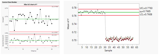
Figure 1.
Control charts of cycle time (left) for 30 and another 30 (right) consecutive observations (JMP 17.0).
To better understand the behaviour of the piston and provide diagnostic information, we run a space-filling Latin hypercube design consisting of 150 experimental runs. For more information on such space-filling designs, see [8,12]. Figure 2 shows the experimental array with two-way scatterplots.
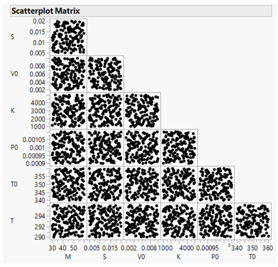
Figure 2.
Space-filling design of the piston simulator; seven factors (JMP 17.0).
For these experiments, we fit a Gaussian process. Figure 3 shows the process parameters, and Figure 4 shows the profiler and the marginal effects of the seven factors on the piston cycle time. We can see that changes in V0 and K have an effect on cycle time. Figure 3 indicates the total sensitivity for V0 and K to be 0.49 and 0.30, respectively. This confirms that K and V0 have high leverage on cycle time. This emulator model can now be used to investigate what-if scenarios and help troubleshoot investigations. Incorporating such a model in a digital twin of an operating piston provides enhanced monitoring and diagnostic capabilities. For more information on the properties of the piston simulator, see [7,8].
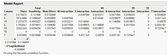
Figure 3.
Gaussian process fit for the piton simulator space-filling experiments. (JMP 17.0).

Figure 4.
Profiler for the piton simulator space-filling experiments. (JMP 17.0).
4. Case Study 2: The PENSIM Simulator
The PENSIM simulation models penicillin production [10,11,27,28]. It includes variables such as pH, temperature, aeration rate, agitation power, feed flow rate of the substrate, and a Raman probe. The simulated process outputs we use here are (1) P: final penicillin concentration and (2) X: final biomass concentration. Our goal is to maximise P, with a lower specification limit of 0.8 g/L, and minimise X, with an upper specification of 12 g/L. In Figure 5, we show the distributions of P and X over the operational design space. The production process in this space resulted in 20% of batches being defective on P (below 0.8) and 5% of batches being defective on X (above 12).
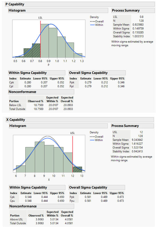
Figure 5.
Distribution of the responses P and X over the full design space (JMP 17.0).
To run the simulation, we set up the following process variables: 1. S0: initial sugar concentration, 2. X0: initial biomass concentration, 3. pH: pH set point, 4. T: temperature set point, 5. air: aeration set up, 6. agitation: agitation rate, 7. time: culture time, and 8. feed: sugar feed rate. The variables that vary during production are Fg: aeration rate, RPM: agitation rate, Fs: substrate feed, Ts: substrate temperature, S: substrate, DO: dissolved oxygen, Uvis: viscosity, CO2: off-gas CO2, Hi: heat inflow, Ti: temperature inflow, Ho: heat outflow, and Fw: water for injection. We run, with the PENSIM simulator, a space-filling computer experiment with 128 runs constrained in the hypercube (see Table 1).

Table 1.
Factors and factor levels used in space-filling experiments.
With these experiments, we fit a Gaussian process model to P and X and derive Figure 6.
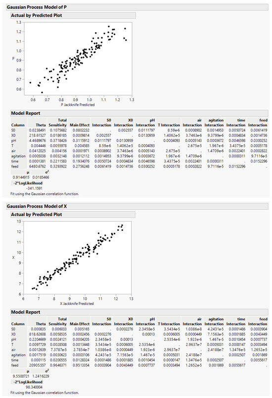
Figure 6.
Gaussian process fit responses P and X over the full design space (JMP 17.0).
If we set up the eight factors at their midpoint values and run simulations for normal distributions of the process variable, we obtain for P a defect rate of 5.7%, with a mean of 0.95 g/L and standard deviation of 0.096, and for X, we obtain a defect rate of 0.64%, with a mean of 9.3 g/L and a standard deviation of 1.04. If we run the stochastic emulator and optimise the defect rate, we obtain an optimal P setup, as displayed in Table 2.

Table 2.
Factor level combinations of optimal setup.
This yields for P a defect rate of 0%, with a mean of 1.26 and a standard deviation of 0.076, and, for X, a defect rate of 9.7%, with a mean of 11.16 and a standard deviation of 0.748.
P and X are jointly increasing so that their targets of maximisation and minimisation collide. Figure 7 shows their scatterplots for different classes of pH. Feed is indicated by colour of the points, from blue (0.0225) up to red (0.045). A pH above 4.4 with feed below 0.04 results in P and X within specifications.
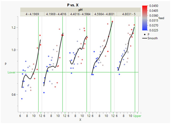
Figure 7.
P versus X scatterplots in various pH categories. The colour of points indicates the level of feed (JMP 17.0).
Increasing feed increases X with little effect on pH. P, however, is affected by both feed and pH and their interaction. To increase P, both must increase, as shown in Figure 8. We can optimise both pH and P, for example, using desirability functions or Pareto front optimisation.
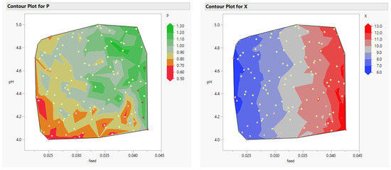
Figure 8.
Contour plots of pH versus feed, for P (left) and X (right), with observations used to fit the Gaussian model marked as dots (JMP 17.0).
Both the piston simulator and PENSIM are simulators based on engineering knowledge. We showed, with the piston simulator, how an emulator can be used to monitor an operating system. This requires a model fed by sensor data that computes a response variable. Comparing a computed response with an observed response provides for effective monitoring. We can, therefore, conduct statistical process control on expected response and on the delta between actual and expected response. Once an out-of-control signal is triggered, the emulator will direct us to possible causes. In the piston case, V0 and K are the first variables to be considered. The PENSIM simulator was used here to demonstrate an application of a stochastic emulator that optimises a process for both performance and robustness. Another analytic capability not demonstrated here is prognostic. This is achieved by implementing time series forecasting models and analysing degradation reliability.
5. Discussion and Conclusions
Digital twins have been initially conceptualised in [4]. The evolution of meaning and applications following that has varied across domains and functionality. An attempt to describe a taxonomy of digital twins is provided in [5].
In this study, we apply emulators incorporating uncertainty in engineering models in order to achieve enhanced performance through extended monitoring, diagnostic, prognostic, and prescriptive capabilities. The digital twin we consider is a container of digital assets where data are stored and analysed in line with [29]. We focus on the application of stochastic emulators as an element in digital twins. Mechanistic-based finite element methods (FEM) and computational fluid dynamic (CFD) approaches have been proposed over three decades ago and, through emulators, can now be incorporated in digital twins. The availability of sensor technologies is creating a need and opportunity for integrating operational data through such models. This has also been incorporated in stochastic FEM [30]. Another approach in a Bayesian framework is statistical FEM [31]. Both stochastic FEM and statistical FEM were designed as offline methods aiming at the system and process design stage. Applying them in online digital systems requires adaptations, such as the emulator Gaussian process method presented here. Examples of such applications are provided in [6,29]. A wide-angle view of state-of-the-art theory and practice, challenges, and open research questions for digital twins is provided in [32].
The objective of this paper is to address some of the analytic challenges facing modern systems and processes where new levels of performance and quality can be achieved with modern sensor technologies.
The specific contributions of this paper include:
- A description of emulators that can be derived from computationally intensive models using Gaussian processes.
- Consideration of hybrid models combining physical and simulations-based data.
- Applications of emulators for enhanced monitoring and diagnostics.
- Incorporation of emulators in digital twin platforms.
- An introduction of stochastic emulators to optimise performance and robustness.
- Case studies demonstrating the above.
A general scope perspective considers a shift from design engineering to performance engineering. Digital twins and emulators support such a transition.
Funding
This research received no external funding.
Data Availability Statement
Data derived from public domain resource.
Conflicts of Interest
The author declares no conflict of interest.
References
- Kenett, R.S.; Bortman, J. The digital twin in Industry 4.0: A wide-angle perspective. Qual. Reliab. Eng. Int. 2022, 38, 1357–1366. [Google Scholar] [CrossRef]
- Chinesta, F.; Cueto, E.; Abisset-Chavanne, E.; Duval, J.L.; El Khaldi, F. Virtual, Digital and Hybrid Twins: A New Paradigm in Data-Based Engineering and Engineered Data. Arch. Comput. Methods Eng. 2018, 27, 105–134. [Google Scholar] [CrossRef]
- Gabriel, D.; Bortman, J.; Kenett, R.S. Development of an Operational Digital Twin of a Locomotive Parking Brake for Fault Diagnosis. Sci. Rep. 2023, 13, 17959. [Google Scholar]
- Grieves, M. Digital twin: Manufacturing excellence through virtual factory replication. White Pap. 2014, 1, 1–7. [Google Scholar]
- Van der Valk, H.; Haße, H.; Möller, F.; Arbter, M.; Henning, J.L.; Otto, B. A Taxonomy of Digital Twins. In Proceedings of the AMCIS, Virtual, 10–14 August 2020. [Google Scholar]
- Zienkiewicz, O.C. The Finite Element Methods in Engineering Science; McGraw-Hill: New York, NY, USA, 1971. [Google Scholar]
- Kenett, R.S.; Zacks, S.; Gedeck, P. Modern Statistics: A Computer-Based Approach with Python; Birkhäuser: Basel, Switzerland, 2022. [Google Scholar]
- Kenett, R.S.; Zacks, S.; Gedeck, P. Industrial Statistics: A Computer-Based Approach with Python; Springer Nature: New York, NY, USA, 2023. [Google Scholar]
- Simon Fraser Virtual Lab. Available online: https://www.sfu.ca/~ssurjano/emulat.html (accessed on 20 May 2023).
- Birol, I.; Undey, C.; Birol, G.; Cinar, A. A web-based simulator for penicillin fermentation. Int. J. Eng. Simul. 2001, 2, 24–30. [Google Scholar]
- Birol, G.; Ündey, C.; Çinar, A. A modular simulation package for fed-batch fermentation: Penicillin production. Comput. Chem. Eng. 2002, 26, 1553–1565. [Google Scholar] [CrossRef]
- Santner, T.J.; Williams, B.J.; Notz, W.I.; Williams, B.J. The Design and Analysis of Computer Experiments; Springer: New York, NY, USA, 2003; Volume 1. [Google Scholar]
- Kenett, R.S.; Vicario, G. Challenges and opportunities in simulations and computer experiments in industrial statistics: An industry 4.0 perspective. Adv. Theory Simul. 2021, 4, 2000254. [Google Scholar] [CrossRef]
- Vakayil, A.; Joseph, V.R. A Global-Local Approximation Framework for Large-Scale Gaussian Process Modeling. Technometrics 2024, 66, 295–305. [Google Scholar] [CrossRef]
- Sack, J.; Welch, W.J.; Mitchell, T.J.; Wynn, H.P. Design and analysis of computer experiments (with discussion). Stat. Sci. 1989, 4, 409–423. [Google Scholar]
- Roustant, O.; Joucla, J.; Probst, P. Kriging as an alternative for a more precise analysis of output parameters in nuclear safety—Large break LOCA calculation. Appl. Stoch. Models Bus. Ind. 2010, 26, 565–576. [Google Scholar] [CrossRef]
- Stein, M.L. Interpolation of Spatial Data: Some Theory for Kriging; Springer Science & Business Media: New York, NY, USA, 2012. [Google Scholar]
- Huang, D.; Allen, T.T. Design and analysis of variable fidelity experimentation applied to engine valve heat treatment process design. J. R. Stat. Soc. Ser. C Appl. Stat. 2005, 54, 443–463. [Google Scholar] [CrossRef]
- Reese, C.S.; Wilson, A.G.; Hamada, M.; Martz, H.F.; Ryan, K.J. Integrated analysis of computer and physical experiments. Technometrics 2004, 46, 153–164. [Google Scholar] [CrossRef]
- Stinstra, E.; Hertog, D.D. Robust optimization using computer experiments. Eur. J. Oper. Res. 2008, 191, 816–837. [Google Scholar] [CrossRef]
- Krige, D.G. A statistical approach to some basic mine valuation problems on the Witwatersrand. J. South. Afr. Inst. Min. Metall. 1951, 52, 119–139. [Google Scholar]
- Zhang, Q.; Qiao, P.; Wu, Y. A novel kriging-improved high-dimensional model representation metamodelling technique for approximating high-dimensional problems. Eng. Optim. 2024, 1–24. [Google Scholar] [CrossRef]
- Jones, D.R.; Schonlau, M.; Welch, W.J. Efficient global optimization of expensive black-box functions. J. Glob. Optim. 1998, 13, 455–492. [Google Scholar] [CrossRef]
- Allen, T.T.; Bernshteyn, M.A.; Kabiri-Bamoradian, K. Constructing meta-models for computer experiments. Qual. Control. Appl. Stat. 2004, 49, 321–322. [Google Scholar] [CrossRef]
- Stinstra, E.; Hertog, D.D.; Stehouwer, P.; Vestjens, A. Constrained maximin designs for computer experiments. Technometrics 2003, 45, 340–346. [Google Scholar] [CrossRef]
- Kennedy, M.C.; O’Hagan, A. Predicting the output from a complex computer code when fast approximations are available. Biometrika 2000, 87, 1–13. [Google Scholar] [CrossRef]
- Ahmad, A.; Samad, N.A.F.A.; Wei, C.A. Mathematical Modelling and Analysis of Dynamic Behaviour of a Fed-batch Penicillin G Fermentation Process. In Proceedings of the International Conference on Chemical and Bioprocess Engineering, Kota Kinabalu, Sabah, 27–29 August 2003; Volume 2, pp. 387–394. [Google Scholar]
- PENSIM v2. Available online: http://www.industrialpenicillinsimulation.com/ (accessed on 20 May 2023).
- Stark, R.; Fresemann, C.; Lindow, K. Development and operation of Digital Twins for technical systems and services. CIRP Ann. 2019, 68, 129–132. [Google Scholar] [CrossRef]
- Burczyński, T.; Skrzypczyk, J. Theoretical and computational aspects of the stochastic boundary element method. Comput. Methods Appl. Mech. Eng. 1999, 168, 321–344. [Google Scholar] [CrossRef]
- Girolami, M.; Febrianto, E.; Yin, G.; Cirak, F. The statistical finite element method (statFEM) for coherent synthesis of observation data and model predictions. Comput. Methods Appl. Mech. Eng. 2021, 375, 113533. [Google Scholar] [CrossRef]
- Sharma, A.; Kosasih, E.; Zhang, J.; Brintrup, A.; Calinescu, A. Digital twins: State of the art theory and practice, challenges, and open research questions. J. Ind. Inf. Integr. 2022, 30, 100383. [Google Scholar] [CrossRef]
Disclaimer/Publisher’s Note: The statements, opinions and data contained in all publications are solely those of the individual author(s) and contributor(s) and not of MDPI and/or the editor(s). MDPI and/or the editor(s) disclaim responsibility for any injury to people or property resulting from any ideas, methods, instructions or products referred to in the content. |
© 2024 by the author. Licensee MDPI, Basel, Switzerland. This article is an open access article distributed under the terms and conditions of the Creative Commons Attribution (CC BY) license (https://creativecommons.org/licenses/by/4.0/).