Article

Comparison of Energy Storage Management Techniques for a Grid-Connected PV- and Battery-Supplied Residential System

Institute of Control and Industrial Electronics, Warsaw University of Technology, 00-662 Warsaw, Poland
*
Author to whom correspondence should be addressed.
Electronics 2024, 13(1), 87; https://doi.org/10.3390/electronics13010087
Submission received: 22 November 2023 / Revised: 19 December 2023 / Accepted: 22 December 2023 / Published: 24 December 2023

Abstract

:
The use of renewable energy sources (RES) such as wind and solar power is increasing rapidly to meet growing electricity demand. However, the intermittent nature of RES poses a challenge to grid stability. Energy storage (ES) technologies offer a solution by adding flexibility to the system. With the emergence of distributed energy resources (DERs) and the transition to prosumer-based electricity systems, energy management systems (EMSs) have become crucial to coordinate the operation of different devices and optimize system efficiency and functionality. This paper presents an EMS for a residential photovoltaic (PV) and battery system that addresses two different functionalities: energy cost minimization, and self-consumption maximization. The proposed EMS takes into account the operational requirements of the devices and their lower-level controllers. A genetic algorithm (GA) is used to solve the optimization problems, ensuring a desired State of Charge (SOC) at the end of the day based on the next day forecast, without discretizing the SOC transitions allowing a continuous search space. The importance of adhering to the manufacturer’s operating specification to avoid premature battery degradation is highlighted, and a comparative analysis is performed with a simple tariff-driven solution, evaluating total cost, energy exchange, and peak power. Tests are carried out in a detailed model, where Power Electronics Converters (PECs) and their local controllers are considered together with the EMS.

1. Introduction

The addition of global renewable electricity capacity of up to 305 GW is expected for the following four years; among the distributed energy resources (DERs), Wind-powered installations and photovoltaic (PV) systems are extensively deployed due to their competitiveness in power generation costs [1]. Despite their advantages, renewable energy sources (RESs) suffer from natural intermittency, and Energy Storage (ES) technologies can help to overcome this drawback by adding flexibility to the system and even providing support functions such as peak-shaving, power reserve, or frequency stabilization of the grid, while maintaining the State of Charge (SOC) within limits [2].
At the residential level, there is an increasing availability of RESs like PV modules, and ES technologies such as lithium-ion batteries, essential to transitioning consumers into prosumers. In this sense, more flexibility is added to the system, with the possibility to provide continuous supply to the local loads in the event of faults or outages. Moreover, the electricity market policies allow to obtain economic benefits for such systems. Therefore, small participants are expected to take part in the upcoming transactive energy market to negotiate between themselves and the Distribution System Operator (DSO) [3]. Even at the residential level, the system becomes more complex and demands coordination between the different devices to harness its full potential effectively. Each system element demands its own needs; in the case of the DERs, the objective is to extract the maximum available power. On the other hand, ES devices must be operated within safe limits to maximize their lifetime without limiting their utilization.
The complicated nature of interactions between consumers, loads, DERs, and the grid creates a need for energy management systems (EMSs) as an indispensable tool to perform real-time monitoring of energy generation and consumption, optimizing energy flow, and guaranteeing the load supply such that the overall residential system operates at the desired operating conditions within the given constraints, and achieves specific goals such as cost reduction [4].
Extensive research has been conducted for the EMS at the residential level, giving special attention to the optimization methods [5,6,7,8,9]. In terms of the solving method, the mixed integer linear programming (MILP) approach is widely adopted. However, several others have been explored, such as dynamic programming (DP), model predictive control (MPC), nonlinear programming (NLP), heuristic methods, like particle swarm optimization (PSO) and genetic algorithms (GA), and the most recent solutions exploit the use of artificial intelligence (AI) techniques including reinforcement learning [10]. However, AI-based solutions face limitations in handling hard constraints that must never be breached in a real environment and transferring learning from simulation-trained models to their implementation in real environments [11].
In [5], a modified PSO is proposed, a dynamic penalty factor is added to the cost function, which has to be tuned and the algorithm is executed each hour without leveraging the information of load and generation profiles from forecast services. An analytical approach to maximize self-consumption is proposed in [6], the initial investment and maintenance expenses are included, and the computational complexity is reduced, but this proposal is only applicable to two-level tariff scenarios. In [7], a modified state-space DP technique is used to achieve a given value of SOC at the end of the day. This method requires the discretization of the SOC, resulting in a discontinuous search space [12]. The DP algorithm has also been implemented in [13] to solve the optimal battery scheduling, considering the battery aging. In this case, the performance of the system is assessed in terms of the net present cost instead of the revenue obtained by the user
A quadratic programming (QP) based scheduling algorithm is used in [14] where different metering topologies, and the sensitivity to battery size are studied. Furthermore, voltage swings due to increased power flow are penalized to reduce the burden on the grid. An improved implementation of the sparrow search algorithm (SSA), together with multiobjective SSA, has been proposed in [15] to solve the energy management problem in the context of source-load-storage aggregation groups connected to a distribution network. For instance, to reduce the stress on the grid and minimize indirect costs such as network expenses, energy exchange minimization has been investigated [8,9]. Despite the objective of energy minimization, economic improvements are also obtained compared to a simple strategy where the battery is only charged when generation is greater than the load demand. Another proposal that addresses energy minimization and battery usage simultaneously, is presented in [16]. The optimization problem is solved with linear programming, and the weighted sum approach is used to integrate the multi-objective cost function into a single objective one. However, results demonstrate to be sensitive to the selection of the weights.
One of the most recent solutions is based on Reinforcement Learning-Techniques. An energy management system based on Proximal Policy Optimization is developed in [17], without requiring forecast services. However, a constant price and feed-in tariff are considered, and extensive training examples and parameter tuning are needed. In contrast to the proposals that deal with large-scale systems, where distributed algorithms are utilized [18], in the context of residential applications, centralized algorithms are sufficient to solve the optimization problem.
The studies emphasizing the optimization stage rely on simplified approximations, often neglecting the dynamics of the low-level controllers and their corresponding PECs, which, along with the operational requirements of ES, are needed to leverage the system capabilities [19]. Additionally, most of these studies limit the investigation to single-day operation scenarios, where the battery is fully discharged at the end of the day. In contrast, the initial SOC is typically set near half the capacity of the ES device.
Studies that consider the operational requirements and the lower-level controllers demonstrate the operational feasibility in shorter time scales (in the range of seconds) compared to optimization-based solutions [20]. An off-grid system, powered by a Wind Turbine (WT) and a PV array coordinated by a flowchart-based EMS, has been studied in [21]. The prediction of demand and generation profiles is used to modify the SOC lower limit of the ES as a precautionary measure to tackle uncertainty in [22]. Different from other solutions, the references from the third level are sent to the inverter. Instead of considering an additional ES device, an electric vehicle is considered in [23] to support the peak load demand. The experimental validation of the proposal is conducted, and tests are carried out under different operating scenarios without quantification of total cost or energy. These proposals rely on simpler rule-based EMSs, which are insufficient to achieve specific goals such as cost or energy reduction under operating constraints. Nevertheless, these studies are essential to enable the operation under uncertain and critical events such as black-start or outage of the electrical grid.
Some studies bridge the gap between operational-focused investigations and optimization-oriented research. The optimization methods are developed simultaneously with the operational requirements. The optimization method described in [8] is adopted in [24] where the control structure and operation of the system allowing power sharing between two prosumers are highlighted. However, the SOC of the battery and economic benefits are not presented.
An additional constraint is included to generate a smooth power profile for the battery using an adaptive penalization factor for the power gradient [25]. Nevertheless, this is not specified in the manufacturers’ guidelines and limits battery utilization. In [26], a rule-based expert system is developed as an EMS for a grid-connected PV system with supercapacitors (SC) and batteries. The operation within limits of frequency and voltage is achieved with additional economic benefits. Despite this, the list of rules depends on the expertise of the designer, and the SOC is kept near 50%, which limits the exploitation of ES. A MILP approach is adopted for the optimization stage of an EMS in a configuration of two generators (PV and WT sources) and batteries. The constant voltage control mode is considered for the full charge of the battery, and a general framework to assess the results is proposed [27]. Only single-day operation is investigated with lead-acid technology for the ES.
The DP method and the fuzzy controller have been combined to select the operating mode of a system that integrates a PV source, together with fuel cell and lead-acid battery as ES technologies, to minimize the operating costs [28]. Fuzzy-based EMSs for smoothing the power profile of the electrical grid at the Point of Common Coupling (PCC) have been implemented [29]. Fuzzy logic approaches are suitable for designing EMS based on simple linguistic rules, but they depend on the expertise of the designer. Similarly, a Fuzzy Q-Learning approach is proposed in [30], for a single-phase system with a PV source and ES. In this work, the power management algorithm selects eight possible operating modes which include transitions between standalone and grid-connected modes. The control of the system is improved with an additional capacitor current feedback loop to reduce the overshoot in the DC-link voltage. The different modes of operation are demonstrated; however, the cost reduction is not quantified. An improved adaptive artificial bee colony (AABC) optimization method is proposed in [31] to coordinate the optimal power flow of ES and PV in a residential system. In this case, forecast data are not used, and the PV system is not operating in MPPT mode, which may limit the obtained solution.
Most of these proposals only investigate one-day operation, and the battery is completely discharged at the end of the day to minimize the cost. In some cases, the optimization method is modified to manipulate the SOC profile limiting the ES utilization. It is evident that the EMS has to be flexible and deal with different objectives in a unified operating environment. For example, although the most common objective from the point of view of the residential system owner is to reduce the energy cost, in the context of weak grids, minimizing the energy exchange and peak power is crucial to reduce the stress of the grid.
Therefore, this study presents an EMS for a PV and battery-based residential system that can deal with the objectives of cost minimization and energy exchange minimization (self-consumption maximization).The focus of this study is to compare each of these strategies independently, different to the multiobjective optimization approach in which several objectives are considered at the same time. Additionally, the study is limited to the case of feed-in tariffs, which is not the only policy available in the market. For instance, residential prosumers are subject to net-metering policies. Some of the works in which the focus is the optimization problem demonstrate the capabilities of their proposals and cost-effectiveness considering the average values of power profiles. Nonetheless, in this work, the simulations and final calculations are taken from the results of the model that runs with the PECs models, and the continuous power profiles. The averaged values of the power profiles are solely used to solve the optimization problem.
Each functionality of the proposed EMS is tested under a detailed model where the PECs and their lower-level controllers are considered in the context of a Time of Use (TOU) tariff environment. The optimization problem is formulated taking into account the manufacturers’ specifications of the ES device, without adding constraints that limit its exploitation, and an offline GA is used to solve the optimization problem.
The performance of the EMS is tested under four different power profiles for two consecutive days, and the initial and ending SOC for the two-day analysis is fixed at 50%. One of the main contributions of this study is to determine the optimal SOC setting for the subsequent day based on the anticipated power profile to improve the desired objective, whether it is cost reduction or energy minimization.
A simple tariff-driven strategy that is applicable to a TOU tariff scheme is also included to compare the optimization-based solutions in terms of total cost, total energy exchange, and peak power. The remainder of the paper is as follows: Section 2 introduces the system under study with the lower level controllers, and an overview of the power availability in different operating scenarios that are present in a grid-connected residential system, is provided. In Section 3 a thorough discussion of each solution included in the proposed EMS is presented, and practical considerations are discussed. In Section 4, the case study details and the results for a two-day run of the proposed EMS under different generation profiles are shown. Finally, the conclusions are presented in Section 5.

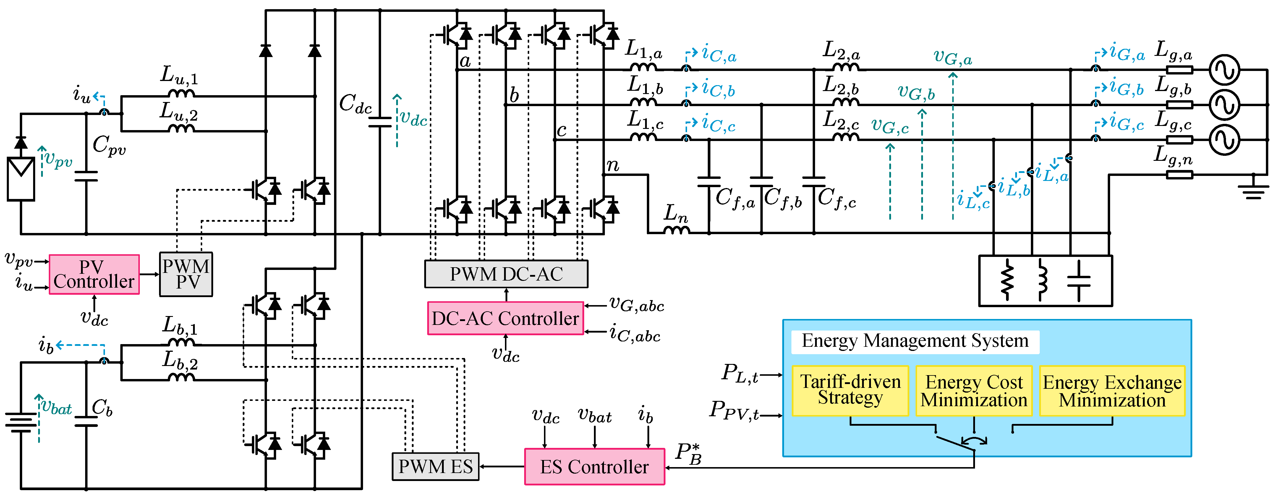
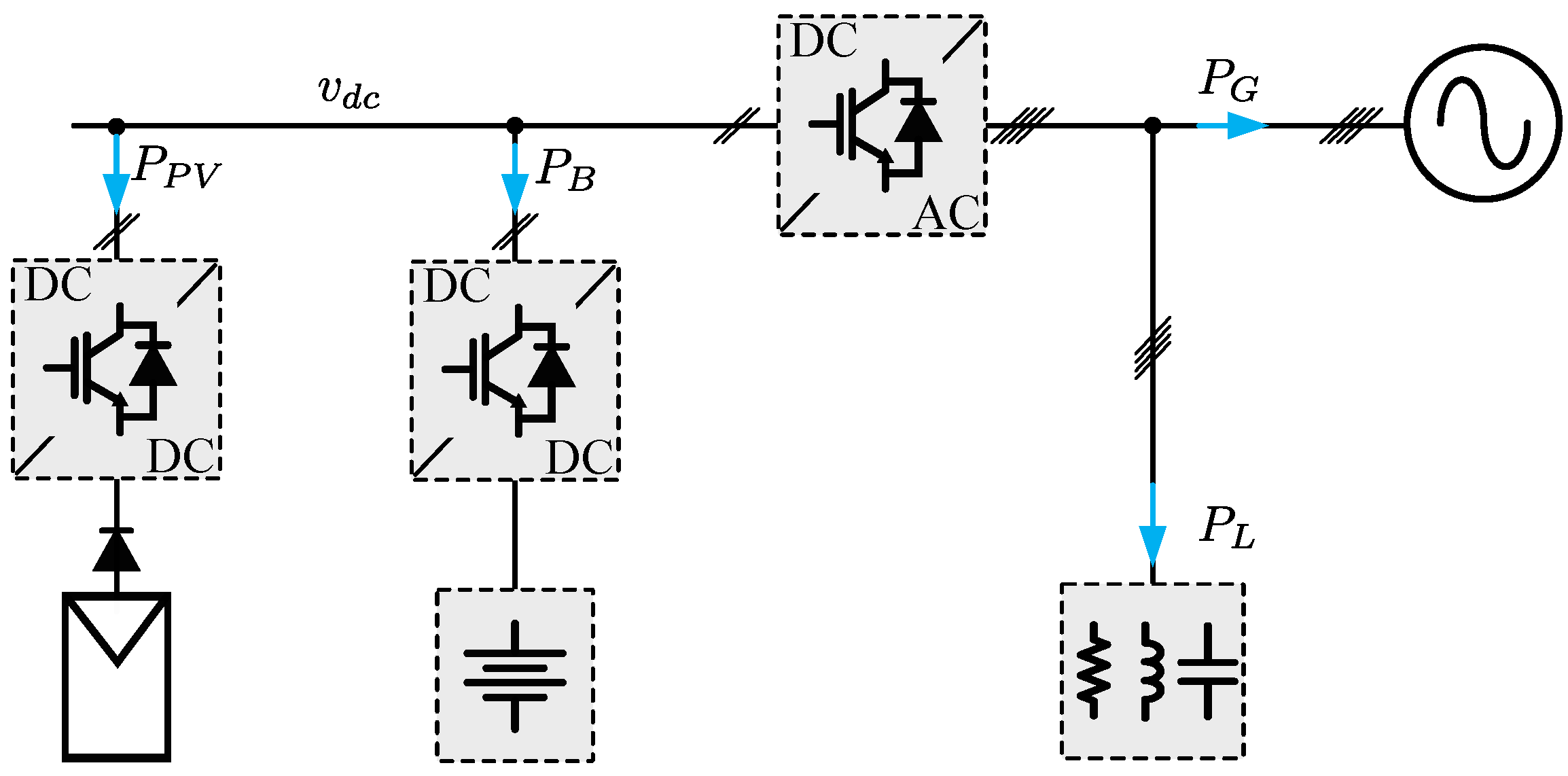
2. System Description

A residential grid-connected system with PV as a generation source and lithium-ion battery as the ES device is considered for this study and shown in Figure 1. The PV module is connected with a boost converter and the battery is interfaced to the DC bus with a bidirectional converter. Both of the DC-DC converters operate in the interleaving mode. This topology is selected because it reduces the current rating for the semiconductors. Besides, compared to the conventional converter, the filter size is reduced four times, obtaining the same input current ripple [32,33].
For the DC-AC stage, four-leg or three-leg two-level converters may be used depending on the load or mode of operation. However, in a residential context, power is supplied by a low-voltage distribution network, in which several single-phase loads or unbalanced three-phase loads are connected. Under this situation, to allow for increased flexibility and future operation in standalone mode with the capability to handle the zero-sequence components, a four-leg two-level converter with an LCL filter is used as the DC-AC stage to interface the grid with the supply system, compared to the three-leg converter that can only regulate positive and negative sequence components [34]. The grid impedance has been modeled with a configurable three-phase voltage source and lumped impedance with a value corresponding to the line length between the PCC and the nearest transformer in a given low-voltage distribution network. The parameters of the system under consideration are summarized in Table 1.
The following measurements are used either for the controllers or to calculate the power of the different energy exchange units in the system:
  • v p v —PV voltage,
  • i u —PV converter input current,
  • v b a t —battery voltage,
  • i b —battery converter input current,
  • v d c —DC bus voltage,
  • i C , a b c —DC-AC converter current,
  • i L , a b c —load currents,
  • v G , a b c —grid phase voltages at the PCC.
The EMS uses the expected power generation, P P V , t and load power demand P L , t for two days, producing as output the reference power for the battery P B * as shown in Figure 1. Even though the grid is available at all times, one can distinguish different operating scenarios depending on the energy exchange within the system.

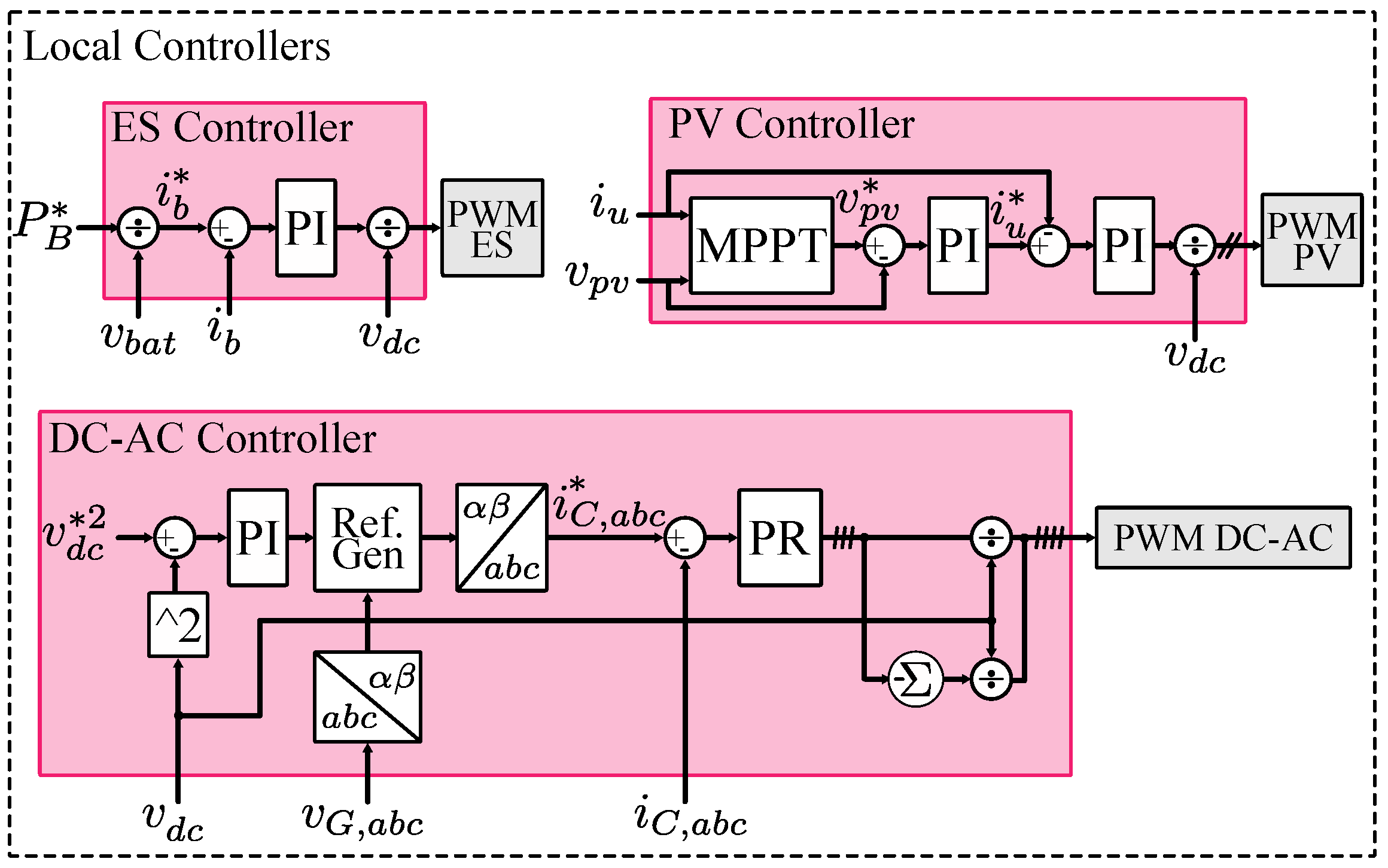
2.1. Local Controllers

The structure of local controllers for each device of the system is shown in Figure 2. The PV system controller is responsible for the generation of maximum available power. Therefore, a Maximum Power Point Tracking (MPPT) method sets the reference voltage v p v * at which the output power is maximum [35]. Then, the reference PV voltage v p v * is sent to an outer PI controller to set the reference current i u * , for the inner PI controller. The calculated output is then scaled by the DC bus voltage v d c to set the modulating signal of the converter.
The DC-AC converter controller regulates the DC bus voltage v d c and produces sinusoidal currents at the output. An outer PI controller is used to regulate the DC bus voltage. Then, the output of the controller and the measurements of the grid voltage v G , a b c is used to generate the reference currents i C , a b c * . It is important to mention that the reference currents are calculated to operate at the unity power factor. To track these reference currents, a Proportional Resonant (PR) controller is used for each phase, and the output is divided by the DC bus voltage v d c to send the resulting signal to the modulation stage of the inverter.
The input to the ES controller is the desired reference power for the battery P B * , which is later converted to the battery reference current i b * dividing it by the battery voltage v b a t . A PI controller is fed with the reference current i b * , and the output of the controller is scaled to produce the modulating signal for the bidirectional converter. This results in the control of charging and discharging cycles of the battery with the reference power P B * that is generated from the EMS. The details of the controllers implementation and their respective gains are summarized in Table 2. The transfer function that defines the PI controller is G P I s , and G P R s corresponds to the PR controller, where ω 0 = 2 π f g .

2.2. Operating Scenarios

A simplified diagram to describe the power balance of the system is shown in Figure 3, and the following considerations are taken into account:
  • system is considered lossless;
  • grid power, P G , is negative when the grid provides power to the loads and/or the battery, and positive when receiving power from the PV and/or the ES;
  • load power, P L , is always positive;
  • PV system power, P P V , is either negative or equal to zero;
  • power from the battery, P B , is positive when charging and negative when discharging.
The system under consideration operates in ten different modes, listed in Table 3. For any given scenario, (+) and (−) signs indicate power consumption and generation, respectively, while (0) denotes that power transfer is unavailable. In the case of PV installations they cannot produce power (0) if strings are covered (e.g., by snow) or there are dark clouds. The ES cannot provide energy (0 power available) if it is fully discharged or it cannot store more energy if it is fully charged. The operation details are discussed below for each configuration.
(1)
M1: The loads and the ES are supplied by the grid; this is applicable when the prices are low and it is desired to charge the battery. For this mode, the power balance is given by:
P G = ( P L + P B )
(2)
M2: In this case, the ES and the grid supply the power demanded by the loads. This scenario is possible when no PV generation is available, and it is intended to reduce the power demanded from the grid side.
(3)
M3: In this operating mode, the ES supplies both the loads and the grid. This scenario is expected at night hours when there is no PV generation or when the energy selling prices are high.
(4)
M4: In this case, the grid solely provides the power demanded by the loads, and the power balance is approximated as:
P G = P L
(5)
M5: This operating mode is related to the event where the PV can not fully supply the loads and charge the battery at the desired rate, resulting in the compensation of power from the grid. The power balance is approximated as:
P G = ( P L + P B + P P V )
(6)
M6: In this mode, the PV generation is greater than the demand for the loads and the battery, as a result, the excedent power is taken by the grid.
(7)
M7: This is the case when the PV is working in MPPT mode, and the ES is supplying power at the maximum limit and this does not suffice to supply the power demanded from the load. Then, the grid needs to provide additional power. This may be caused by a large demand from the loads and/or a low PV generation event.
(8)
M8: In this case, the generation from the residential system comes from the PV and ES, being greater than the load demand. The excess power is supplied to the grid, which may take place for local power demand or high power availability from the PV.
(9)
M9: This case results from the PV generation being lower than the load demand, for example, during night hours. This mode is similar to M6, with the difference of the ES being unable to store more energy. The power balance for this operation mode is given by:
P G = ( P L + P P V )
(10)
M10: In the last mode, the PV generation is greater than the load demand; consequently, the grid absorbs a surplus of power, since the ES cannot store more energy.
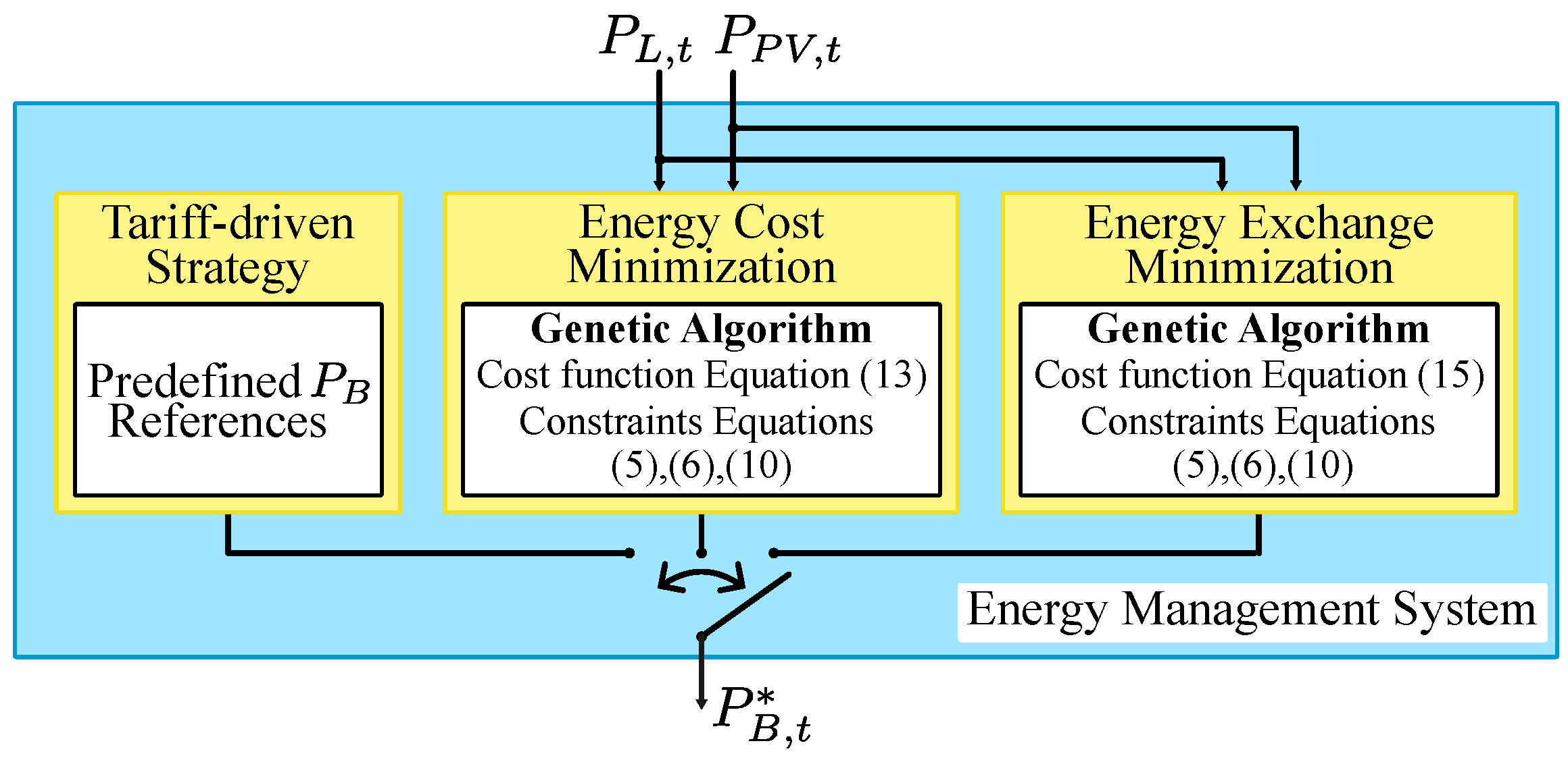
3. Proposed EMS

In Figure 4, three strategies for the EMS are shown. A simple tariff-driven strategy is proposed to have a comparison as a baseline. Additionally, two strategies that involve an optimization problem, namely, energy cost minimization and energy exchange minimization, are included. It is important to highlight that each objective is addressed separately. Therefore, this study does not address combinations of different energy management strategies, as the focus of this study is the comparison between the strategies under different generation conditions. This is different from a multiobjective optimization approach in which the optimization-based strategies can be combined.

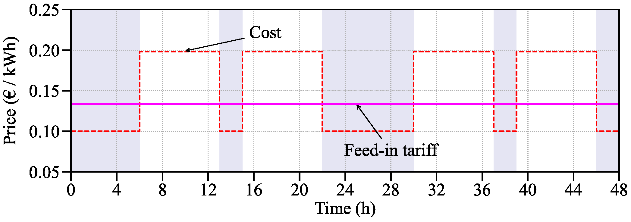
3.1. Tariff-Driven Strategy

The tariff-driven strategy can be implemented in a TOU tariff scenario, and the operation is as follows. During the day, the aim is to charge the battery at a constant rate during the timeframe in which the prices are cheaper to achieve the highest possible SOC before higher electricity prices begin. Then, when the cost of energy is higher, the battery is discharged at a constant rate before transitioning to the period when the energy is cheaper again. Usually, the last hours of the TOU scenario offer reduced prices, which can be leveraged to reach the desired SOC at the end of the day.

3.2. Energy Cost Minimization

The optimization of the total energy cost during two days has been proposed. For this strategy, the load and PV generation power profiles and the price rates are considered to be known in advance. Furthermore, a fixed rate per kWh is assumed when selling energy to the grid. In order to reduce the number of decision variables, the predicted generation and load profiles are averaged for a given time horizon. In this case, one hour is selected as the averaging period. Before solving the optimization problem, the objective function and constraints of the problem must be set.

3.2.1. Constraints

This strategy aims to minimize the total cost of the energy exchanged, and this must be conducted while guaranteeing a safe operation of the system. Therefore, the following constraints are set:
  • Maximum power limit: In order to avoid battery degradation, the battery must be charged/discharged, according to the manufacturer’s specification. For ES products that are available in the market, the continuous power rating of lithium-ion batteries is about 5 kW [36]. This constraint is described in (5).
    P B , m i n P B , t P B , m a x
The powers P B , m i n and P B , m a x , correspond to the minimum and maximum continuous power. In this case, the values are set to 5 kW and 5 kW, respectively.
  • Last value of SOC: To guarantee the operation of the system for the subsequent days, taking into consideration the next day’s forecast, an additional constraint is chosen where the target is to set the SOC at the end of the day to a predefined value, this constraint is expressed as:
    t = 1 k Δ S O C t + S O C 0 = S O C k
The index k corresponds to the hour chosen to reach a given SOC, for this case, two equality constraints are needed, one for the last hour of each day. Δ S O C t is the change in SOC at time t, and can be approximated by:
Δ S O C t = P B , t · Δ t C b a t
where C b a t is the total capacity of the ES and Δ t is the considered time step, in this case, one hour.
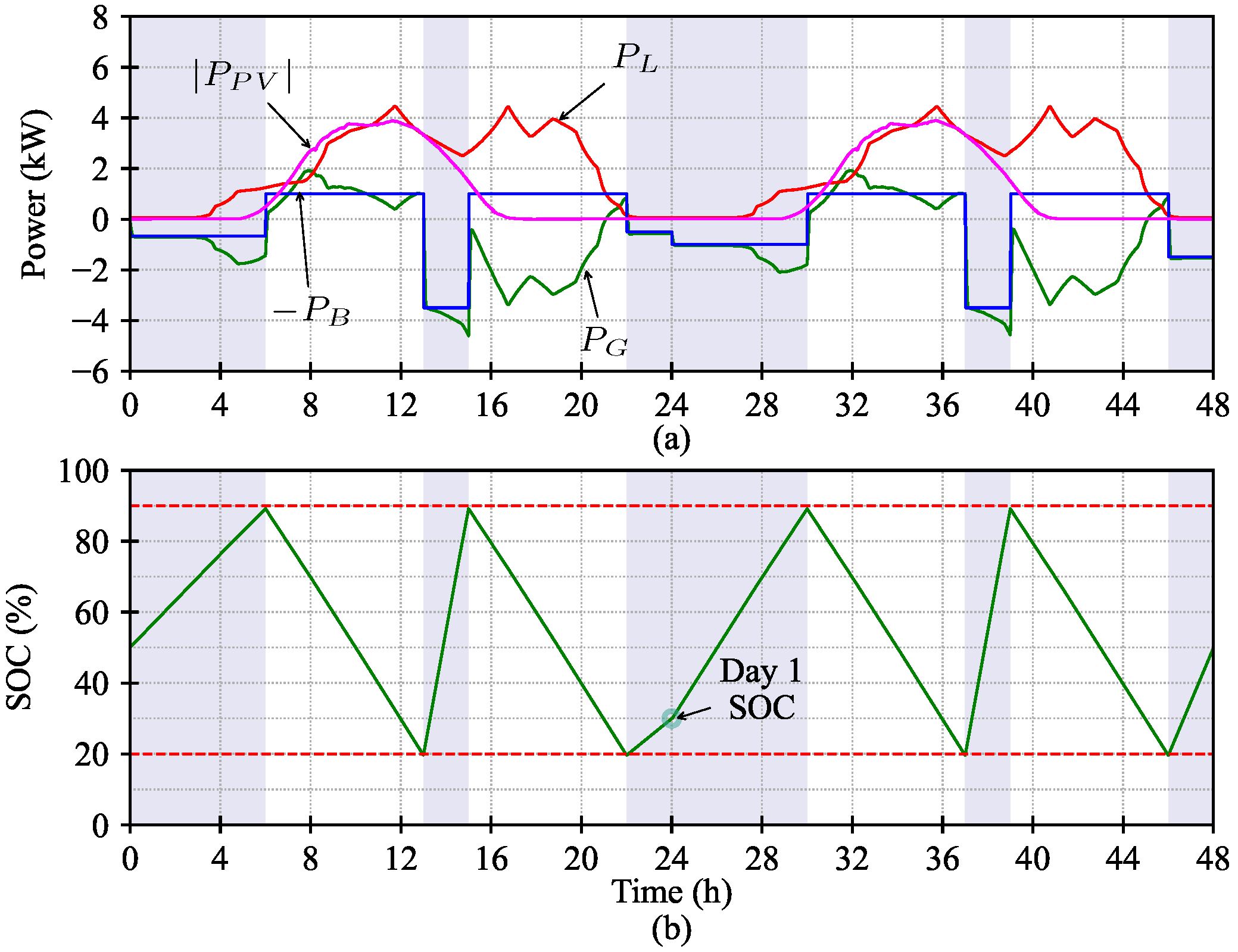
  • SOC limits: The following constraints are needed to guarantee that the SOC is within bounds during operation. For lithium-ion batteries, a lower limit of 20% is set, as a preventive measure to reduce the effect of aging due to a large depth of discharge (DOD) range [37]. A constant voltage control is needed to fully charge the battery, and this operating mode can be disregarded if the maximum SOC is set at 90%. In this range, the battery can safely operate in the continuous current charging/discharging mode. For the first hour of operation, the constraint is given by:
    S O C m i n S O C 0 + Δ S O C 1 S O C m a x
    For the first two hours of operation of the system, the constraint is given by:
    S O C m i n S O C 0 + Δ S O C 1 + Δ S O C 2 S O C m a x
Therefore, a total of 23 constraints for each day are needed to guarantee that the SOC is within limits during operation, and can be written as:
S O C m i n S O C 0 + t = 1 T = { 1 , 2 , , 23 } Δ S O C t S O C m a x
The constraints to keep the SOC within bounds at the last hour of each day (when t = 24 and t = 48 ) are taken into account with (6).

3.2.2. Cost Function

The objective of the problem is to minimize the total cost of energy in two days. A TOU tariff is considered when purchasing energy, and a fixed price is used for selling energy to the grid. When the power of the grid is negative, the incurred cost will depend on the TOU tariff; when the grid power is positive, the system owner gets revenue at a fixed price. Then, the cost function can be written as:
f = t = 1 48 P G , t · Δ t · c P G , t , t
where P G , t is the grid power, Δ t is the averaging period in hours (in this case, one hour), and c ( P G , t , t ) is a coefficient that is a function of the grid power and time. It can be modified to different scenarios, for example, variable rates of purchasing and feed-in tariffs. For this particular case, it is defined as:
c P G , t , t = 0.1   / kWh if P G , t < 0 , and { t 6 or 13 < t 15 or 22 < t 24 } 0.2   / kWh , P G , t < 0 , and { 6 < t 13 or 15 < t 22 } 0.13   / kWh , P G , t > 0 0   / kWh , P G , t = 0
If the power is positive, the coefficient is the feed-in tariff rate at which the energy is sold. On the contrary, when the power is negative, the value of the coefficient c P G , t , t is assigned according to the TOU rate. As previously mentioned, the hourly averaged generation and load profiles are available, using (3) and replacing it in (11), results in:
f = t = 1 48 ( P P V , t + P B , t + P L , t ) · Δ t · c ( P G , t , t )
In this form, the decision variable is the hourly reference power for the battery P B , t * , which is sent to the ES controller.

3.3. Energy Exchange Minimization

In order to provide another functionality and compare optimization approaches, a different objective is formulated, that is, the minimization of the grid energy exchange. The advantage of energy minimization is the ability to reduce power fluctuations, which is important for weak grids that are more sensitive to these conditions, resulting in degraded power quality. In order to guarantee the safe operation of the system, the same constraints as in the cost minimization approach are used, and a different cost function is formulated.

3.3.1. Cost Function

If the absolute value of the grid power at each time ( P G , t ) is minimized, then adding these values along the two days will minimize the energy exchange, and the cost function to achieve the objective is expressed as:
g = t = 1 48 | P G , t |
The grid power at a given time interval, P G , t , can be approximated with (3) and the cost function in which the target is to minimize the energy exchange results in:
g = t = 1 48 | ( P P V , t + P B , t + P L , t ) | · Δ t
Similar to the cost minimization strategy, the decision variable is the hourly power reference for the battery, P B * , which is sent to the ES controller.

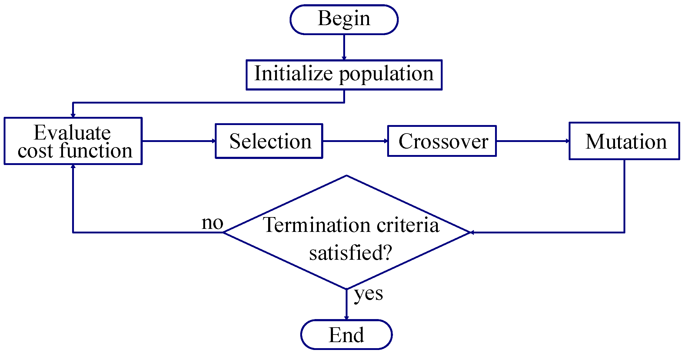
3.4. Genetic Algorithm

From the previous section, it can be noted that the cost functions are non-linear. For the energy cost minimization, the selling rates of the energy are defined by a piecewise linear function, that also depends on the grid power, P G , t and time t. Likewise, for the energy minimization objective, the cost function takes the absolute value of the grid power. Although metaheuristic methods such as GA can fall in a local minimum, their performance yields acceptable results compared with other methods [38]. On top of that, the use of metaheuristic algorithms is not restricted to a certain type of cost function or constraints, which provides additional flexibility. The primary goal of this study is the comparison of energy storage management techniques in single-objective formulation, a later study will make use of the methods available for multiobjective optimization for further comparison.
GA is in the class of metaheuristic optimization algorithms that are inspired by natural behavior and mimic a biological process, in this case, natural selection. This algorithm is flexible as it can deal with different problems compared to other approaches that are suitable only for specific cases. Besides, the GA provides a continuous search space for the multivariable problem, and it has a randomization component in the process that helps to explore other solutions and minimizes the possibility of getting stuck in local minimum [39]. The flowchart of the algorithm is presented in Figure 5, and the description of the algorithm applied to the problem being solved is the following:
  • Initial population: A number of individual solutions, N p , are created. The individual solution is a vector that has every component of the decision variable, in this case, the battery power for each hour, P B , 1 48 . For this particular problem, the constraints are linear, and the initial population is created so that each individual of the population satisfies the constraints [40].
  • Evaluate cost function: In this step each individual is evaluated in the cost function, (13) for cost minimization or (15) for energy exchange minimization.
  • Selection: As a result of the previous step, individual solutions yield different results. The best solutions are kept in the population and are duplicated, and the remaining ones are ruled out.
  • Crossover: In this step, new solutions are created, with probability p c , from combinations of a pair of individuals. In other words, two different solutions of battery power references ( P B , 1 48 ) are selected and combined to create a new solution.
  • Mutation: The purpose of this operation is to allow for exploration of the search space to escape from the local minimum. Some of the components of the individual (battery power references) are changed with probability p m . The operation is performed so the individual satisfies the constraints.
  • Termination criteria: Up to this step, one iteration of the algorithm has concluded. For this study, a predefined number of iterations N i , is selected as the termination criteria. If the number of iterations is reached, then the best solution from the population is selected.
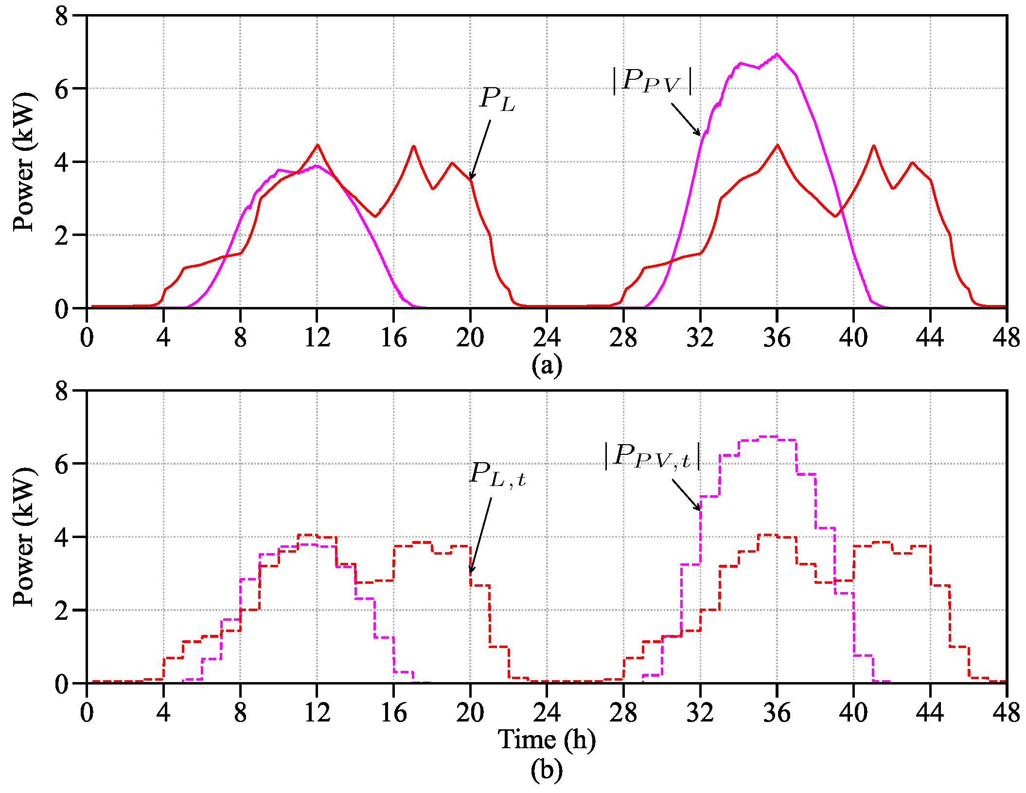
4. Case Study

The presented strategies have to be calculated ahead of time to schedule the battery’s power profile, setting an hourly power reference P B , t * , which is updated each hour and sent to the ES system controller. The SOC of the battery was calculated utilizing the “Coulomb count” method.
The collection of power profile data is facilitated by widely employed smart meters, which enable data acquisition with a resolution ranging from 15 min to one hour [41]. For simplicity, in this proposal, the averaged load and generation profiles have a resolution of one hour. Moreover, it is important to highlight that this method can be extended to a desired time window by easily adjusting the corresponding set of constraints and providing the data of power profiles accordingly. Besides, the cost minimization strategy can also handle dynamic tariffs, for example, with a resolution of one hour. Profiles with shorter resolution times as shown in Figure 6a are averaged on an hourly basis, resulting in the profiles that are illustrated in Figure 6b, the latter are used as inputs to the optimization problems, i.e., for the cost minimization and energy exchange minimization. It is important to note that the selected profiles represent two different scenarios. For the first 24 h a low PV generation profile is used, which can be considered to happen on cloudy days. On the other hand, for the last 24 h a sunny day is represented. In both cases, it can be noted that the peak power generation occurs in the middle hours of each day, and the load from the evening hours is not covered, which is a typical scenario. Regardless, these profiles can be changed accordingly to a specific location or scenario.
A TOU scenario is selected in order to compare the presented strategies, where two fixed rates, day and night tariffs, are available during the day. Both the cost at which the energy is purchased from the grid and the feed-in tariff are shown in Figure 7.
The energy management strategies discussed in Section 3, have been implemented and later tested in a detailed model where the PECs and their local controllers are included. Although the averaged power profiles were used as inputs in the optimization stage, the continuous load and PV generation profiles, which are shown in Figure 6a, were used during the tests to compare the energy management strategies.
Each strategy is tested for two consecutive days under four different power profiles: two consecutive days of cloudy or sunny profiles, and the scenarios where one of the days is sunny and the other is cloudy. For each of the EMS strategies and power profiles, three options for SOC at the end of the first day were set at 30%, 50%, and 90%, resulting in 36 studied scenarios. The starting and ending SOC is set at 50% in all the tests, and the target SOC at the end of the first day is modified to investigate which is the best option considering different power profiles.

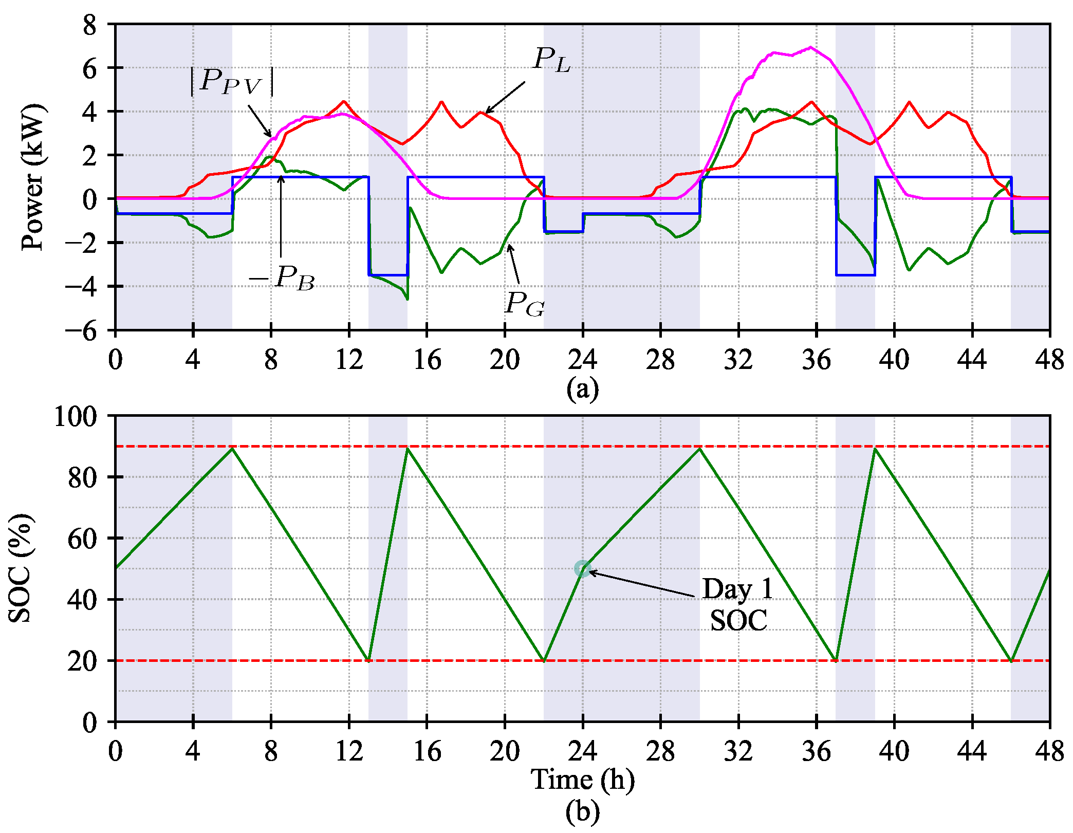
4.1. Tariff-Driven Strategy

Results for a target SOC of 30% and two cloudy days are presented in Figure 8. Night tariff periods are shaded in blue, while the day tariff period (higher prices) corresponds to the non-shaded area. The power profiles of the first day sunny and the second cloudy, and the SOC profile of the battery are presented in Figure 9a and Figure 9b, respectively. In this case, the target SOC at the end of the first day is set to 50%.
It is worth noting that in all cases the power profile of the battery and the SOC is the same for the first day, up to the last two hours. The battery power profile is not determined by the generation or load power profiles.

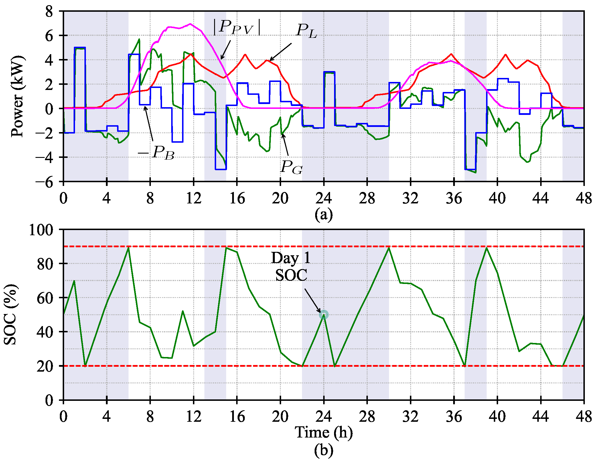
4.2. Energy Cost Minimization

Results for the scenario where the total cost of energy is minimized when the first day is sunny and the second day is cloudy are shown in Figure 10. Additionally, the setting for SOC target at the end of the day is set to 50%. Results regarding the scenario in which the first day is cloudy and the second day is sunny, with a setting for the SOC of 30% at the end of the first day are shown in Figure 11a, for the power profiles and Figure 11b for the SOC.
It is interesting to note that for the two scenarios shown, the battery is fully charged before the beginning of the period when the TOU tariff is high. This behavior is similar to the tariff-driven strategy proposed for comparison. Besides, it is observed that regardless of the target SOC and power profile, the battery is charged mostly during low-price hours, compared to the discharging events that occur when energy is more expensive.

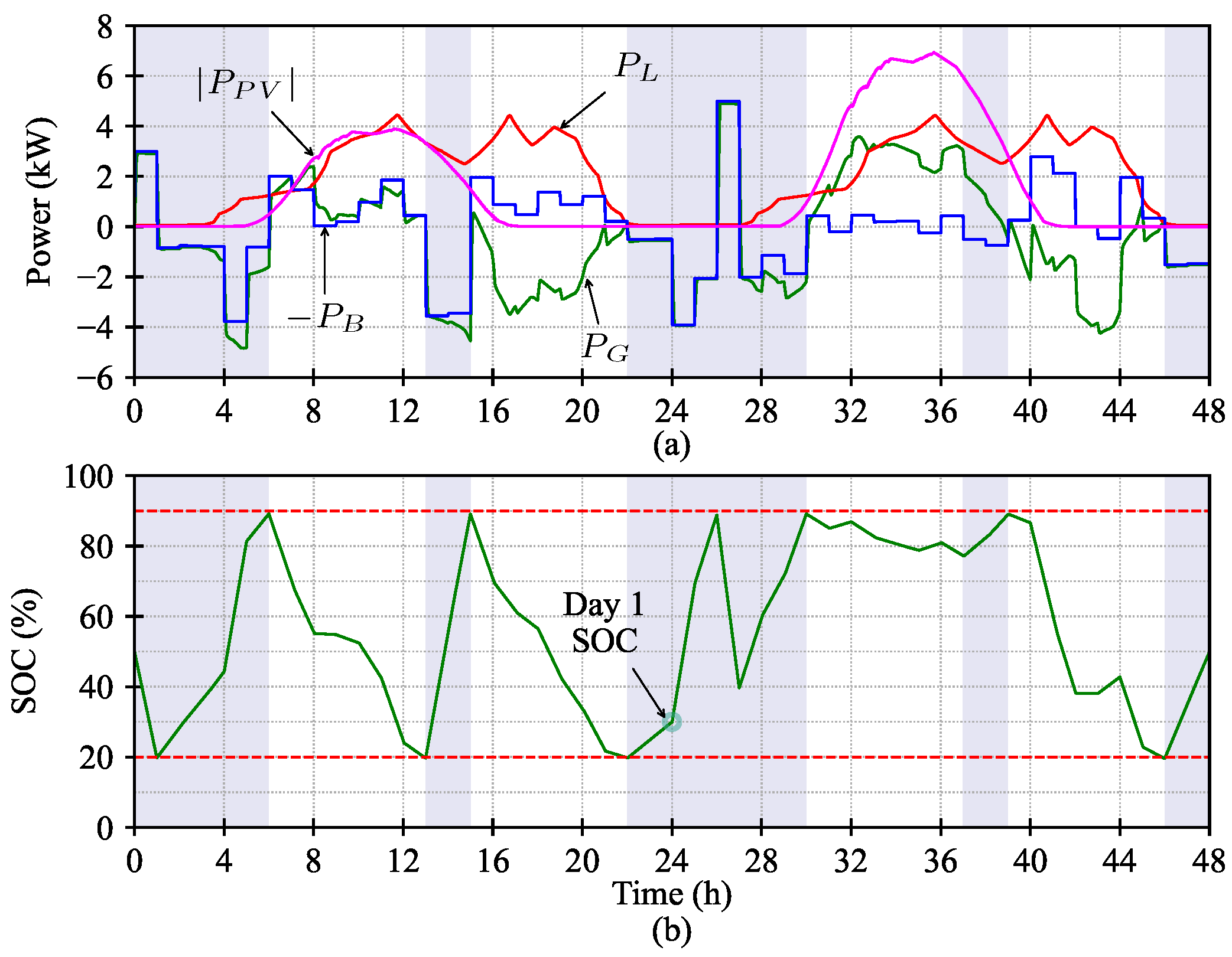
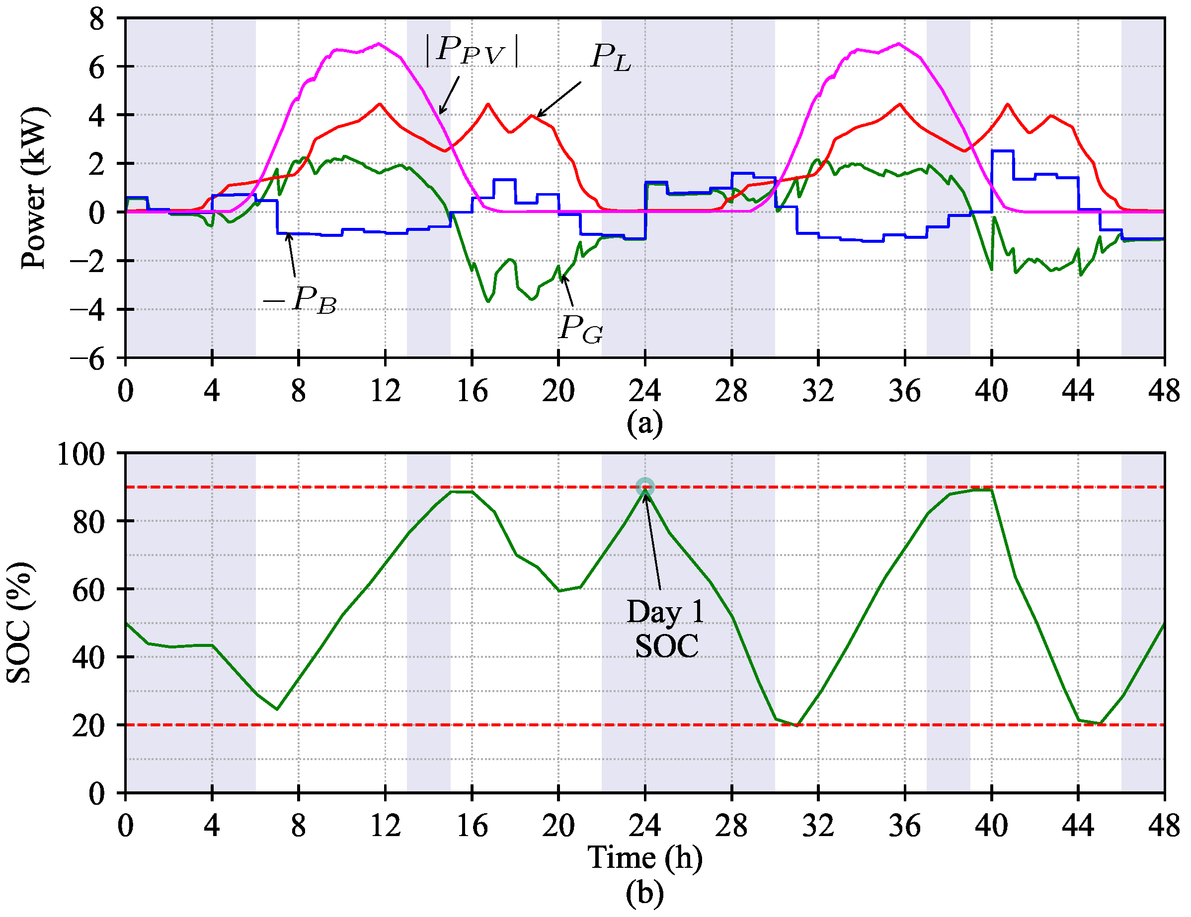
4.3. Energy Exchange Minimization

To demonstrate the performance of the system under the energy exchange minimization strategy, a new set of tests was carried out. The power profiles of the system for two sunny days, and the SOC profile of the battery are presented in Figure 12a and Figure 12b, respectively. In this case, the target SOC at the end of the first day is set to 90%. Additionally, the power profiles of the system are shown in Figure 13a for the scenario in which the first day is cloudy and the remaining 24 h corresponds to a sunny day, for a target SOC of 50%. Besides, the transitions of the SOC for this case are shown in Figure 13b.
The charging and discharging cycles of the battery are not related to the prices of the energy during the day. However, it is observed that when the energy exchange minimization strategy is used, the SOC profiles are smoother compared to the approach of cost minimization.

4.4. Comparison

A total of 36 scenarios were studied, i.e., three energy management strategies, for each strategy four different power profiles and for each power profile, three SOC targets at the end of the first day to study the influence of the final SOC value of the day. The starting and ending SOC of the 48 h analysis is the same for all cases and is set at 50%. The cost, total energy exchange, and peak power for each scenario and EMS strategy are summarized in Table 4.
The minimum cost is always achieved using the cost minimization strategy for a given power profile and target SOC at the end of two days. However, one of the key findings of this study is that for a given power profile, the target SOC that reduces the cost is different, as highlighted in green color in Table 4. For instance, for two cloudy days, the cost is minimized if the SOC at the end of the first day is 50%. In contrast, for the same power profile, the worst scenario in terms of cost is when the target SOC at the end of the day is 90% because more energy is taken to charge the battery under low irradiation conditions.
When the first day is cloudy and the second is sunny, the best economic result is achieved for the SOC setting at the end of the first day at 90%, which is explained because, at the end of the day, there is a low load profile and the tariffs used as a case study allow to sell the energy at a higher price than it was bought. On the other hand, under this generation profile the worst case in terms of cost, occurs when the target SOC is 30%. For the cases where the first day is sunny and the second is cloudy, or when the two days are sunny, the minimum cost is achieved when the target SOC is set at 30%, and the cost is increased when setting the target SOC to 90% and 50% for the sequence sunny-cloudy and two sunny days, respectively. For any scenario under a given power generation profile and target SOC, the total energy exchange is reduced almost two times compared to the cost minimization approach. Regardless of the generation power profile and SOC target in all cases, the energy is minimized when the SOC is set to 30% while the maximum energy exchange occurs when setting the SOC at the end of the day at 90%. Compared to the other strategies, for energy minimization, the positive peak power is minimized in all cases, and the negative peak power is reduced, except when the power profile is of two sunny days and the target SOC is 90%. On the contrary, when cost minimization is pursued, the maximum and minimum power of the grid are higher compared to the other strategies.

5. Conclusions

The development and implementation of energy management strategies have been presented: tariff-driven strategy, energy cost minimization, and energy exchange minimization. A given SOC level at the end of the day is achieved, providing better initial conditions of the ES for the next day’s operation. The tariff-driven strategy to charge/discharge the battery during low/high prices of energy has been proposed as a baseline to compare the optimized solutions. With this approach, the number of cycles of the battery is independent of the load and PV power profiles and is the same regardless of the final SOC.
Two residential system functionalities that use an optimization technique were implemented; for one case, the objective was to minimize the energy cost, and for the other scenario, the goal was to minimize the energy exchange with the grid during operation under different power generation profiles. For each of the above-mentioned strategies, three scenarios were tested considering different levels for the final SOC of the day as a constraint, specifically 30%, 50%, and 90%, comparing the benefits of flexible SOC settings based on the next day forecast. Additionally, a GA is used to solve the optimization problem, allowing for a continuous search space of solutions.
The energy management strategies were compared in terms of the total cost, the total energy exchange, and the maximum and minimum grid power. It is worth mentioning that reaching a minor SOC at the end of the first day does not produce a minimized cost in all cases. A different value of SOC should be selected at the end of the day depending on the PV generation power profiles of two consecutive days, and the final SOC cannot be neglected in the optimization process. Therefore, the SOC at the end of the day can also be optimized in the following research of the considered functionalities, based on next-day forecast and pre-calculated optimized benefits (minimized cost or energy exchange). Moreover, this study makes use of an offline single-objective optimization method, which is prone to diminished performance in the case when the forecast data change abruptly. Besides, the flexibility of the system could be further leveraged by controlling the local loads of the residential system. In consequence, future work will focus on implementing an online optimization method and the addition of demand-side management, considering controllable loads for additional flexibility, and the implementation of a multi-objective optimization algorithm to handle both objectives. Finally, a later implementation of the case study in a real-time platform will be carried out.

Author Contributions

Conceptualization, L.M.-C., R.K., A.M. and M.M.; methodology, L.M.-C.; software, L.M.-C., R.K. and A.M.; validation, L.M.-C.; formal analysis, L.M.-C.; investigation, L.M.-C., R.K. and A.M.; writing—original draft preparation, L.M.-C., R.K. and A.M.; writing—review and editing, L.M.-C., R.K., A.M. and M.M.; supervision, R.K., A.M. and M.M. All authors have read and agreed to the published version of the manuscript.

Funding

This project has received funding from the European Union’s Horizon 2020 research and innovation program under the Marie Skłodowska-Curie grant agreement No. 955614.

Data Availability Statement

Data are contained within the article.

Conflicts of Interest

The authors declare no conflict of interest. The funders had no role in the design of the study; in the collection, analyses, or interpretation of data; in the writing of the manuscript; or in the decision to publish the results.

Abbreviations

The following abbreviations are used in this manuscript:
AABCAdaptive artificial bee colony
AIArtificial intelligence
DERDistributed energy resource
DODDepth of discharge
DPDynamic programming
DSODistribution system operator
EMSEnergy management system
ESEnergy storage
GAGenetic algorithm
MILPMixed integer linear programming
MPCModel predictive control
MPPTMaximum power point tracking
NLPNon-linear programming
PCCPoint of common coupling
PECPower electronics converter
PRProportional resonant
PSOParticle swarm optimization
PVPhotovoltaic
QPQuadratic programming
RESRenewable energy source
SCSupercapacitor
SOCState of charge
TOUTime of use
WTWind turbine

References

  1. Fetting, C. The European Green Deal; Technical Report; ESDN Office: Vienna, Austria, 2020. [Google Scholar]
  2. Stynski, S.; Luo, W.; Chub, A.; Franquelo, L.G.; Malinowski, M.; Vinnikov, D. Utility-Scale Energy Storage Systems: Converters and Control. IEEE Industrial Electron. Mag. 2020, 14, 32–52. [Google Scholar] [CrossRef]
  3. Martins, J.F.; Romero-Cadaval, E.; Vinnikov, D.; Malinowski, M. Transactive Energy: Power Electronics Challenges. IEEE Power Electron. Mag. 2022, 9, 20–32. [Google Scholar] [CrossRef]
  4. García Vera, Y.E.; Dufo-López, R.; Bernal-Agustín, J.L. Energy Management in Microgrids with Renewable Energy Sources: A Literature Review. Appl. Sci. 2019, 9, 3854. [Google Scholar] [CrossRef]
  5. Hossain, M.A.; Pota, H.R.; Squartini, S.; Abdou, A.F. Modified PSO Algorithm for Real-Time Energy Management in Grid-Connected Microgrids. Renew. Energy 2019, 136, 746–757. [Google Scholar] [CrossRef]
  6. Ahmadiahangar, R.; Karami, H.; Husev, O.; Blinov, A.; Rosin, A.; Jonaitis, A.; Sanjari, M.J. Analytical Approach for Maximizing Self-Consumption of Nearly Zero Energy Buildings- Case Study: Baltic Region. Energy 2022, 238, 121744. [Google Scholar] [CrossRef]
  7. Zhao, Z.; Keerthisinghe, C. A Fast and Optimal Smart Home Energy Management System: State-Space Approximate Dynamic Programming. IEEE Access 2020, 8, 184151–184159. [Google Scholar] [CrossRef]
  8. Ruiz-Cortés, M.; González-Romera, E.; Amaral-Lopes, R.; Romero-Cadaval, E.; Martins, J.; Milanés-Montero, M.I.; Barrero-González, F. Optimal Charge/Discharge Scheduling of Batteries in Microgrids of Prosumers. IEEE Trans. Energy Convers. 2019, 34, 468–477. [Google Scholar] [CrossRef]
  9. González-Romera, E.; Ruiz-Cortés, M.; Milanés-Montero, M.I.; Barrero-González, F.; Romero-Cadaval, E.; Lopes, R.A.; Martins, J. Advantages of Minimizing Energy Exchange Instead of Energy Cost in Prosumer Microgrids. Energies 2019, 12, 719. [Google Scholar] [CrossRef]
  10. Thirunavukkarasu, G.S.; Seyedmahmoudian, M.; Jamei, E.; Horan, B.; Mekhilef, S.; Stojcevski, A. Role of Optimization Techniques in Microgrid Energy Management Systems—A Review. Energy Strategy Rev. 2022, 43, 100899. [Google Scholar] [CrossRef]
  11. Trivedi, R.; Khadem, S. Implementation of Artificial Intelligence Techniques in Microgrid Control Environment: Current Progress and Future Scopes. Energy AI 2022, 8, 100147. [Google Scholar] [CrossRef]
  12. Hafiz, F.; Lubkeman, D.; Husain, I.; Fajri, P. Energy Storage Management Strategy Based on Dynamic Programming and Optimal Sizing of PV Panel-Storage Capacity for a Residential System. In Proceedings of the 2018 IEEE/PES Transmission and Distribution Conf. and Exposition (T&D), Denver, CO, USA, 16–19 April 2018; pp. 1–9. [Google Scholar] [CrossRef]
  13. Li, Y.; Peng, J.; Jia, H.; Zou, B.; Hao, B.; Ma, T.; Wang, X. Optimal Battery Schedule for Grid-Connected Photovoltaic-Battery Systems of Office Buildings Based on a Dynamic Programming Algorithm. J. Energy Storage 2022, 50, 104557. [Google Scholar] [CrossRef]
  14. Ratnam, E.L.; Weller, S.R.; Kellett, C.M. An Optimization-Based Approach to Scheduling Residential Battery Storage with Solar PV: Assessing Customer Benefit. Renew. Energy 2015, 75, 123–134. [Google Scholar] [CrossRef]
  15. Liu, K.; Sheng, W.; Li, Z.; Liu, F.; Liu, Q.; Huang, Y.; Li, Y. An Energy Optimal Schedule Method for Distribution Network Considering the Access of Distributed Generation and Energy Storage. IET Gener. Transm. Distrib. 2023, 17, 2996–3015. [Google Scholar] [CrossRef]
  16. Georgiou, G.S.; Christodoulides, P.; Kalogirou, S.A. Optimizing the Energy Storage Schedule of a Battery in a PV Grid-Connected nZEB Using Linear Programming. Energy 2020, 208, 118177. [Google Scholar] [CrossRef]
  17. Härtel, F.; Bocklisch, T. Minimizing Energy Cost in PV Battery Storage Systems Using Reinforcement Learning. IEEE Access 2023, 11, 39855–39865. [Google Scholar] [CrossRef]
  18. Duan, Y.; Zhao, Y.; Hu, J. An Initialization-Free Distributed Algorithm for Dynamic Economic Dispatch Problems in Microgrid: Modeling, Optimization and Analysis. Sustain. Energy Grids Netw. 2023, 34, 101004. [Google Scholar] [CrossRef]
  19. Zia, M.F.; Elbouchikhi, E.; Benbouzid, M. Microgrids Energy Management Systems: A Critical Review on Methods, Solutions, and Prospects. Appl. Energy 2018, 222, 1033–1055. [Google Scholar] [CrossRef]
  20. Yi, Z.; Dong, W.; Etemadi, A.H. A Unified Control and Power Management Scheme for PV-Battery-Based Hybrid Microgrids for Both Grid-Connected and Islanded Modes. IEEE Trans. Smart Grid 2018, 9, 5975–5985. [Google Scholar] [CrossRef]
  21. Merabet, A.; Tawfique Ahmed, K.; Ibrahim, H.; Beguenane, R.; Ghias, A.M.Y.M. Energy Management and Control System for Laboratory Scale Microgrid Based Wind-PV-Battery. IEEE Trans. Sustain. Energy 2017, 8, 145–154. [Google Scholar] [CrossRef]
  22. Mahmud, K.; Sahoo, A.K.; Ravishankar, J.; Dong, Z.Y. Coordinated Multilayer Control for Energy Management of Grid-Connected AC Microgrids. IEEE Trans. Industry Appl. 2019, 55, 7071–7081. [Google Scholar] [CrossRef]
  23. Tran, V.T.; Islam, M.R.; Muttaqi, K.M.; Sutanto, D. An Efficient Energy Management Approach for a Solar-Powered EV Battery Charging Facility to Support Distribution Grids. IEEE Trans. Ind. Appl. 2019, 55, 6517–6526. [Google Scholar] [CrossRef]
  24. González-Romera, E.; Roncero-Clemente, C.; Barrero-González, F.; Milanés-Montero, M.I.; Romero-Cadaval, E. A Comprehensive Control Strategy for Multibus Nanogrids With Power Exchange Between Prosumers. IEEE Access 2021, 9, 104281–104293. [Google Scholar] [CrossRef]
  25. Agnoletto, E.J.; Silva de Castro, D.; Neves, R.V.A.; Quadros Machado, R.; Oliveira, V.A. An Optimal Energy Management Technique Using the ϵ-Constraint Method for Grid-Tied and Stand-Alone Battery-Based Microgrids. IEEE Access 2019, 7, 165928–165942. [Google Scholar] [CrossRef]
  26. Roncero-Clemente, C.; Roanes-Lozano, E.; Barrero-González, F. A Multi-Criteria Computer Package-Based Energy Management System for a Grid-Connected AC Nanogrid. Mathematics 2021, 9, 487. [Google Scholar] [CrossRef]
  27. Luna, A.C.; Meng, L.; Diaz, N.L.; Graells, M.; Vasquez, J.C.; Guerrero, J.M. Online Energy Management Systems for Microgrids: Experimental Validation and Assessment Framework. IEEE Trans. Power Electron. 2018, 33, 2201–2215. [Google Scholar] [CrossRef]
  28. Jafari, M.; Malekjamshidi, Z.; Zhu, J.; Khooban, M.H. A Novel Predictive Fuzzy Logic-Based Energy Management System for Grid-Connected and Off-Grid Operation of Residential Smart Microgrids. IEEE J. Emerg. Sel. Topics Power Electron. 2020, 8, 1391–1404. [Google Scholar] [CrossRef]
  29. Arcos-Aviles, D.; Pascual, J.; Guinjoan, F.; Marroyo, L.; García-Gutiérrez, G.; Gordillo-Orquera, R.; Llanos-Proaño, J.; Sanchis, P.; Motoasca, T.E. An Energy Management System Design Using Fuzzy Logic Control: Smoothing the Grid Power Profile of a Residential Electro-Thermal Microgrid. IEEE Access 2021, 9, 25172–25188. [Google Scholar] [CrossRef]
  30. Khan, M.A.; Haque, A.; Kurukuru, V.S.B. Power Flow Management With Q-Learning for a Grid Integrated Photovoltaic and Energy Storage System. IEEE J. Emerg. Sel. Top. Power Electron. 2022, 10, 5762–5772. [Google Scholar] [CrossRef]
  31. Chen, S.Y.; Chang, C.H. Optimal Power Flows Control for Home Energy Management With Renewable Energy and Energy Storage Systems. IEEE Trans. Energy Convers. 2023, 38, 218–229. [Google Scholar] [CrossRef]
  32. Sakasegawa, E.; Chishiki, R.; Sedutsu, R.; Soeda, T.; Haga, H.; Kennel, R.M. Comparison of Interleaved Boost Converter and Two-Phase Boost Converter Characteristics for Three-Level Inverters. World Electr. Veh. J. 2023, 14, 7. [Google Scholar] [CrossRef]
  33. Kroičs, K.; Staņa, Ģ. Bidirectional Interleaved DC–DC Converter for Supercapacitor Energy Storage Integration with Reduced Capacitance. Electronics 2023, 12, 126. [Google Scholar] [CrossRef]
  34. Rojas, F.; Cárdenas, R.; Burgos-Mellado, C.; Espina, E.; Pereda, J.; Pineda, C.; Arancibia, D.; Díaz, M. An Overview of Four-Leg Converters: Topologies, Modulations, Control and Applications. IEEE Access 2022, 10, 61277–61325. [Google Scholar] [CrossRef]
  35. Kot, R.; Stynski, S.; Stepien, K.; Zaleski, J.; Malinowski, M. Simple Technique Reducing Leakage Current for H-Bridge Converter in Transformerless Photovoltaic Generation. J. Power Electron. 2016, 16, 153–162. [Google Scholar] [CrossRef]
  36. Tesla Powerwall 2 Datasheet. Available online: https://www.tesla.com/sites/default/files/pdfs/powerwall/Powerwall%202_AC_Datasheet_en_northamerica.pdf (accessed on 13 June 2023).
  37. Han, X.; Lu, L.; Zheng, Y.; Feng, X.; Li, Z.; Li, J.; Ouyang, M. A Review on the Key Issues of the Lithium Ion Battery Degradation among the Whole Life Cycle. eTransportation 2019, 1, 100005. [Google Scholar] [CrossRef]
  38. Gelleschus, R.; Böttiger, M.; Stange, P.; Bocklisch, T. Comparison of Optimization Solvers in the Model Predictive Control of a PV-battery-heat Pump System. Energy Procedia 2018, 155, 524–535. [Google Scholar] [CrossRef]
  39. Katoch, S.; Chauhan, S.S.; Kumar, V. A Review on Genetic Algorithm: Past, Present, and Future. Multimed. Tools Appl. 2021, 80, 8091–8126. [Google Scholar] [CrossRef]
  40. Importance of Population Diversity, MATLAB. Available online: https://www.mathworks.com/help/gads/population-diversity.html (accessed on 17 December 2023).
  41. Bu, F.; Dehghanpour, K.; Wang, Z. Enriching Load Data Using Micro-PMUs and Smart Meters. IEEE Trans. Smart Grid 2021, 12, 5084–5094. [Google Scholar] [CrossRef]
Figure 1. Residential system under study.
Electronics 13 00087 g001
Figure 2. Local controllers of PECs.
Electronics 13 00087 g002
Figure 3. Simplified diagram of power balance in the system.
Electronics 13 00087 g003
Figure 4. Detailed diagram of the EMS functionalities.
Electronics 13 00087 g004
Figure 5. GA flowchart.
Electronics 13 00087 g005
Figure 6. PV generation and load profiles. (a) Continuous profiles. (b) Averaged profiles.
Electronics 13 00087 g006
Figure 7. Rates of energy cost and feed-in tariff.
Electronics 13 00087 g007
Figure 8. Tariff-driven strategy for 30% target SOC during two cloudy days. (a) Power profiles. (b) SOC.
Electronics 13 00087 g008
Figure 9. Tariff-driven strategy for 50% target SOC with first day cloudy and second sunny. (a) Power profiles. (b) SOC.
Electronics 13 00087 g009
Figure 10. Energy cost minimization for 50% target SOC with first day sunny and second cloudy. (a) Power profiles. (b) SOC.
Electronics 13 00087 g010
Figure 11. Energy cost minimization for 30% target SOC with first day cloudy and second day sunny. (a) Power profiles. (b) SOC.
Electronics 13 00087 g011
Figure 12. Energy exchange minimization for 90% target SOC, and two sunny days. (a) Power profiles. (b) SOC.
Electronics 13 00087 g012
Figure 13. Energy exchange minimization for 50% target SOC, with first day cloudy and second day sunny. (a) Power profiles. (b) SOC.
Electronics 13 00087 g013
Table 1. System parameters.
ParametersSymbolValuesParametersSymbolValues
PV System Maximum Power P P V M P P T 10 kWPV Voltage at Maximum Power Point V M P P 450 V
PV Short Circuit Current I S C 18.5 ABattery Total Energy C b a t 10 kWh
Battery Nominal Voltage v B 450 VGrid Nominal Voltage (line-neutral) v G 230 V RMS
Grid Nominal Frequency f g 50 HzGrid Inductance L g 100 µH
Grid Resistance R g 120 m Ω Switching frequency f s w 40 kHz
DC bus nominal voltage V d c 750 VDC bus capacitor C d c 1 mF
C d c internal resistor R d c 10 m Ω Filter converter side inductor L 1 , L n 2 mH
L 1 and L n internal resistor R 1 , R n 10 m Ω Filter grid side inductor L 2 300 µH
L 2 internal resistor R 2 10 m Ω Capacitor filter C f 3 µF
C f internal resistor R f 10 m Ω Boost converter inductance L u 4 mH
L u internal resistor R u 10 m Ω Battery converter inductance L b 4 mH
L b internal resistor R b 10 m Ω PV capacitor C p v 5 µF
C p v internal resistor R p v 10 m Ω Battery capacitor C b 5 µF
C b internal resistor R b 10 m Ω ---
Table 2. Structure of the controllers and gains.
DescriptionEquationGains
Proportional Integral
Battery current controller K p , i b = 32 K i , i b = 5
PV current controller G P I s = K p , x + K i , x s K p , i p v = 10.5 K i , i p v = 640
PV voltage controller K p , v p v = 0.03 K i , v p v = 720
DC Bus voltage controller K p , v d c = 0.59 K i , v d c = 72
DC-AC current controller G P R s = K p r + K r s s 2 + ω 0 2 K p r = 80.4 K r = 600
Table 3. System operation modes in grid-connected configuration.
ModePVESGrid
M10+
M20
M30+
M400
M5+
M6++
M7
M8+
M90
M100+
Table 4. Total cost, energy, and peak power results for the 36 tested scenarios, best cases highlighted in green and worst cases highlighted in red.
EMS SOC 30% SOC 50% SOC 90%
Cost (€) EE (kWh) P MAX (kW) P MIN (kW) Cost (€) EE (kWh) P MAX (kW) P MIN (kW) Cost (€) EE (kWh) P MAX (kW) P MIN (kW)
Cloudy—Cloudy
T D −6.5175.231.93−4.61−6.5175.211.93−4.61−6.5175.221.93−4.61
C M −6.2684.904.89−4.72−6.1394.204.85−5.26−6.3681.304.92−5.19
E M −7.6544.590.18−2.87−7.6145.020.41−2.97−7.6646.710.74−3.29
Cloudy—Sunny
T D −3.6686.494.13−4.61−3.6686.494.13−4.61−3.6686.504.13−4.61
C M −3.4793.224.92−4.86−3.36102.415.55−6.08−3.18111.886.59−5.04
E M −4.5150.052.26−2.74−4.5551.232.33−2.90−4.6559.162.25−3.03
Sunny—Cloudy
T D −3.6686.534.14−4.58−3.6686.524.14−4.58−3.6586.514.14−4.57
C M −3.23107.796.84−5.07−3.3399.915.69−5.27−3.4096.734.93−5.52
E M −4.5451.432.12−2.97−4.5351.582.33−2.84−4.6555.212.16−2.92
Sunny—Sunny
T D −0.8197.814.14−3.28−0.8197.784.14−3.27−0.8097.804.14−3.59
C M −0.33122.175.72−5.05−0.46114.795.56−4.65−0.36118.717.72−5.15
E M −1.4855.532.27−2.64−1.5257.522.23−2.59−1.7366.402.31−3.69
E E : Energy Exchange, P M A X : Maximum grid power, P M I N : Minimum grid power, T D : Tariff-driven, C M : Cost minimization, E M : Energy minimization.
Disclaimer/Publisher’s Note: The statements, opinions and data contained in all publications are solely those of the individual author(s) and contributor(s) and not of MDPI and/or the editor(s). MDPI and/or the editor(s) disclaim responsibility for any injury to people or property resulting from any ideas, methods, instructions or products referred to in the content.

