An Accurate and Invertible Sketch for Super Spread Detection

Abstract

Super spread detection has been widely applied in network management, recommender systems, and cyberspace security. It is more complicated than heavy hitter owing to the requirement of duplicate removal. Accurately detecting a super spread in real-time with small memory demands remains a nontrivial yet challenging issue. The previous work either had low accuracy or incurred heavy memory overhead and could not provide a precise cardinality estimation. This paper designed an invertible sketch for super spread detection with small memory demands and high accuracy. It introduces a power-weakening increment strategy that creates an environment encouraging sufficient competition at the early stages of discriminating a super spread and amplifying the comparative dominance to maintain accuracy. Extensive experiments have been performed based on actual Internet traffic traces and recommender system datasets. The trace-driven evaluation demonstrates that our sketch actualizes higher accuracy in super spread detection than state-of-the-art sketches. The super spread cardinality estimation error is 2.6–19.6 times lower than that of the previous algorithms.

1. Introduction

Super spread detection in real-time is crucial for security monitoring, network measurement, and resource alignment [1,2,3]. In general, flow size and cardinality are two basic statistics of interest, from which a variety of traffic information can be extracted. The flow size is the number of elements (e.g., bytes, packets, and contents) in a flow, and flow cardinality is the number of distinct elements (e.g., distinct addresses and ports) in a flow. The most significant difference between flow size and flow cardinality is that estimating a flow spread demands the removal of duplicate elements; however, estimating the flow size does not. A flow refers to data traffic that has the same or similar characteristics. This paper focuses on super spread identification (super spread is a flow with high cardinality), which can be widely used for search trend detection, recommender systems, anomaly detection, and DDoS detection [4,5,6,7].

Many studies have been proposed to find heavy flows with large sizes and have achieved significant progress [8,9,10,11]. However, finding super spreads is a more challenging problem because of the difficulty of deleting duplicates. Many useful per-flow estimators with different theoretical precisions, such as bitmap [12], Linear Counter (LC) [13], LogLog (LL) [14], Adapt Counter (AC) [15], and HyperLogLog (HLL) [16] have been designed for various situations and datasets. However, allocating an estimator for each flow is impractical because the required memory always exceeds the available memory.

It is challenging to find super spreads in data streams with limited memory. It is not possible to keep track of all flows accurately considering that a considerable amount of memory will be wasted by the recording of large-scale data streams. One strategy uses a sampling method to count a small part of the flow according to its actual cardinality. M2D is one typical algorithm [17]; however, sampling strategies lose accuracy. Another strategy used in the design of the above data structure is called estimator sharing [7,18,19,20,21,22], which uses one cardinality estimator for multiple flows. Sketch is a type of probabilistic data structure widely used in the field of network measurement to record the frequency or estimate the cardinality of elements in multiple sets or streams, and sketch is usually much smaller than the input size. Sketch-based measurement is a passive measurement, which usually does not send any detection packets and does not cause additional network overhead. Sketch uses profiles to effectively store and retrieve the information of interest, thereby achieving the recording of the presence and volume information of active flows. Then, the majority vote algorithm (MJRTY) [23] is used to find the maximum cardinality flow from the estimator and server as a possible super spread. However, MJRTY does not work well if the cardinality of a super spread is not significantly larger than the other flows.

To fill this gap, we present a novel sketch, called SSD-AIS, for super spread detection that can accurately detect super spread and provide precisely estimated flow cardinality. SSD-AIS adopts MJRTY in each bucket to find the candidate super spread while maintaining a key, a pvote counter, and a nvote counter. The pvote counter in the bucket records the cardinality of the candidate flow while the nvote counter records the cardinality of the other flows, which are mapped to this bucket. SSD-AIS only keeps track of a small amount of super spread and the vast majority of small spread flows will merely increase the value of nvote.

To avoid small spreads from increasing too much in nvote and affecting the accuracy, we propose a power-weakening increment strategy in SSD-AIS to increase nvote, which creates an environment encouraging sufficient competition in the early stages of discriminating a super spread and amplifying the comparative dominance when the value of pvote is large. The probability of an nvote value increment decreases with the power as pvote increases. Meanwhile, various cardinality estimators can be plugged into the SSD-AIS. In summary, the main contributions we have made are as follows:

(1)

We proposed an innovative invertible sketch data structure called SSD-AIS for super spread detection with small memory demands, which guarantees accuracy. Meanwhile, SSD-AIS can provide an exact spread estimation for the super spread.

(2)

We presented a mathematical analysis of memory usage and insert time, and the expectation of cardinality for a super spread.

(3)

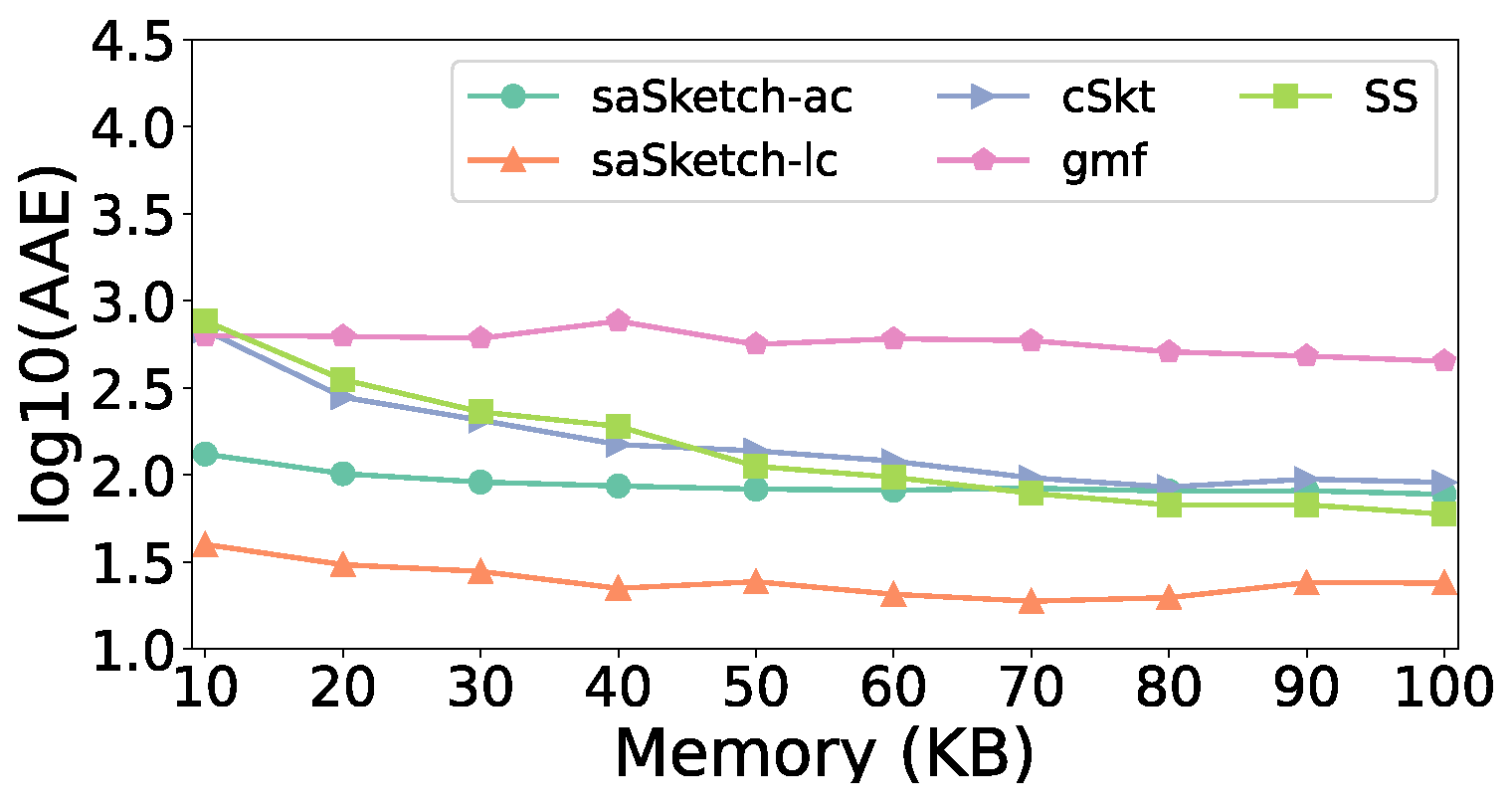
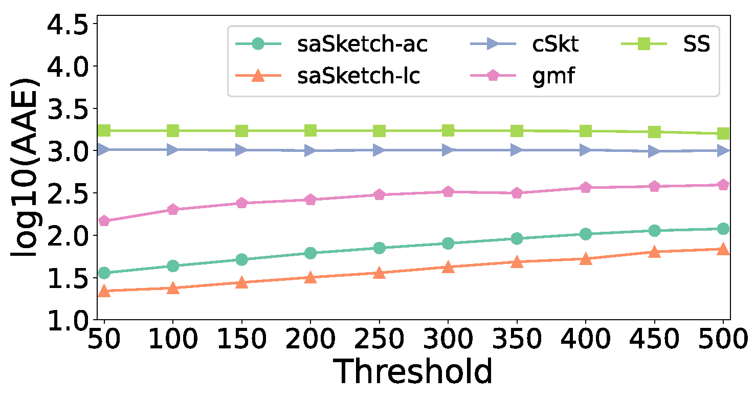
We implemented SSD-AIS with two standard cardinality estimators (AC and LC estimators). Trace-driven evaluations showed that SSD-AIS with the AC estimator and SSD-AIS with the LC estimator had higher accuracy in super spread detection compared to the state-of-art with small memory demands. And the average relative error of cardinality estimation of a super spread in SSD-AIS with the LC estimator is 2.6–19.6 times lower than the previous algorithms. The source code of SSD-AIS implementation and the related algorithms have been released at Github [24].

2. Related Works

In order to save memory, estimator sharing for multi-flow spread is widely adopted. Estimator sharing hashes each flow to $d$ estimators, each of which produces a spread estimation for flow $f$ independently. The smallest estimation carries the least error. There are two parts for one super spread: the value of cardinality and the flow label. Targeting the above two parts, existing approaches can be divided into two categories. Both of them have made certain progress in super spread detection; however, they also have deficiencies mainly in detection performance or resource expense (e.g., memory occupancy and detection accuracy). The distinct memory consumption of single estimator is presented in

Table 1. Memory costs for different estimators.

Estimator	Memory	Remark
Bitmap	m	m = n, n is the real cardinality of flow
Linear Counter	m	mln (m) > n
LogLog	32 m	Recommended as m = 128
Adaptive Counter	32 m	Recommended as m = 128
HyperLogLog	5 m	Recommended as m = 128

. The details are as follows.

Some approaches encode the flow label information into a sketch and then enumerate the entire label space to recover the candidate super spread. FAST [25] proposes an efficient data structure, namely, the fast sketch, which maintains multiple arrays of HLL sketches. For each arriving item, it splits flow label $f$ into two parts. One part has been hashed to a $d$ HLL array, and in each array records the element in one HLL. In this way, it can not only polymerize packets into a small number of flows but also further enable ISPs to discriminate the anomalous keys.

CDS [26] proposes a new data structure for locating the hosts associated with high connection degrees or significant variations in connection degrees based on the reversible connection degree sketch. It constructs a compact summary of host connection degrees, realizing an efficient and accurate analysis, and reconstructs the host addresses associated with large fan-outs by a simple computation merely based on the characteristics of the Chinese Remainder Theorem.

Vector Bloom Filter [27], which is a variant of the standard bloom filter, improves the update efficiency significantly via bit-extraction hashing. It can extract bits directly from the source ID and obtain the information of super spreads by using the overlapping of hash bit strings.

The approaches given above can find and derive super spreads; however, the computational cost is too high to afford the recovery of the flow label because the enormous flow label space and inaccuracy as an estimator have to be shared by many flows.

Some other approaches separate the cardinality and the flow label using existing frequency-based sketches to return high-frequency keys and use another data structure to store the flow label of the candidate super spread. cSkt [28] extended the Count-Min sketch [29] with an external heap for tracking super spreads and associated each bucket with a distinct cardinality estimator, which is simple and easy to implement.

OpenSketch [30], which offloads part of the measurement function to the data plane from the control plane, combined reversible sketch [31] with bitmap algorithms. In the data plane, it provides a simple three-stage pipeline involving hashing, filtering, and counting to implement measurement tasks of cardinality and flow labels. In the control plane, it provides a measurement library to realize automatic configurations of the pipeline and resource allocation for different measurement tasks.

And Liu [7] et al. combined Fast Sketch [25] with an optimal distinct counter for super spread detection. It designs a reversible and mergeable data structure for a distributed network monitoring system, which means implementing network traffic measurements at each local monitor and reporting high-cardinality hosts productively based on compressed information, thus avoiding querying every single host in the network.

The approaches above can find and derive the super spreads; however, existing invertible frequency-based sketches, as proposed above, have heavy processing overhead: either incurring high memory access overhead for heap updates or inducing an unaffordable update overhead that grows linearly with the key size.

Among them, gmf [26], and SpreadSketch [20] are two of the state-of-the-art implementations. The core technologies introduced by gmf are a generalized geometric counter, a generalized geometric hash function, and an innovative geometric minimum filter that can eliminate duplication and block the vast majority of mice or small streams. Therefore, after the original flow passes through the filter, only a small number of flows are tracked using the hash table. In this way, gmf separates a super spread from the vast majority of small flows. This method greatly reduces memory usage, but cannot accurately measure the cardinality of super spread.

SpreadSketch can simultaneously measure the diffusion of a lot of traffic and distinguish the super spreads among them. It extends the Count-Min [29] while replacing each counter with multi-resolution bitmaps, a label field, and a register [22]. The label field is used to record a flow label. However, if the cardinality of streams mapped to the same bucket is very close, especially when memory is small, its detection is not accurate enough.

In conclusion, although the above methods have made some progress in super spread detection, they cannot meet the requirements of accuracy and performance for super spread detection at the same time, especially when the cardinality of a super spread is not significantly larger than other spreads and the available memory is small (less than 100 KB). Besides, the cardinality they provide is not accurate enough.

3. Overview

In this section, we introduce the core idea behind SSD-AIS in the first place. We then present the data structure and basic operations of SSD-AIS. The notations frequently used in subsequent paragraphs of this paper and their meanings are listed in

Table 2. Notations.

Notations	Meanings
$S$	A data stream
$M$	The number of flows in $S$
$N$	32 m
$L$	32 m
$f_i$	5 m
$F_i$	The fingerprint of flow $f_i$
$n_i$	Real spread of flow $f_i$
$\dot{n_i}$	Estimated spread of flow $f_i$
$d$	Array number
$w$	The bucket number in an array
$\alpha$	Predefined parameter
$\beta$	Predefined parameter

.

3.1. Subsection

In the estimator-sharing method, multiple flows are hashed into the same estimator because the number of estimators is far less than the number of flows. Intuitively, we can adopt the majority vote algorithm (MJRTY) [23] to search the candidate super spread. MJRTY maintains a vote key and a vote counter in one bucket. When processing an element $e$, if $e$ is equal to the vote key, then the estimator is increased or decreased. By comparing with the vote key, the estimator can accurately find the element that repeatedly occurs for more than half of the elements of the input. In today’s network environment, online processing has become an important performance requirement. To provide an online spread estimation of a super spread, we use two estimators in one bucket: a pvote estimator and an nvote estimator. The pvote estimator counts and records the number of distinct elements of the candidate flow, and the nvote estimator counts and records the number of distinct elements of the other flows.

To find a super spread, there are two main problems we need to overcome when using MJRTY. First, the assumption of the application scenarios that the spread of a flow exceeding half of the spread of all flows hashed in this bucket is not always satisfied. Second, if two super spreads are mapped to one bucket, at least one of them will be underreported owing to the collision. However, this probability cannot be ignored when the number of buckets is small.

To address the first problem, we designed a power-weakening increment strategy for the nvote estimator inspired by the positive feedback of cybernetics. When an incoming element does not match the candidate key, we increase the nvote estimator with probabilities based on the value of the pvote estimator. For example, if the pvote value is 100 and the power is 2, the probability of an increment for nvote is ${(1/100)}^2$. The power-weakening increment strategy creates an environment encouraging sufficient competition in the early stages of discriminating a candidate super spread and the decay nvote estimator increases when the pvote estimator is large enough to ensure accuracy.

To address the second problem, we adopted the classical count-min sketch, which consists of multiple arrays. Count-Min sketch will hash any incoming item into a bucket in each array and increase the corresponding bucket. Finally, it returns the minimum values of all corresponding buckets as the estimated value of this item. In our design, we return the value of the corresponding buckets after checking whether the key in the bucket and item match. Assuming that the probability of two super spreads colliding in an array is $p$ and that the sketch is composed of $d$ arrays, then the probability that a super spread will eventually be stored in Sketch is greater than $1-p^d$. The probability of underreporting has been greatly reduced through a combination of sketches and MJRTY.

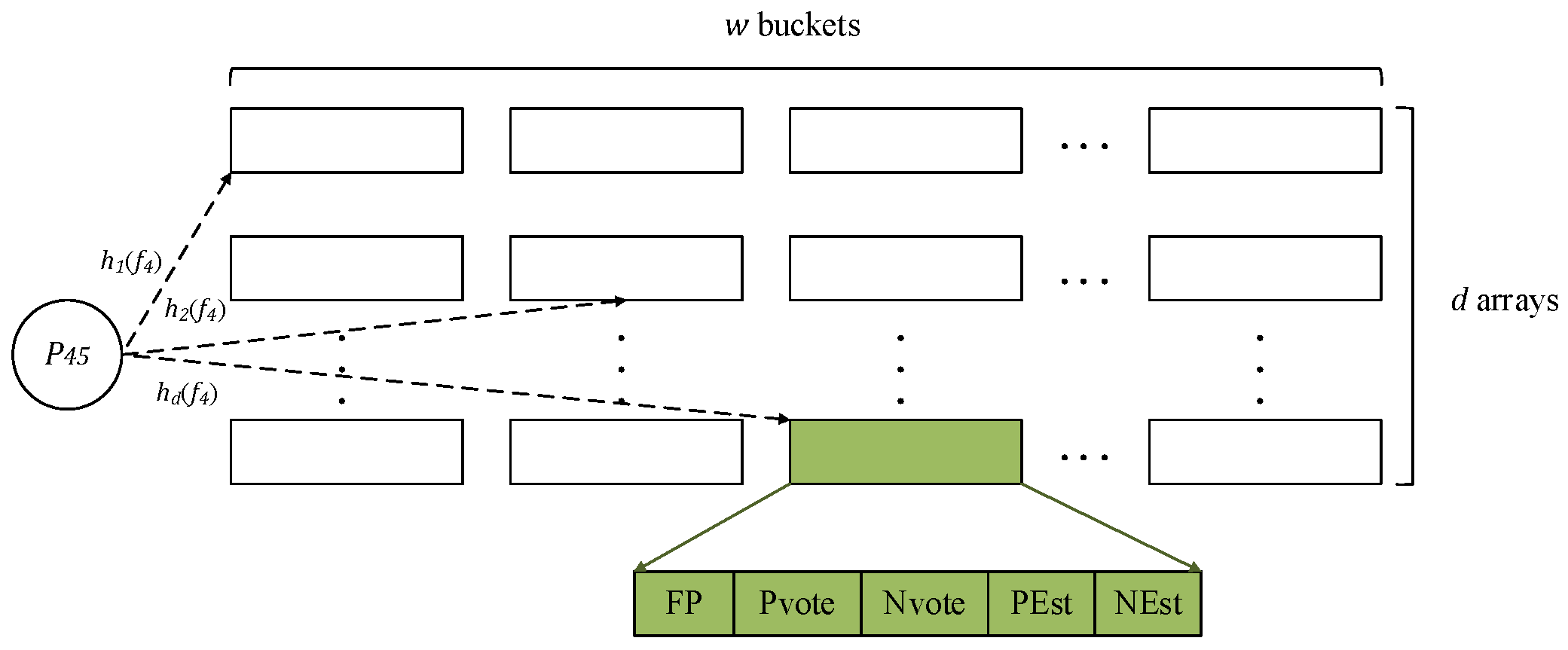
3.2. Data Structure

The data structure of SSD-AIS is composed of $d$ arrays, and each array has $w$ buckets, as shown in Figure 1. Each bucket has five fields: (1) an FP field storing the fingerprint of the candidate super spread in the bucket, (2) a PEst estimator storing the element of the candidate flow, (3) an NEst estimator counting the number of elements that have a different fingerprint from the candidate super spread in the bucket, (4) a pvote count record of the value of the PEs estimator, and (5) a nvote count record of the value of the NEst estimator. In addition, SSD-AIS has $d$ pairwise-independent hash functions, represented by ${\mathrm{h}}_1,{\mathrm{h}}_2,...,{\mathrm{h}}_{\mathrm{d}}$. And each hash function $h_i$ ($1\le i\le d$) hashes the flow label $f$ of each incoming item $〈f, e〉$ to one of the buckets in row $i$.

Note that many efficient spread estimators are suitable for different data and requirements, such as bitmap, LC, FM, LL, AC, and HLL. These estimators can be efficiently and simply combined with SSD-AIS as a plug-in. In other words, we generalize and combine the structure of SSD-AIS to a family of sketches, called saSketch, and provide a plug-in component method for a different estimator.

For convenience, we use $A\left[u\right]\left[v\right](0\le u<d,0\le v<w)$ to represent the v-th bucket in the u-th array. Then we use $A\left[u\right]\left[v\right].FP$, $A\left[u\right]\left[v\right].Pvote$, $A\left[u\right]\left[v\right].Nvote$, $A\left[u\right]\left[v\right].PEst$, and $A\left[u\right]\left[v\right].NEst$ to denote the FP field, pvote count, nvote count, PEst estimator, and NEst estimator in the bucket $A\left[u\right]\left[v\right]$, respectively. We use the action descriptions Increase (PEst) or Increase (NEst) to uniformly represent the item insertion into the estimator. For different estimators, the insertion methods are different. For example, the LC estimator is implemented as a bitmap and hash incoming item to a bit in the LC estimator and we set the bit to one.

3.3. Basic Operations

Initialization: All valuations of the fields in SSD-AIS are initially set as null or 0.

Insertion: The step-by-step pseudocode of the insertion operation is presented as Algorithm 1. For each incoming item $〈f_i, e_j〉$, the flow label is $f_i$ and the element label is $e_j$. In general, SSD-AIS computes $d$ hash functions and maps flow $f_i$ to $d$ bucket. For each row $u$, we first compute the hash function $h_u\left(f_i\right)$ to obtain the bucket position $v$ in the corresponding row. Based on the values of the corresponding fields in $A\left[u\right]\left[v\right]$, as shown in Figure 2, there are three different cases, as follows:

Case 1: When $A\left[u\right]\left[v\right].Pvote=0$. This means bucket $A\left[u\right]\left[v\right]$ is null, then SSD-AIS sets $A\left[u\right]\left[v\right].FP=F_i$ and increases $A\left[u\right]\left[v\right].PEst$.

Case 2: When $A\left[u\right]\left[v\right].Pvote>0$ and $A\left[u\right]\left[v\right].FP=F_i$. This means that the flow $f_i$ is the candidate super spread, then SSD-AIS increases $A\left[u\right]\left[v\right].Pvote$.

Case 3: When $A\left[u\right]\left[v\right].Pvote>0$ and $A\left[u\right]\left[v\right].FP\ne F_i$. This means that the flow $f_i$ is not the candidate super spread, and SSD-AIS increases $A\left[u\right]\left[v\right].NEst$ with a probability $P_{power}$. After increasing $A\left[u\right]\left[v\right].NEst$ and updating $A\left[u\right]\left[v\right].Nvote$, if $A\left[u\right]\left[v\right].Nvote$ is greater than or equal to $A\left[u\right]\left[v\right].Pvote$, SSD-AIS clears bucket $A\left[u\right]\left[v\right]$.

Algorithm 1: Insertion

$\hspace{1em}\mathbf{Input}: \mathrm{A} \mathrm{data} \mathrm{item} 〈f_i,e_j〉$  Output: update SSD-AIS $1 \hspace{1em}\mathbf{for} u\leftarrow$1 to d do $2 \hspace{1em}\hspace{1em}v\leftarrow h_u\left(f_i\right)$ mod w; $3 \hspace{1em}\hspace{1em}\mathbf{if} A\left[u\right]\left[v\right].Pvote=0$ then $4 \hspace{1em}\hspace{1em}\hspace{1em}A\left[u\right]\left[v\right].FP\leftarrow F_i$; $5 \hspace{1em}\hspace{1em}\hspace{1em}\mathit{Increase}\left(A\right[u\left]\right[v].Pvote$); $6 \hspace{1em}\hspace{1em}\hspace{1em}\mathit{Update}\left(A\right[u\left]\right[v].PEst$); $7 \hspace{1em}\hspace{1em}\mathbf{else} \mathbf{if} A\left[u\right]\left[v\right].FP=F_i$ then $8 \hspace{1em}\hspace{1em}\hspace{1em}\mathit{Increase}\left(A\right[u\left]\right[v].Pvote$); $9 \hspace{1em}\hspace{1em}\hspace{1em}\mathit{Update}\left(A\right[u\left]\right[v].PEst$); $10\hspace{1em}\hspace{1em}\mathbf{else}$ $11 \hspace{1em}\hspace{1em} P_{power}={\left(\frac{\beta }{A\left[u\right]\left[v\right].Pvote}\right)}^{\alpha }$; $12 \hspace{1em}\hspace{1em} \mathbf{if} rand\left(1\right)<P_{power}$ then $13 \hspace{1em}\hspace{1em}\hspace{1em} \mathit{Increase}\left(A\right[u\left]\right[v].Nvote$); $14 \hspace{1em}\hspace{1em}\hspace{1em} \mathit{Update}\left(A\right[u\left]\right[v].NEst$); $15 \hspace{1em}\hspace{1em}\hspace{1em} \mathbf{if} A\left[u\right]\left[v\right].Nvote\ge A\left[u\right]\left[v\right].Pvote$ then $16 \hspace{1em}\hspace{1em}\hspace{1em}\hspace{1em} \mathrm{clear} \mathrm{bucket} A\left[u\right]\left[v\right]$;

Note that probability is a very important parameter in the power-weakening increment strategy. Probability is defined as follows:

$$P_{power}={\left(\frac{\beta }{A[u][v].Pvote}\right)}^{\alpha }$$

(1)

where $\alpha$ and $\beta$ are predefined constant parameters (e.g., $\alpha =0.4,\beta =1$). It can be observed that $P_{power}$ decreases as $A\left[u\right]\left[v\right].Pvote$ increases. For a super spread, the corresponding pvote estimator in the bucket is incremented regularly, whereas the nvote estimator increases with a dynamic decrease probability. Therefore, SSD-AIS magnifies the relative advantage of the candidate super spread, and the accuracy of super spread detection is high.

Query: Given a threshold $\mathsf{\Phi }$, SSD-AIS returns super spread and the value of the spread whose spread exceeds $\mathsf{\Phi }$. The pseudocode of the operation in query process is presented in Algorithm 2. First, SSD-AIS traverses all buckets; if the pvote of a bucket is greater than the threshold $\mathsf{\Phi }$, add the FP to the unique set $S$. Then, SSD-AIS traverses the set $S$ using PointQuery (see Algorithm 3) to obtain the cardinality value of flow $f$($f\in S$). If the estimated spread $s$ exceeds threshold $\mathsf{\Phi }$, add $〈f, s〉$ to the super spread list $R$. Then, we get the potential super spreads.

Algorithm 2: Query process

$\hspace{1em} \mathbf{Input}: \mathrm{threshold} \mathsf{\Phi }$  Output:$\mathrm{A} \mathrm{set} S$$\mathrm{and} \mathrm{super} \mathrm{spread} \mathrm{list} R$ $1 \hspace{1em}\mathbf{for} u\leftarrow$1 to d do $2 \hspace{1em}\mathbf{for} v\leftarrow$1 to d do; $3 \hspace{1em}\hspace{1em}\mathbf{if} A\left[u\right]\left[v\right].Pvote\ge \mathsf{\Phi }$ then $4 \hspace{1em}\hspace{1em}\mathrm{add} A\left[u\right]\left[v\right].FP$ to set $S$ $5 \hspace{1em}\mathbf{for} \mathrm{each} f\in S$ do  $6 \hspace{1em}\hspace{1em}s\leftarrow PointQuery\left(f\right)$; $7 \hspace{1em}\hspace{1em}\mathbf{if} s\ge \mathsf{\Phi }$ then $8 \hspace{1em}\hspace{1em}\mathrm{add} <f,s>$ into $R$;

Algorithm 3: PointQuery

$\hspace{1em}\mathbf{Input}: \mathrm{flow} f$ $\hspace{1em}\mathbf{Output}: \mathrm{the} \mathrm{estimated} \mathrm{spread} s$ of flow $f$ $1 \hspace{1em}\mathbf{for} u\leftarrow$1 to d do $2 \hspace{1em}\hspace{1em}v\leftarrow h_u\left(f_i\right)$$\mathrm{mod} w$; $3 \hspace{1em}\hspace{1em}flag\leftarrow Flase$; $4 \hspace{1em}\hspace{1em}\mathrm{initial} s$ to a big value; $5 \hspace{1em}\hspace{1em}\mathbf{if} A\left[u\right]\left[v\right].FP=f$ then $6 \hspace{1em}\hspace{1em}s\leftarrow min(s,A[u\left]\right[v].Pvote)$; $7 \hspace{1em}\hspace{1em}flag\leftarrow True$; $8\hspace{1em}\hspace{1em}\mathbf{if} flag=True$ then $9 \hspace{1em}\hspace{1em}\mathrm{return} s$; 10  else 11     return 0;

4. Theoretical Analysis

4.1. Space and Time Complexities

Assume that the estimator in SSD-AIS is m-bit and that the time estimator update required is $t_e$. SSD-AIS has $dw$ buckets, each of which contains a log L-bit candidate flow label, two loglog L-bit level counters, and two m-bit estimators. Thus, the memory space occupied is $\mathrm{O}\left(dw\right(\mathrm{l}\mathrm{o}\mathrm{g} L+2\mathrm{l}\mathrm{o}\mathrm{g}\mathrm{l}\mathrm{o}\mathrm{g}L+2m\left)\right)$.

Each packet accesses $d$ bucket to update the estimator. Then, we use the returned result of the estimator to update Vote (pvote or nvote). Thus, the insertion time is $\mathrm{O}(d\cdot (t_e+1\left)\right)$.

4.2. Error Analysis

There are two main processes from real cardinality to the final estimated cardinality for a super spread. The first part is the transformation of real cardinality $n_i$ into the candidate super spread’s real cardinality $\overline{n_i}$ through the Majority Vote algorithm in SSD-AIS, and the second part is the transformation of the candidate super spread’s real cardinality $\overline{n_i}$ into the final estimated cardinality $\dot{n_i}$ by the estimator. The second part of the transformation depends on the estimator type, including its mean and standard deviation. In this paper, we mainly focus on the first part of the transformation.

There are two cases in the first part of the transformation as shown in Figure 3. In the first case, there are no waste items for the final candidate super spread. In other words, when the first item belonging to this super spread arrives at SSD-AIS, it becomes a candidate. In the second case, some thriftless items are wasted before the corresponding spread becomes a candidate super spread.

Theorem 1.

Assume that a candidate super spread is held at its mapped bucket all the time, which is described as case 1. Without a loss of generality, let us focus on one single array of SSD-AIS. Given a small positive value $\epsilon$ and a candidate super spread with flow label $f_i$,

$$\mathrm{Pr}(n_i-{\widehat{n}}_i\ge \epsilon N)<\frac{1}{\epsilon w}\cdot {\left(\frac{\beta }{\beta +1}\right)}^{\alpha }$$

(2)

Proof of Theorem 1.

We respectively prove case 1 and case 2.

Case 1: Firstly, we introduce indicator variable $I_{i, j, k}$, defined as:

$$I_{i,j,k}=\left\{\begin{array}{c}0\hspace{1em}\mathrm{if}(f_i=f_k)\vee (h_j(f_i)\ne h_j(f_k)\hfill \\ 1\hspace{1em}\mathrm{if}(f_i\ne f_k)\wedge (h_j(f_i)=h_j(f_k))\hfill \end{array}\right.$$

(3)

When $I_{i, j, k}=1$, it means two different flows $f_i$ and $f_k$ are mapped into the same bucket in the $j^{\mathrm{t}\mathrm{h}}$ array. Suppose that each flow is uniformly mapped to one of the $w$ counters randomly using the hash functions. The probabilities of the collision between two distinct flows are $\frac{1}{w}$, so the expectation of $I_{i, j, k}$ is as follows:

$$E(I_{i,j,k})=\mathrm{Pr}[h_j(f_i)=h_j(f_k)]=\frac{1}{\mathrm{range}(h_j)}=\frac{1}{w}$$

(4)

Then, we define the random variable $X_{i, j}$ as:

$$X_{i,j}={\displaystyle \sum _{k=1}^M{I}_{i,j,k}{n}_k}$$

(5)

$X_{i, j}$ refers to the summation of the sizes of other distinct flows mapped to the same bucket in row $j$, except for the flow $f_i$ itself. Then, the expectation of $X_{i, j}$ is:

$$\mathrm{E}(X_{i,j})=\mathrm{E}\left({\displaystyle \sum _{k=1}^M{I}_{i,j,k}{n}_k}\right)={\displaystyle \sum _{k=1}^M\left(E(I_{i,j,k})\cdot n_k\right)}=\frac{N-n_i}{w}$$

(6)

For each incoming packet, the value change depends on whether it belongs to the flow $f_i$: if so, the pvote is increased; if not, nvote increases with a certain probability. One extreme situation is that all packets that do not belong to the candidate flow increment the nvote, and then we have $\overline{n_i}=n_i-X_{i, j}$. Another extreme case is that all packets that do not belong to the candidate flow do not increase the nvote; then, we have $\overline{n_i}=n_i$. Therefore, we have:

$$n_i-X_{i,j}\le {\overline{n}}_i\le n_i$$

(7)

Next, a random variable $P_{i, j, l}$ is defined, representing the probability of the l-th packet in $X_{i, j},$ which increases the nvote. The incremental probability of nvote $P_{i, j, l}$ in the power-weakening strategy is defined as Formula (8):

$$P_{i,j,l}=\left\{\begin{array}{cc}1& \mathrm{if}\hspace{0.33em}{C}_l<\beta \\ {\left(\frac{\beta }{C_l}\right)}^{\alpha }& \mathrm{if}\hspace{0.33em}{C}_l\ge \beta \end{array}\right.$$

(8)

where $C_l$ represents the value of pvote when the l-th packet in $X_{i, j}$ arrives. We have:

$${\overline{n}}_i=n_i-{\displaystyle \sum _{l=1}^{X_{i,j}}{P}_{i,j,l}}$$

(9)

By the Markov inequality, the following formula holds:

$$\mathrm{Pr}(n_i-{\overline{n}}_i\ge \epsilon N)=\mathrm{Pr}({\displaystyle \sum _{l=1}^{X_{i,j}}{P}_{i.j.l}}\ge \epsilon N)\le \frac{E({\displaystyle {\sum }_{l=1}^{X_{i,j}}{P}_{i,j,l}})}{\epsilon N}$$

(10)

Then we focus on $E\left(\sum _{l=1}^{X_{i, j}}{P}_{i, j, l}\right)$. It is assumed that all packets are uniformly distributed. From Equation (8), we can obtain $P_{i, j, l}=1$ when $1\le C_l\le \beta$; thus, we have:

$$\mathrm{Pr}\{P_{i,j,l}=1\}=\frac{\beta }{\gamma }$$

(11)

For convenience, let $\gamma$ present $n_i-\sum _{l=1}^{X_{i,j}}{P}_{i,j,l}$. When $\beta <C_l\le n_i-E\left(\sum _{l=1}^{X_{i,j}}{P}_{i,j,l}\right)$, we have:

$$\mathrm{Pr}\{P_{i,j,l}={{\displaystyle \left(\frac{\beta }{C_l}\right)}}^{\alpha }\}=\frac{1}{n_i-E({\displaystyle {\sum }_{l=1}^{X_{i,j}}{P}_{i,j,l}})}=\frac{1}{\gamma }$$

(12)

As a result, the expectation of variable $P_{i, j, l}$ can be represented as:

$$\begin{array}{cc}\hfill E({\displaystyle \sum _{l=1}^{X_{i,j}}{P}_{i,j,l}})& ={\displaystyle \sum _{l=1}^{E(X_{i,j})}E(P_{i,j,l})}\hfill \\ \hfill & =E(X_{i,j})\left(\frac{\beta }{\gamma }+\frac{1}{\gamma }{{\displaystyle \sum _{C_l=\beta +1}^{\gamma }\left(\frac{\beta }{C_l}\right)}}^{\alpha }\right)\hfill \\ \hfill & \mathrm{because} \frac{\beta }{C_l}\le \frac{\beta }{\beta +1},\mathrm{when}\hspace{0.33em}{C}_l\in [\beta +1,\gamma ]\hfill \\ \hfill & \le E(X_{i,j})\left(\frac{\beta }{\gamma }+\frac{(\gamma -\beta )}{\gamma }{\left(\frac{\beta }{\beta +1}\right)}^{\alpha }\right)\hfill \end{array}$$

(13)

Focusing on the latter part, we have:

$$\begin{array}{l}\frac{\beta }{\gamma }+\frac{(\gamma -\beta )}{\gamma }{\left(\frac{\beta }{\beta +1}\right)}^{\alpha }\\ =\frac{1}{\gamma }\left\{\beta \cdot \left(1-{\left(\frac{\beta }{\beta +1}\right)}^{\alpha }+{\left(\frac{\beta }{\beta +1}\right)}^{\alpha }\right)+(\gamma -\beta )\cdot {\left(\frac{\beta }{\beta +1}\right)}^{\alpha }\right\}\\ =\frac{1}{\gamma }\left\{\gamma \cdot {\left(\frac{\beta }{\beta +1}\right)}^{\alpha }+\beta \cdot \left(1-{\left(\frac{\beta }{\beta +1}\right)}^{\alpha }\right)\right\}\\ \mathrm{because} \frac{\beta }{\beta +1}<1\\ <\frac{1}{\gamma }\left\{\gamma \cdot {\left(\frac{\beta }{\beta +1}\right)}^{\alpha }\right\}={\left(\frac{\beta }{\beta +1}\right)}^{\alpha }\end{array}$$

(14)

Based on Equation (6), we get:

$$E({\displaystyle \sum _{l=1}^{X_{i,j}}{P}_{i,j,l}})<\frac{N-n_i}{w}\cdot {\left(\frac{\beta }{\beta +1}\right)}^{\alpha }$$

(15)

Then combined with Equation (10), we have:

$$\begin{array}{cc}\hfill \mathrm{Pr}(n_i-{\overline{n}}_i\ge \epsilon N)& =\mathrm{Pr}({\displaystyle \sum _{l=1}^{X_{i,j}}{P}_{i.j.l}}\ge \epsilon N)\hfill \\ \hfill & \le \frac{E({\displaystyle {\sum }_{l=1}^{X_{i,j}}{P}_{i,j,l}})}{\epsilon N}\hfill \\ \hfill & <\frac{1}{\epsilon w}\cdot {\left(\frac{\beta }{\beta +1}\right)}^{\alpha }\hfill \end{array}$$

(16)

Case 2: We divided the real value of the super spread into two parts $n_i^1$ and $n_i^2$, where $n_i^1$ represents the wasted items before $f_i$ becomes the candidate flow, and $n_i^2$ represents the items after $f_i$ becomes the candidate flow. When $f_i$ becomes the candidate flow, the analysis is the same as in case 1. For the same reason, the number of all items $N$ is divided into two parts: $N_1$ and $N_2$. Then, we have:

$$\mathrm{Pr}(n_i^2-{\overline{n}}_i^2\ge \epsilon N_2)<\frac{1}{\epsilon w}\cdot {\left(\frac{\beta }{\beta +1}\right)}^{\alpha }$$

(17)

Because ${\overline{n_i}}^2$ is the final candidate super spread’s real value,

$${\overline{n}}_i^2={\overline{n}}_i$$

(18)

Combining Equations (17) and (18), we have:

$$\mathrm{Pr}({\overline{n}}_i\le n_i^2-\epsilon N_2)<\frac{1}{\epsilon w}\cdot {\left(\frac{\beta }{\beta +1}\right)}^{\alpha }$$

(19)

Then,

$$\begin{array}{cc}\hfill \mathrm{Pr}({\overline{n}}_i\le n_i-\epsilon N)& =\mathrm{Pr}({\overline{n}}_i\le n_i^1+n_i^2-\epsilon (N_1+N_2))\hfill \\ \hfill & <\mathrm{Pr}({\overline{n}}_i\le n_i^2-\epsilon N_2)\hfill \\ \hfill & <\frac{1}{\epsilon w}\cdot {\left(\frac{\beta }{\beta +1}\right)}^{\alpha }\hfill \end{array}$$

(20)

Combining Case 1 and Case 2, Theorem 1 holds.

Next, we consider the second part of the transformation. The LC estimator and AC estimators are both unbiased [13,15] and the expectation of the estimator is equal to the true value of the parameter being estimated, which is denoted as:

$$E({\widehat{n}}_i)={\overline{n}}_i$$

(21)

Therefore, the expectation of the estimated value has the following properties:

$$\mathrm{Pr}\left\{E({\widehat{n}}_i)\le n_i-\epsilon N\right\}<\frac{1}{\epsilon w}\cdot {\left(\frac{\beta }{\beta +1}\right)}^{\alpha }$$

(22)

□

5. Evaluation

In this section, three main performances that SSD-AIS achieved via trace-driven evaluation are shown as follows: (1) high accuracy in super spread detection, (2) low error in cardinality estimation, and (3) high processing speed with a small and static space.

5.1. Setup

Platform: The experiments we conducted were run on a server with four 18-core Intel Xeon Gold 5318Hs @2.5 GHz CPU and 256 GB DDR4 memory. The CPU has 1152 KB of L1 cache per core, and 24.75 MB of shared L3 cache.

Dataset:

(1)

Recommender System Dataset: The dataset used in the experiment was collected from a real-world e-commerce website [32] and we used the visitor behavior data. We took the item ID as the flow label and visitor ID as the element identifier. Then, there were approximately 2.7 M items and 200 k flows. The flow cardinality in this dataset is defined as the number of distinct visitors viewing the item, reflecting the popularity of the corresponding product.

(2)

CAIDA Dataset: This dataset contains anonymized IP traces collected in 2016 by CAIDA [33]. In this experiment, we considered the destination IP address as the flow label and all packets toward the same destination constituted a flow. The source IP address was used as the element identifier. The first 4 M packets of this dataset belonging to approximately 50 K flows were used in the experiment. The flow spread in this dataset is the number of distinct source IP addresses communicating with the same destination IP address, which may reflect the victims of the DDoS attack.

Implementation: We have implemented Geometric-Min Filter (gmf) [19], cSkt [28], SpreadSketch (SS) [20], SSD-AIS with an LC estimator (saSketch-lc), and SSD-AIS with an AC estimator (saSketch-ac).

gmf and saSketch-lc both use the LC estimator and an estimator with 200 bits. The length of the filter array in the gmf was 2000. saSketch-ac and cSkt both use the AC estimator, where the number of registers in each estimator is 128 and each register is 4 bits. The estimator in SpreadSketch is a multi-resolution bitmap, and the estimator is 438 bits according to [20]. All algorithms were implemented in C++. The hash functions we utilized in the above sketches are murmurhash32 Hash (obtained from the website [34]).

5.2. Metrics

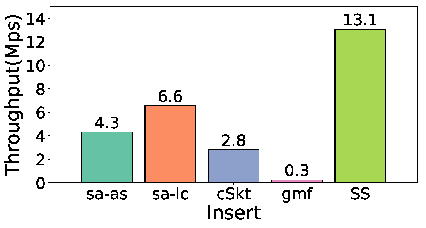
• Throughput: All packets are inserted and the corresponding throughput is calculated. The throughput is defined as $\mathrm{N}/\mathrm{T}$, where $\mathrm{T}$ represents the total processing time. The measuring method is inserting millions of packets per second and the unit of the throughput is Mps. We repeated the experiments 10 times and recorded and reported the average value of the throughput.
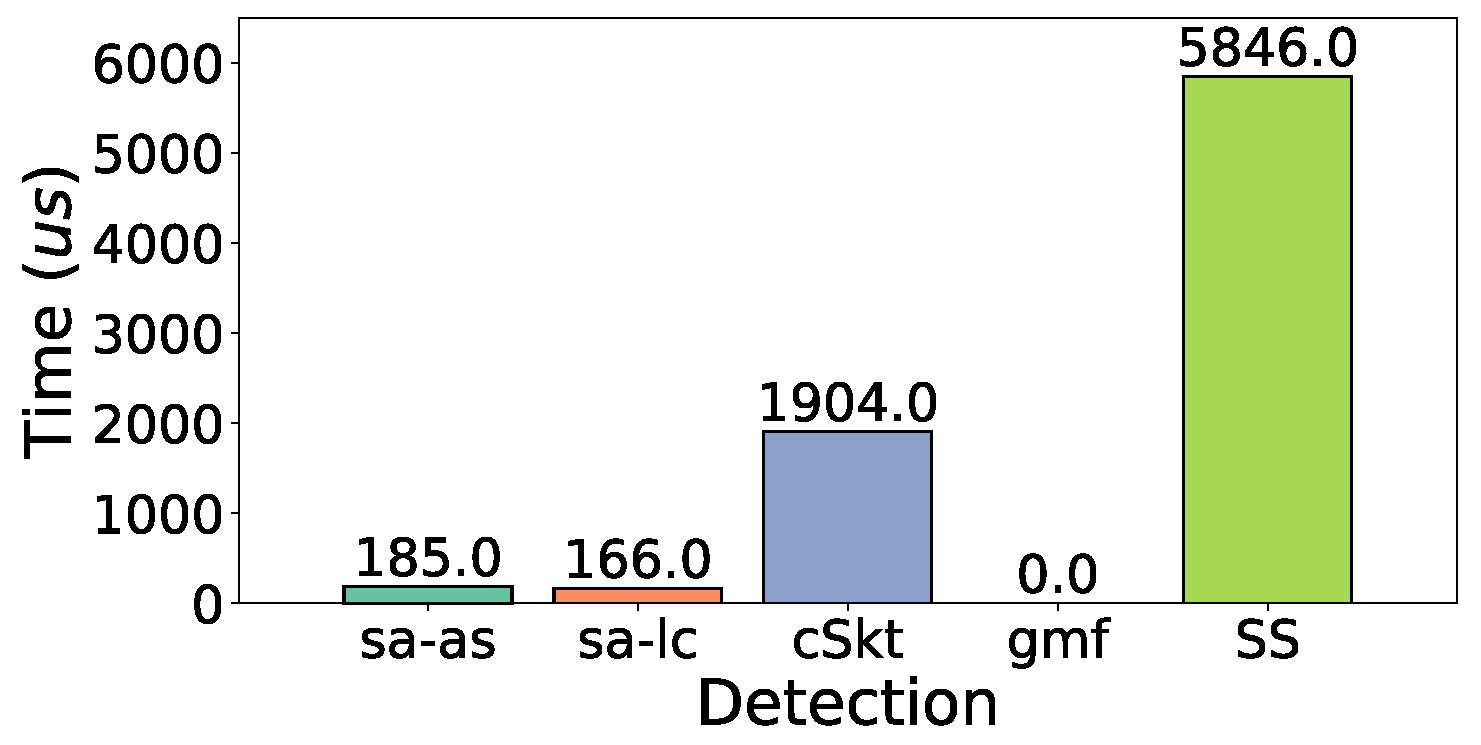
• Detection time: Time spent reporting all super spreads. The experiments were repeated 10 times, and the average detection time was recorded and reported.
• Precision: Fraction of true super spreads reported over all reported spreads.
• Recall: Fraction of true super spreads reported over all true super spreads.
• F1 Score: The F1 score is the harmonic mean of the precision and recall, which is defined as $\frac{2\cdot \mathrm{P}\mathrm{r}\mathrm{e}\mathrm{c}\mathrm{i}\mathrm{s}\mathrm{i}\mathrm{o}\mathrm{n}\cdot \mathrm{R}\mathrm{e}\mathrm{c}\mathrm{a}\mathrm{l}\mathrm{l}}{\mathrm{P}\mathrm{r}\mathrm{e}\mathrm{c}\mathrm{i}\mathrm{s}\mathrm{i}\mathrm{o}\mathrm{n}+\mathrm{R}\mathrm{e}\mathrm{c}\mathrm{a}\mathrm{l}\mathrm{l}}$.
• Average Absolute Error (AAE): AAE is defined as $\frac{1}{\left|\mathsf{\Psi }\right|}\sum _{f_i\in \mathsf{\Psi }}|n_i-\widehat{n_i}|$, where $\mathsf{\Psi }$ is the true super spreads reported.
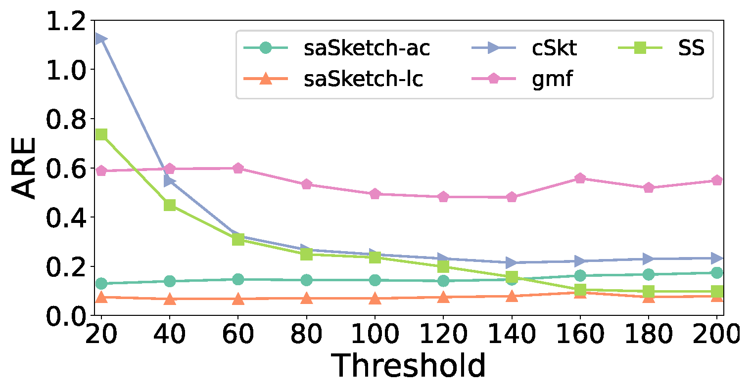
• Average Relative Error (ARE): ARE is defined as $\frac{1}{\left|\mathsf{\Psi }\right|}\sum _{f_i\in \mathsf{\Psi }}\frac{|n_i-\widehat{n_{\mathrm{i}}}|}{n_i}$.

The throughput and detection time were used to measure the insert speed and query speed, reflecting the performance. And the Precision, Recall, and F1 Score were used to measure the accuracy of super spread detection. AAE and ARE were devoted to measuring the error of the cardinality estimation.

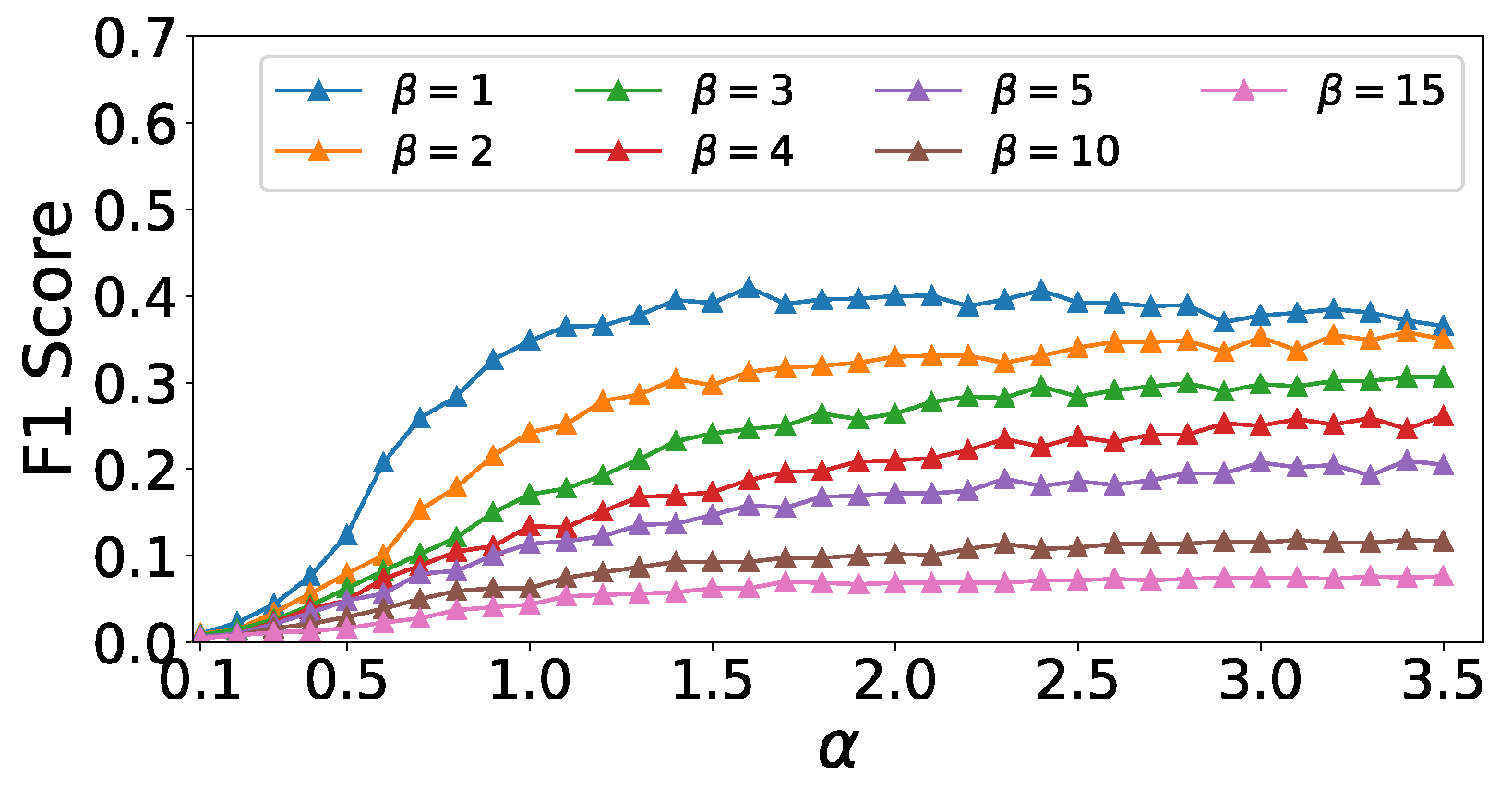
5.3. Experiments on Parameters $\alpha$ and $\beta$

In this section, we conducted several experiments to evaluate the effects of the parameters $\mathsf{\alpha }$ and $\mathsf{\beta }$ on SSD-AIS. In particular, we took saSketch-lc as a representation of SSD-AIS in the e-commerce dataset. Here, we hope to find suitable $\mathsf{\alpha }$ and $\mathsf{\beta }$, rather than the optimal $\mathsf{\alpha }$ and $\mathsf{\beta },$ for a certain dataset or sketch of the saSketch family. In fact, the following experiments have proven that suitable $\mathsf{\alpha }$ and $\mathsf{\beta }$ have excellent performance for different datasets and sketches in the saSketch family.

In this experiment, we set $d$ to 1, threshold $\mathsf{\Phi }$ to 150, and memory to 40 KB. Figure 4 shows the impact of $\mathsf{\alpha }$ and $\mathsf{\beta }$ on the F1 score of the super spread detection. The F1 score of different $\mathsf{\beta }\mathrm{s}$ increases with an increase of $\mathsf{\alpha }$ and then stabilizes. And the F1 Score with $\mathsf{\beta }=1$ is always the highest. Figure 5 shows the impact of $\mathsf{\alpha }$ and $\mathsf{\beta }$ on the throughput of super spread detection. When $\mathsf{\alpha }=1$ and $\mathsf{\alpha }=2$, there is a sudden increase in throughput for all $\mathsf{\beta }$, because the exponent calculation is faster for integers.

In the following experiment, we set $\mathsf{\alpha }$ to 2 and $\mathsf{\beta }$ to 1.

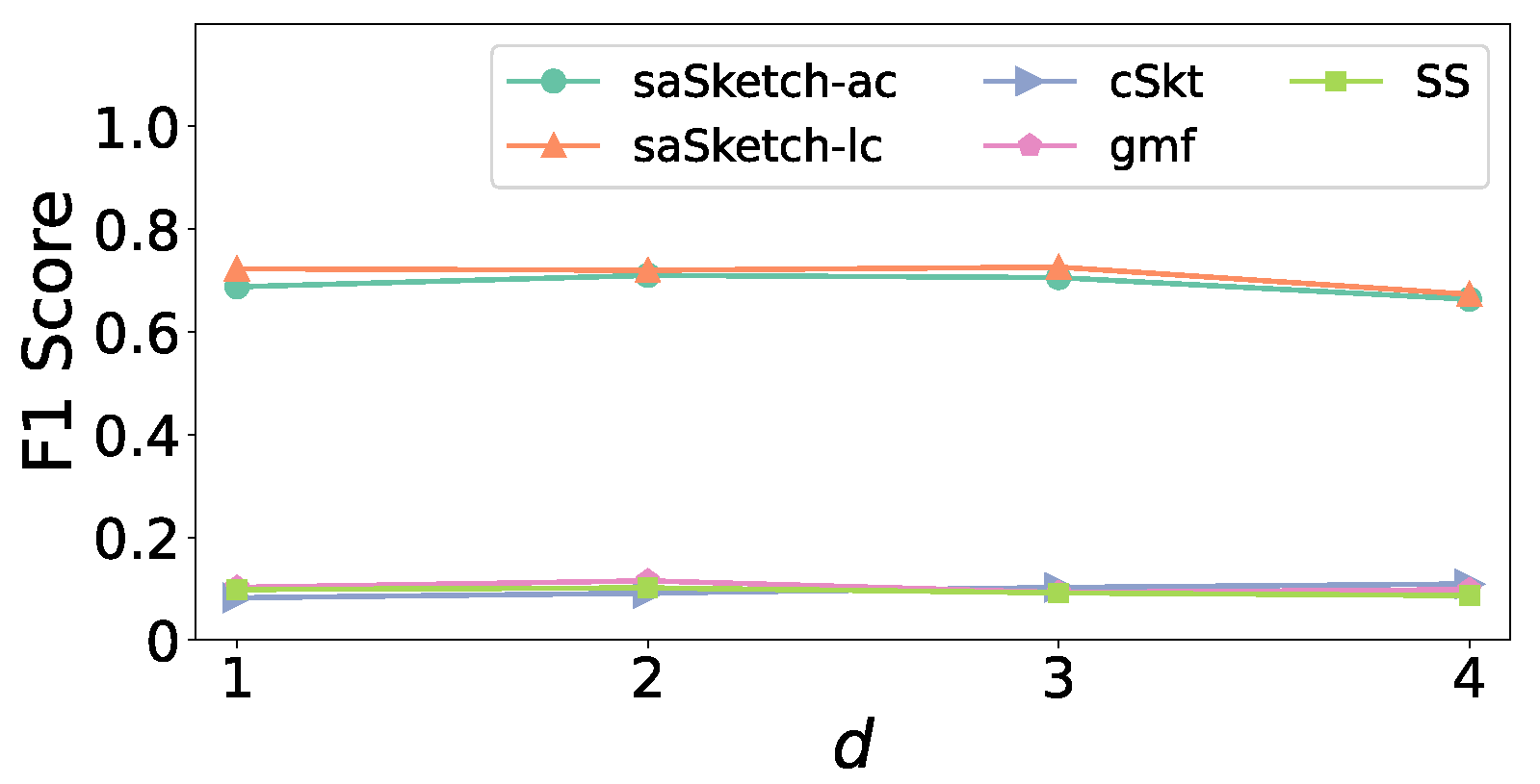
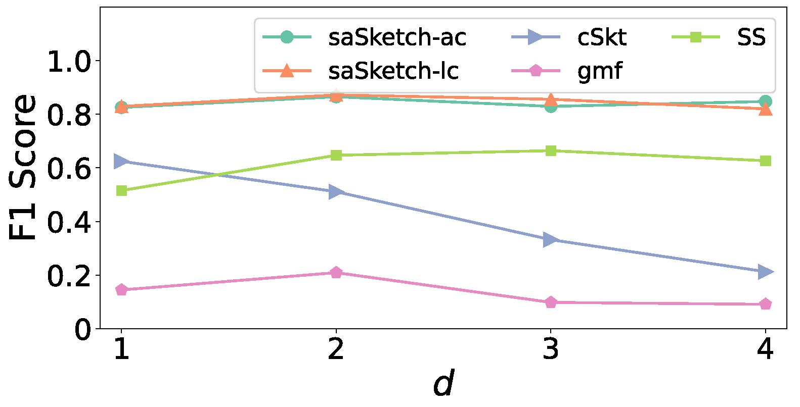
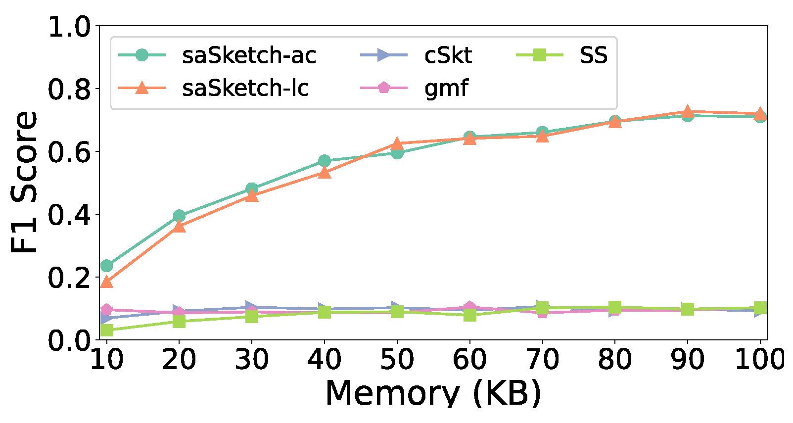
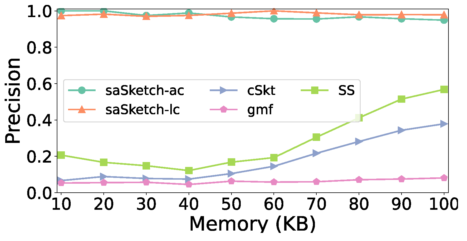
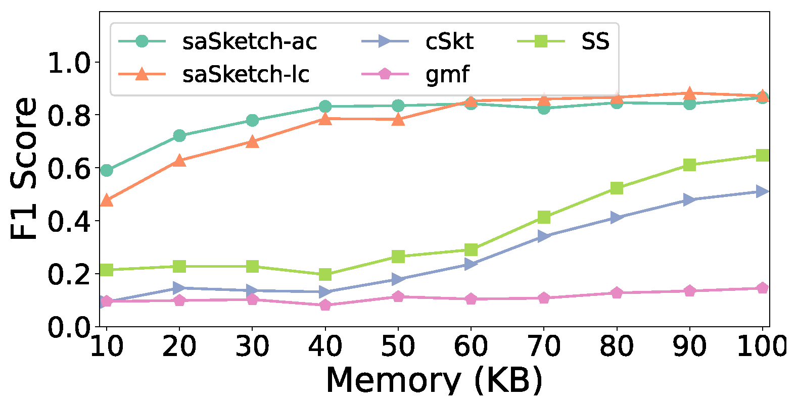
5.4. Experiments on Accuracy

This section used the same array number, memory size, and threshold for each algorithm to obtain a head-to-head comparison for super spread detection. We conducted experiments with various array numbers $d$, memory size, and threshold on the e-commerce datasets and the CAIDA datasets and analyzed the effects of the array number, memory size, and threshold in the above two datasets.

(1)

Effects of $d$

In this experiment, the memory size was equally set to 100 KB for both datasets. We took 5% of the maximum super spread as the threshold, and the thresholds in the e-commerce datasets and CAIDA dataset were about 250 and 100, respectively. The array number $d$ varied from 1 to 4.

Figure 6 and Figure 7 show the impact of $d$ on the F1 score in the e-commerce dataset and CAIDA dataset, respectively. The F1 scores of saSketch-ac and saSketch-lc are always higher than other algorithms for different $ds$. In e-commerce, the F1 scores of saSketch-ac and saSketch-lc are both about 0.73, and 0.12, 0.14, and 0.13 for cSkt, gmf, and SS. Based on the results of the experiments above, we set $d$ to 2 for all algorithms in the following experiment.

(2)

Effect of memory

In this experiment, we took 5% of the maximum super spread as the threshold, then the thresholds in the Recommender System dataset and CAIDA dataset are about 250 and 100, respectively. We set the array number $d$ to 2. In many scenarios, the memory available for flow measurement is very small. For example, the main function of network forwarding equipment is network packet forwarding, so the resources allocated for flow measurement are very small. Thus, the memory size varies from 10 KB to 100 KB.

Figure 8, Figure 9 and Figure 10 show the accuracy of super spread detection in the e-commerce dataset. Figure 8 shows the impact of memory on precision. Changes in memory have little effect on precision. The precision of saSketch-lc and saSketch-ac are significantly higher than the other algorithms. When the memory is set to 50 KB, the precision of saSketch-ac, saSketch-lc, cSkt, SS, and gmf is 0.93, 0.97, 0.06, 0.07, and 0.06, respectively. Note that SS performs well when the memory is large, for example, the precision of SS would reach 0.95 when memory is 5 MB. However, under a small memory, SS cannot contain sufficient nodes, resulting in low precision.

Figure 9 shows the effect of memory on recall. The recall of all algorithms increases as the memory increases. The recall of saSketch-lc and saSketch-ac are both higher than those of the other algorithms when memory is set to larger than 20 KB. When memory is set to 50 KB, the recall of saSketch-ac, saSketch-lc, cSkt, SS, and gmf is 0.44, 0.46, 0.22, 0.12, and 0.15, respectively.

Figure 10 shows the impact of memory on the F1 score. The F1 score of all algorithms increases as memory increases. The F1 scores of saSketch-lc and saSketch-ac are both higher than those of other algorithms with different memories. The F1 score of saSketch-ac, saSketch-lc, cSkt, SS, and gmf is 0.60, 0.63, 0.10, 0.09, and 0.09, respectively, when memory is 50 KB.

Figure 11, Figure 12 and Figure 13 show the accuracy of super spread detection in the CAIDA dataset. The results in the CAIDA dataset are similar to that of the e-commerce dataset except for recall. A small difference in the recall is that cSkt surpasses saSketch-lc and saSketch-ac at 70 KB (Figure 12) and is approximately the same when the memory is larger. The F1 scores of saSketch-lc and saSketch-ac are both higher than those of other algorithms with different memories. The F1 score of saSketch-ac, saSketch-lc, cSkt, SS, and gmf is 0.83, 0.78, 0.18, 0.26, and 0.11, respectively, when the memory is set to 50 KB.

Figure 14 shows the effect of the threshold on the F1 score for the e-commerce dataset. The F1 score of saSketch-lc and saSketch-ac increase as the threshold increases while those of the other algorithms decrease. Figure 15 shows the impact of threshold on the F1 score in the CAIDA dataset. The F1 score of saSketch-lc and saSketch-ac have little change as threshold increases. In conclusion, the F1 score of saSketch-lc and saSketch-ac are both higher than those of the other algorithms with different thresholds.

In conclusion, the F1 scores of saSketch-lc and saSketch-ac are higher than those of the other algorithms with different memories.

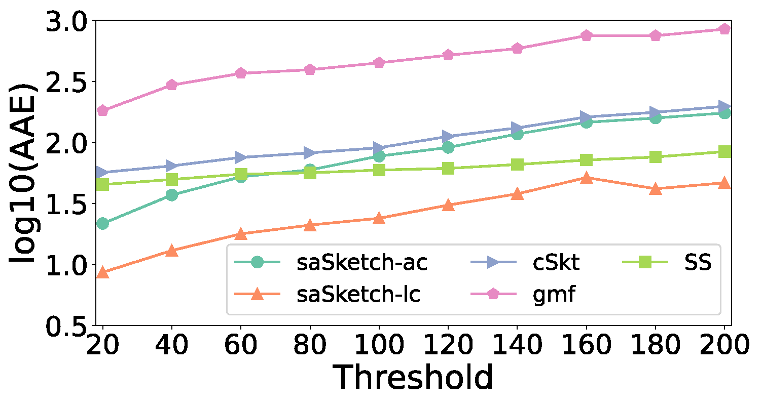
5.5. Experiments on AAE and ARE

In this section, we pay attention to the AAE and ARE of the estimated spread of the reported super spread. We conducted experiments with various memory sizes and thresholds for both datasets. We set the array number $d$ to 2 for all algorithms. Then, we undertook the corresponding analysis.

(1)

Effect of memory

In this experiment, we took 5% of the maximum super spread as the threshold, and the thresholds in the Recommender System dataset and CAIDA dataset are approximately 250 and 100, respectively. The memory size varies from 10 KB to 100 KB.

Figure 16 and Figure 17 show the error of the estimated cardinality of the super spread in the e-commerce dataset. When the memory increases, the AAE and ARE of most algorithms decrease. This is because the number of detected super spreads changes when memory changes.

When memory is 50 KB, the AAE of saSketch-ac, saSketch-lc, cSkt, SS, and gmf is 77, 42, 2163, 4052, and 302 respectively. The ARE of saSketch-ac, saSketch-lc, cSkt, SS, and gmf is 0.15, 0.08, 5.5, 10.5, and 0.41, respectively.

Figure 18 and Figure 19 show the error of the estimated cardinality of the super spread in the CAIDA dataset. The AAE of saSketch-lc is 5.7 times lower than that of cSkt, 4.7 times lower than that of SS, and 23.4 times lower than that of cSkt. The ARE of saSketch-lc is 5.6 times lower than that of cSkt, 7.9 times lower than that of SS, and 68.8 times lower than that of cSkt when the memory is 50 KB.

(2)

Effect of threshold

In this experiment, the memory size was set to 100 KB. The threshold varied from 0.01 to 0.1 of the maximum super spread. In particular, the threshold in the Recommender System dataset varies from 100 to 500 and the threshold in the CAIDA dataset varies from 20 to 200.

Figure 20 and Figure 21 show the error of the estimated cardinality of the super spread in the e-commerce dataset. When the threshold increases, the AAEs of most algorithms increase slightly. When the threshold is 250, the AAE of saSketch-ac, saSketch-lc, cSkt, SS, and gmf is 71, 36, 1012, 1714, and 300 respectively. The ARE of saSketch-ac, saSketch-lc, cSkt, SS, and gmf is 0.15, 0.07, 2.65, 10.5, and 0.41, respectively.

Figure 22 and Figure 23 show the error of the estimated cardinality of the super spread in the CAIDA dataset. The AAE of saSketch-lc is 3.9 times lower than that of cSkt, 2.6 times lower than that of SS, and 19.6 times lower than that of cSkt. The ARE of saSketch-lc is 4.0 times lower than that of cSkt, 3.8 times lower than that of SS, and 8.3 times lower than that of cSkt when the threshold is 100.

5.6. Experiments on Performance

In this section, we focus on the performance of super spread detection. We conducted experiments with varying memory sizes and thresholds on two datasets. We set the array number $d$ to 2 for all algorithms.

Figure 24 and Figure 25 show the insert throughput of adding a flow-element pair of a data stream to a sketch. gmf has the lowest insert throughput because it requires non-negligible time to traverse the flow store structure. SS has the highest throughput as it calculates the length of the longest 0 bit through the hash of the key to update the count value of the bucket, and cSkt, saSketch-ac, and saSketch-lc need to calculate the cardinality estimator after inserting the incoming item into this estimator. saSketch-ac and saSketch-lc are faster than cSkt because the bucket of cSkt has only one cardinality estimator, and each item needs to be inserted into the cardinality estimator to calculate the corresponding value, whereas saSketch-ac and saSketch-lc have two cardinality estimators PEst and NEst per bucket. If the flow label of the incoming item is differentiated from the key of the corresponding bucket, there is a high probability that insertion into the NEst cardinality estimator does not need to be performed. The probability depends on the current pvote value, and the larger the pvote, the higher the probability of ignoring.

Figure 26 and Figure 27 show the detection time of returning all reported super spreads in the e-commerce dataset and CAIDA dataset, respectively. The detection of gmf is 0 because gmf has a structure to store super spreads all the time. SS has the highest detection time because it needs to calculate the spread for traversing each bucket. saSketch-lc and saSketch-ac both return super spreads in a few microseconds.

6. Conclusions

Owing to the limited memory availability, accurately detecting a super spread in heavy data streams faces challenges. Prior algorithms focused more on the accuracy of super spread detection, but could not provide the precise cardinality of a super spread. This paper proposes an innovative sketch called SSD-AIS for super spread detection and corresponding cardinality estimation. Compared with the state-of-the-art work such as SpreadSketch and gmf, the solution we proposed has a higher accuracy in super spread identification under different memory allocations and traffic traces. All related source codes in our work have been released at Github [24].

References

- Tan, L.-Z.; Su, W.; Zhang, W.; Lv, J.; Zhang, Z.; Miao, J.; Liu, X.; Li, N. In-band network telemetry: A survey. Comput. Netw. 2021, 186, 107763. [Google Scholar] [CrossRef]
- Li, S.; Luo, L.; Guo, D. Sketch for Traffic Measurement: Design Optimization Application and Implementation. arXiv 2020, arXiv:2012.07214. Available online: https://arxiv.org/abs/2012.07214 (accessed on 5 January 2021).
- Pendleton, M.; Garcia-Lebron, R.; Cho, J.-H.; Xu, S. A survey on systems security metrics. ACM Comput. Surv. 2017, 49, 62. [Google Scholar] [CrossRef]
- Cao, J.; Jin, Y.; Chen, A.; Bu, T.; Zhang, Z.-L. Identifying high cardinality internet hosts. In Proceedings of the IEEE International Conference on Computer Communications, Rio de Janeiro, Brazil, 19–25 April 2009; pp. 810–818. [Google Scholar] [CrossRef]
- Durumeric, Z.; Bailey, M.; Halderman, J.A. An Internet-Wide View of Internet-Wide Scanning. In Proceedings of the 23rd USENIX Security Symposium, San Diego, CA, USA, 20–22 August 2014; pp. 65–78. Available online: https://www.usenix.org/conference/usenixsecurity14/technical-sessions/presentation/durumeric (accessed on 10 May 2021).
- Fayaz, S.K.; Tobioka, Y.; Sekar, V.; Bailey, M. Bohatei: Flexible and Elastic Ddos Defense. In Proceedings of the 24th USENIX Security Symposium, Washington, DC, USA, 12–14 August 2015; pp. 817–832. Available online: https://www.usenix.org/conference/usenixsecurity15/technical-sessions/presentation/fayaz (accessed on 20 January 2021).
- Liu, Y.; Chen, W.; Guan, Y. Identifying high-cardinality hosts from network-wide traffic measurements. IEEE Trans. Dependable Secur. Comput. 2016, 13, 547–558. [Google Scholar] [CrossRef]
- Qun, H.; Lee, P.P.C.; Bao, Y. Sketchlearn: Relieving user burdens in approximate measurement with automated statistical inference. In Proceedings of the 2018 Conference of the ACM Special Interest Group on Data Communication, Budapest, Hungary, 20–25 August 2018; pp. 576–590. [Google Scholar] [CrossRef]
- Lu, J.; Chen, H.; Sun, P.; Hu, T.; Zhang, Z. OrderSketch: An unbiased and fast sketch for frequency estimation of data streams. Comput. Netw. 2021, 201, 108563. [Google Scholar] [CrossRef]
- Liu, Z.; Manousis, A.; Vorsanger, G.; Sekar, V.; Braverman, V. One sketch to rule them all: Rethinking network flow monitoring with univmon. In Proceedings of the Annual Conference of the ACM Special Interest Group, Florianopolis, Brazil, 22–26 August 2016; pp. 101–114. [Google Scholar] [CrossRef]
- Yang, T.; Jiang, J.; Liu, P.; Huang, Q.; Gong, J.; Zhou, Y.; Miao, R.; Li, X.; Uhlig, S. Elastic sketch: Adaptive and fast network-wide measurements. In Proceedings of the 2018 Conference of the ACM Special Interest Group on Data Communication, Budapest, Hungary, 20–25 August 2018; pp. 561–575. [Google Scholar] [CrossRef]
- Wu, K.; Otoo, E.J.; Shoshani, A. Optimizing bitmap indices with efficient compression. ACM Trans. Database Syst. 2006, 31, 1–38. [Google Scholar] [CrossRef]
- Whang, K.-Y.; Vander-Zanden, B.T.; Taylor, H.M. A linear-time probabilistic counting algorithm for database applications. ACM Trans. Database Syst. 1990, 15, 208–229. [Google Scholar] [CrossRef]
- Durand, M.; Flajolet, P. Loglog counting of large cardinalities. In Proceedings of the Algorithms-ESA 2003: 11th Annual European Symposium, Budapest, Hungary, 16–19 September 2003; pp. 16–19. [Google Scholar]
- Cai, M.; Pan, J.; Kwok, Y.-K.; Hwang, K. Fast and accurate traffic matrix measurement using adaptive cardinality counting. In Proceedings of the Annual Conference of the ACM Special Interest Group on Data Communication Workshop on Mining NETWORK Data, Philadelphia, PA, USA, 26 August 2005; pp. 205–206. [Google Scholar] [CrossRef]
- Flajolet, P.; Fusy, É.; Gandouet, O.; Meunier, F. Hyperloglog: The Analysis of a Near-Optimal Cardinality Estimation Algorithm. In Proceedings of the Discrete Mathematics and Theoretical Computer Science, Nancy, France, 1 January 2007; pp. 127–146. Available online: https://algo.inria.fr/flajolet/Publications/FlFuGaMe07.pdf (accessed on 5 December 2020).
- Zhang, Z.; Hsu, C.; Au, M.H.; Harn, L.; Cui, J.; Xia, Z.; Zhao, Z. PRLAP-IoD: A PUF-based Robust and Lightweight Authentication Protocol for Internet of Drones. Comput. Netw. 2024, 238, 110118. [Google Scholar] [CrossRef]
- Cormode, G.; Muthukrishnan, S. Space efficient mining of multigraph streams. In Proceedings of the Twenty-Fourth ACM SIGACT-SIGMOD-SIGART Symposium on Principles of Database Systems, Baltimore, MD, USA, 13–15 June 2005; pp. 271–282. [Google Scholar] [CrossRef]
- Ma, C.; Chen, S.; Zhang, Y.; Xiao, Q.; Odegbile, O.O. Super spreader identification using geometric-min filter. IEEE/ACM Trans. Netw. 2022, 30, 299–312. [Google Scholar] [CrossRef]
- Tang, L.; Huang, Q.; Lee, P.P.C. SpreadSketch: Toward Invertible and Network-Wide Detection of Superspreaders. In Proceedings of the IEEE INFOCOM 2020-IEEE Conference on Computer Communications, Toronto, ON, Canada, 6–9 July 2020; pp. 1608–1617. [Google Scholar] [CrossRef]
- Venkataraman, S.; Song, D.X.; Gibbons, P.B.; Blum, A. New Streaming Algorithms for Fast Detection of Superspreaders. In Proceedings of the Network and Distributed System Security Symposium, San Diego, CA, USA, 2 February 2005; Available online: https://www.ndss-symposium.org/ndss2005/new-streaming-algorithms-fast-detection-superspreaders/ (accessed on 17 March 2021).
- Estan, C.; Varghese, G.; Fisk, M. Bitmap algorithms for counting active flows on high speed links. IEEE/ACM Trans. Netw. 2003, 14, 925–937. [Google Scholar]
- Boyer, R.S.; Moore, J.S. MJRTY: A Fast Majority Vote Algorithm. Autom. Reason. Essays Honor. Woody Bledsoe 1991, 1, 105–118. [Google Scholar]
- SuperKeeper. Available online: https://anonymous.4open.science/r/SuperKeeper-B004/README.md (accessed on 15 March 2021).
- Liu, Y.; Chen, W.; Guan, Y. A fast sketch for aggregate queries over high-speed network traffic. In Proceedings of the IEEE International Conference on Computer Communications, Orlando, FL, USA, 25–30 March 2012; pp. 2741–2745. [Google Scholar] [CrossRef]
- Wang, P.; Guan, X.; Qin, T.; Huang, Q. A data streaming method for monitoring host connection degrees of high-speed links. IEEE Trans. Inf. Forensics Secur. 2011, 6, 1086–1098. [Google Scholar] [CrossRef]
- Liu, W.; Qu, W.; Gong, J.; Li, K. Detection of superpoints using a vector bloom filter. IEEE Trans. Inf. Forensics Secur. 2016, 11, 514–527. [Google Scholar] [CrossRef]
- Zhou, Y.; Zhang, Y.; Ma, C.; Chen, S.; Odegbile, O. Generalized sketch families for network traffic measurement. ACM Meas. Anal. Comput. Syst. 2019, 3, 1–34. [Google Scholar] [CrossRef]
- Cormode, G.; Muthukrishnan, S. An improved data stream summary: The count-min sketch and its applications. J. Algorithms 2005, 55, 58–75. [Google Scholar] [CrossRef]
- Yu, M.; Jose, L.; Miao, R. Software Defined Traffic Measurement with OpenSketch. In Proceedings of the 10th USENIX Symposium on Networked Systems Design and Implementation, Lombard, IL, USA, 2–5 April 2013; pp. 29–42. Available online: https://www.usenix.org/conference/nsdi13/technical-sessions/presentation/yu (accessed on 15 January 2021).
- Schweller, R.T.; Li, Z.; Chen, Y.; Gao, Y.; Gupta, A.; Zhang, Y.; Dinda, P.A.; Kao, M.-Y.; Memik, G. Reversible sketches: Enabling monitoring and analysis over high-speed data streams. IEEE/ACM Trans. Netw. 2007, 15, 1059–1072. [Google Scholar]
- Ecommerce Dataset. Available online: https://www.kaggle.com/retailrocket/ecommerce-dataset?select=events.csv (accessed on 15 January 2021).
- The Caida Anonymized Internet Traces. 2016. Available online: http://www.caida.org/data/overview/ (accessed on 17 March 2021).
- Murmurhash. Available online: https://github.com/aappleby/smhasher/tree/master/src (accessed on 15 June 2021).