Abstract
Due to the long-term exposure of bridge ties to complex environments, their internal steel wires are prone to corrosion damage, which may lead to tie breakage accidents if not detected in time. Although existing advanced monitoring methods can be used to obtain the broken wire signal, they either still need the damage to be identified manually or are limited by the training data set. To address this problem, a model combination consisting of a classification model and three regression models was built based on convolutional neural networks to predict the location of broken wires after first classifying them based on features. We developed software-containing data set generation and model performance testing functions, in which we used original algorithms to expand the broken wire data set for training based on the measured data obtained from FBG sensors with a sampling frequency of 100 Hz, thus generating more than 22,000 types of data. The performance test results showed that the model combination successfully detected 11,972 broken wires among 12,000 test data points generated by the algorithm, with a recognition success rate of 99.77% and an average time of 0.0076 s between the predicted location and the actual broken wire location, with an error rate of 0.38%. In the test of 118 real broken wires, the model detected all the abnormalities, and the average time between the predicted location and the actual broken wire location was 0.0695 s, with an error of 3.48%. This verified the feasibility of using artificial intelligence to accurately identify broken wire signals and can provide a reference for the subsequent intelligent identification of tie abnormalities.
1. Introduction
As the lifeline of cable-stayed bridges, the bracing cable plays the role of linking and supporting the bridge deck’s main girders and towers, and its internal steel strand is the main load-bearing member. Due to the long-term exposure of cable-stayed bridges to the complex natural environment, the steel strand will inevitably produce rust and undergo corrosion, which will lead to wire breakage [], and if not detected and dealt with in time, this will then lead to more serious safety accidents [,]. Therefore, an effective monitoring method is needed to detect broken wires so as to take relevant measures in time to avoid the occurrence of bridge safety problems and accidents.
The main current methods used for broken wire detection are the pressure sensor method, magnetic detection method, digital image method, acoustic emission method, and FBG sensor method. The pressure sensor method is mainly used to estimate the state of the wire inside the ties through the measurement of the cable force [], which is more limited. The basic principle of the magnetic detection method is to determine whether the bracing cable is broken based on the change in the magnetic flux of the magnetized metal [,], and Zhang et al. [] conducted multidimensional self-leakage magnetic detection experiments for different wire breakage states of parallel wire bundles and proposed a method to quantitatively characterize the axial wire breakage width of the bracing cable using a Boltzmann fitting curve. However, this method is susceptible to electromagnetic interference, and the magnetic poles are susceptible to chemical corrosion, leading to magnetic flux leakage. Du et al. [] used a digital image-based detection method to identify abnormalities in the ties via image special point capture, but this method is less stable and is susceptible to environmental factors such as wind, temperature, and humidity. Xin [] proposed a method to discriminate wire break acoustic emission based on signal time domain waveforms, and Yu et al. [] produced a self-aware steel strand with an embedded fiber Bragg grating (FBG) strain sensor pre-compressed to the center wire of the strand. Although both the acoustic emission method and the FBG sensor method can accurately observe the broken wire signal, they still require manual judgment of the identified signal.
In recent years, with the improvement of the arithmetic level of chips, the application field of machine learning has been expanded, and its applications in medical, engineering, and financial fields have become focal points of research []. Artificial neural network algorithms can fully approximate arbitrarily complex, nonlinear relationships due to their excellent self-adaptive, self-organizing, and self-learning capabilities [,]. Attempts have been made to free the identification of bracing cable anomalies from manual constraints using artificial neural network algorithms. Yan et al. [] used a basic BP neural network to predict the effect of the bridge overload problem on the bracing cable state and adjusted the weights of neurons using the L-M optimization algorithm after each calculation. The estimation error of the final model was 0.352%. However, BP neural network is a local search optimization method [], and the algorithm is prone to falling into local extremes [] and overfitting, leading to model training failure, and it requires manual feature selection. Moreover, it is difficult to choose the appropriate features; thus, BP neural networks are now being replaced by more advanced models. Feng et al. [] in order to obtain a model for studying corrosion, used BP, RBF, and LS-SVM for the prediction. The prediction accuracy of LS-SVM was significantly higher than that of the other two models, which also confirmed the performance deficiencies of BP neural networks, although SVM involves the operation of an m-order matrix in the calculation, which makes it difficult to implement using large-scale training samples. CNN convolutional neural networks are a class of feedforward neural networks that include convolutional operations, which achieve the encapsulation of feature extraction and avoid the explicit extraction of features [,], thus perfectly solving the shortcomings of BP neural networks. Park et al. [] built a regression model using convolutional neural networks in order to extract information that can be used to identify the location of the bracing cable damage from the measured acceleration response, but their study was limited by the training data. Zhang et al. [] attempted to generate dummy data using GAN adversarial neural networks for training purposes, but the reliability of the model could not be demonstrated, as it could easily lock in a single pattern for generation during GAN data generation, and it required the conversion of the leakage signal into a time–frequency image in order to perform the calculation, which was computationally intensive. In fact, convolutional neural networks have achieved extremely high accuracy in pure signal processing, such as the recognition of seismic wave signals [], radar signals [], etc.
In summary, for bridge cable breakage anomalies, the FBG sensor method and acoustic emission method can obtain the broken wire signal with sufficient accuracy but need the break to be identified manually. Although the intelligent identification of the signal is currently achieved based on the convolutional neural network and magnetic detection method, the performance is limited by the training data set and needs to be improved. According to similar demands, CNN (convolutional neural network) can meet the demand of identifying signal data with high accuracy if the training data set meets the requirements. This study intended to address internal wire breakage anomalies of bridge ties using the natural environment in which the bridge is located as the research context. First, tensioning experiments were conducted to collect wavelength signal data using FBG sensors, and algorithms were written to expand the data set. Then, a combination of convolutional neural network models was built for calculation to achieve the high-accuracy automatic identification of broken wires.
2. Basic Theory of One-Dimensional Convolutional Neural Networks
The convolutional neural network originated from the field of computer vision, and its main structure includes an input layer, convolutional layer, pooling layer, fully connected layer, and output layer. The input layer is used to input information, the convolutional layer is used to extract the underlying features of the information, the pooling layer can prevent overfitting and reduce the dimensions of the data, the fully connected layer is used to summarize the feature information obtained from the convolutional layer and the pooling layer, and the output layer obtains the result based on the information from the fully connected layer. Extending the theory to one-dimensional reality, the process is much the same. Let us take a one-dimensional tensor I of length 5 and a convolutional sum K of length 3 as an example. In the convolution process, K moves along I, and each time it moves to a fixed position, the values at the corresponding positions are multiplied and then summed. The calculation process is shown in Figure 1.
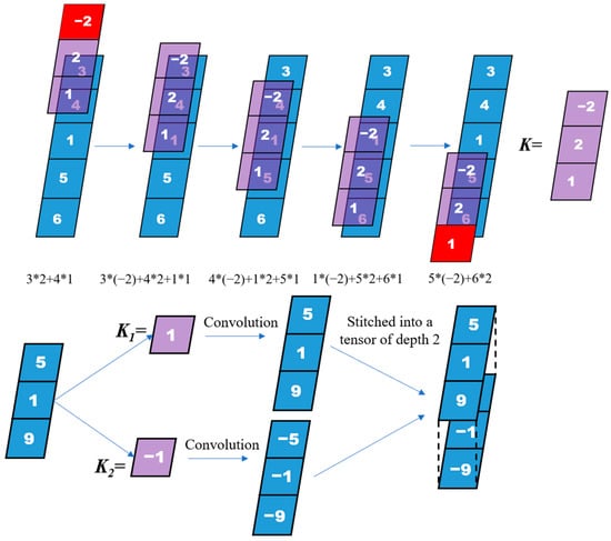
Figure 1.
One-dimensional convolution calculation process. *: Multiplication operations.
There are three methods of convolution. In this calculation process, the principle is more or less the same as in full convolution and valid convolution, but the starting point and end point of the calculation of the convolution and tensor are different. In the actual calculation, there is more than one convolutional sum. Supposing that there are n convolutional sums, after the completion of the calculation, one can obtain the depth of n tensor.
The optimizer can identify the parameters that allow the loss function to be minimized. This model uses the Adam optimizer, which can correlate the gradients of all the samples, thus facilitating the solution of the global optimal solution, and always contains the information of the previous gradients, enabling gradient conduction [], with the following principal Formula (1):
For the regression models, the activation function generally uses relu, with the expression (2):
For the classification model, the activation function is generally Softmax, and the expression is (3):
In the formula, zi is the output value of the ith node, and C is the number of output nodes, that is, the number of categories of classification. With this function, the output values of multiple classifications can be converted into probability distributions ranging from [0, 1] to 1 so as to achieve the classification.
CNN avoids the extraction of explicit features and implicitly learns from training data. Because the weights of neurons on the same feature mapping surface are the same, the network can learn in parallel, which is a major advantage of CNN compared with the fully connected neural network. The specific structure of CNN local weight sharing gives it unique advantages in speech recognition, image processing, and signal recognition.
3. Tension Experiment
Due to the advantages of fast transmission speed, good durability and low cost, fiber Bragg Grating (FBG) is widely used in the field of information and electronic data transmission. The main principal is as follows: As the grating can screen the incident light, the screened incident light will be reflected back through the circulator into the demodulator instrument; as the demodulator measures the change in wavelength, after conversion, we can obtain the physical quantities we need.
In order to obtain the basic data of the characteristic signal of the broken wire, a tensile test based on the FBG strain sensor was conducted. A 1 mm deep and 1 mm wide groove was created in the center wire of the strand, and the FBG sensor was placed in the groove to prepare the smart center wire. Then, the smart center wire and the side wire were twisted into a self-perceiving strand. A total of 57 bundles of ordinary low-relaxation prestressing strands with a length of 5 m were taken for the test, and they were divided into three groups. Each group consisted of 19 bundles of strands, and in each group, specimen A was a self-perceiving strand, and specimens Bij, Cij, and Dij were the common single-side wire damage area for the steel strands and the damage location as the parameters of change. Figure 2a,b shows the side wire damage schematic diagram, and the specific parameters are shown in Table 1. The distribution of the steel strand on the anchor plate is shown in Figure 2c, and the tensioning machine used in the test is shown in Figure 2d. During the test, the tensioning machine was loaded slowly at a uniform speed until all the defective wires broke, as shown in Figure 2e, and the data were collected in real time using a demodulator connected to the self-aware steel strand at a frequency of 100 times per second.
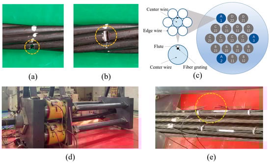
Figure 2.
(a,b) Damage area of single strand of B11 steel strand 2/3. (c) Distribution of steel strands on the anchorage plate. (d) Physical drawing of the pretest tensioning machine. (e) Steel strand after wire breakage.

Table 1.
Edge wire damage of each group of specimens.
The wavelength data obtained from the A1, A2, and A3 self-aware strands were recorded for each common strand break, and a total of 144 wire break data points were obtained after the three sets of tests were completed. However, some of the data showed a sudden drop in the image wavelength change value at the moment of the wire break signal detected by the self-aware steel strand during the rise, which is most likely due to the uneven force on the wire in the drawstring. The frequency of the single wire’s vibration propagated to the vibration of the anchor end at the moment of the hairline break, resulting in unsynchronized vibration between some of the strands at the moment of the drawstring’s break. Such data were identified as invalid features, as shown in Figure 3a,b.
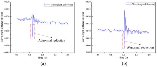
Figure 3.
Invalid feature data (abnormal wavelength reduction), (a,b) show the characteristics of the two anomalous data.
Finally, the invalid feature data were removed, and 118 valid wire breakage feature data points were collated. Due to the different locations of the self-perceived strands, as well as the locations of the tie damage and the damage area, the data showed three different characteristics of wire break signals, and all the wire break signals appeared based on these three characteristics. Only the amplitude of the wavelength signal vibration and the time point of the appearance of the wire break differed. Based on the data collected in this experiment, the algorithm was written to simulate the filament break data in order to expand the training data set. Additionally, we built a neural network model for signal recognition.
4. Data Set Preparation
The reliability and quantity of the data set directly determine the training limit of the model. In order to obtain a high-performance model, the wire break data measured in the test were divided into three categories according to their curve shape characteristics, and one data point with complete characteristics and a balanced amplitude was taken as the base data point for each of these three categories. The algorithm was written in such a way that the location and amplitude of the wire break would randomly change so as to obtain completely different wire break data, which were then generated in batches and used for the training of the neural network model. The specific data generation process and the base data are shown in Figure 4.
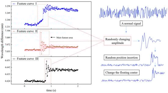
Figure 4.
Three sets of original data and main logic of broken wire data generation algorithm.
The method of data generation in the debugging phase is encapsulated in the node.js backend code, which can be called by sending a request when required by the frontend. First, a section of normal data with a length of 200 must be generated according to the corresponding normal data float range. Here, for the convenience of graphing and calculation, the base value of the wavelength difference is changed to 0, only the number after the 10th digit is retained, and the shape is kept intact without affecting the feature extraction. Here, we chose to use the two-dimensional array directly (including the coordinate axis) and redefine each sub-element of the generated array as an array. In this way, when the loop is used to assign the array, it is necessary to judge whether it is the coordinate value or the wavelength difference. Here, Y represents the generated wavelength difference in nm, R represents the random number ranging from 0 to 1, and max and min represent the maximum and minimum values of the generated data:
Here, i is used to represent the number of cycles, and X represents the value of the coordinate axis in s:
The anomaly part can be defined as follows: Firstly, one needs to randomly select one of the three feature data points as the base data point, and as each group of feature data has a different length, the length needs to be recorded. Then, one defines the location where the anomaly starts and the amplitude of the curve. The specific settings of the three features are different, and the specific parameters are shown in Table 2.
Table 2.
The relevant parameters of the three features.
Here, the map method is used to multiply each item in the array according to the amplitude. In order to achieve the tensile effect of the curve and simulate the change in the vibration amplitude of the signal, it is necessary to specifically process the points below the floating center. Here, F represents the center of the floating curve, and A represents the randomly generated amplitude:
After the exception fragment is generated, the generated exception fragment needs to be inserted into the specified position of the curve according to the previously defined start position. One first locates the insertion position through the loop and then uses the data of the exception fragment array to replace the data of the specified length after the insertion position. Here, we must consider that when the start position is excessively backward and the length is not sufficient to insert the whole exception fragment, special treatment should be applied. When the sequence number is greater than or equal to 201, one must use a break to jump out of the loop. After the insertion of the abnormal data is completed, the floating center of the signal needs to be changed according to the amplitude. Here, we chose to multiply the corresponding data change range directly with the amplitude and then replace the data in the corresponding position of the array. If the length is not sufficient to insert the entire exception fragment, this step is not required.
Finally, the final generated array needs to be processed to retain a four-digit decimal number. In order to test the model using real data, a specific method is developed, and calling this method will directly return a segment of real broken wire data with a length of 200 for the testing of the model. At this point, the backend work is completed, and the generated exception data are returned to the frontend. The main logic of this process, on the software level, is shown in Figure 5.
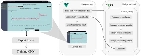
Figure 5.
The working process of the software (to generate broken wire data).
The frontend of the software is built based on the advanced framework Vue, which is a single-page application. When the frontend turns on the Get Data button, an ajax request is sent, and the backend returns a data point with a length of 200. To facilitate the debugging of the code and observation of the data generation effect, the frontend introduces ECharts for data plotting, which is an open-source visualization library implemented in JavaScript that relies on the vector graphics library ZRender []. It provides intuitive, interaction-rich, and highly customizable data visualization charts.
Figure 6 shows a screenshot of the software, demonstrating the four types of broken filament data generated by the algorithm with different amplitudes and start positions (Figure 6c is the same as Figure 6d regarding the feature type). After rendering, if one needs to view the specific data, one can choose to export the data to a csv format file. The derivation method is string splicing, separating each data point with a comma and splicing the starting position of the broken filaments in the last column to facilitate the training of the neural network model.
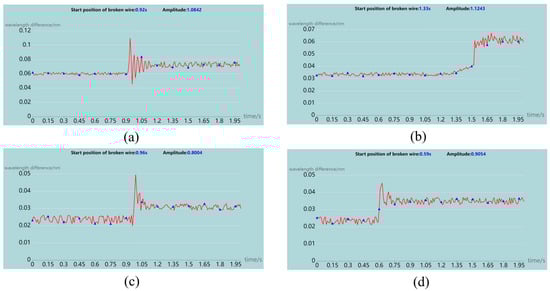
Figure 6.
Software generates wire breaking data group diagram. (a) Start position = 0.92 s, amplitude = 1.0842, feature type = 1. (b) Start position = 1.33 s, amplitude = 1.1243, feature type = 2. (c) Start position = 0.96 s, amplitude = 0.8004, feature type = 0. (d) Start position = 0.59 s, amplitude = 0.9054, feature type = 0.
The above is the process of generating, graphing, and exporting a single data point. After familiarizing ourselves with this process, we prepared the batch export function, which is the core function of the data set. This function has two types of batch generation modes. These are specified feature anomaly data generation and classification pattern data generation, respectively. In order to handle the performance requirements of large-batch data generation, we copied the data generation method to the frontend to avoid communication problems and to facilitate the creation of multiple calls in a short period of time. For the classification pattern data generation channel, instead of splicing the filament break start time, the feature type was spliced in the last column. Regarding the generation speed of this algorithm, for this computer (the CPU is Intel core i5-13600 kf), the generation of 30,000 anomalous data points only takes approximately 8.5 s, and the algorithm’s performance meets the requirements for the experiment, which provides reliable data support for the training of the neural networks.
5. Model Construction
The environment used to build the model in this study was Python 3.8.5. We used the tensorflow machine learning framework, and the encoder was vscode. The computation process of the model combination is shown in Figure 7. The classification model first determines whether there is a broken wire and the type of feature that appears. If a break is detected, the corresponding regression model is called to calculate the location of the broken wire. The regression model contains four convolutional layers, four pooling layers, and four fully connected layers. The activation function uses relu, the optimizer uses Adam, and the pooling layer is set to use the average value for pooling. The specific model structure is shown in Figure 8. The classification model’s structure is approximately the same, and the activation function of the last layer is changed to Softmax.
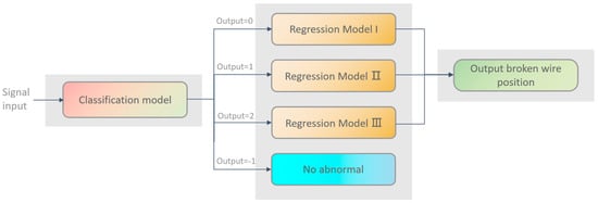
Figure 7.
Model combination calculation process.
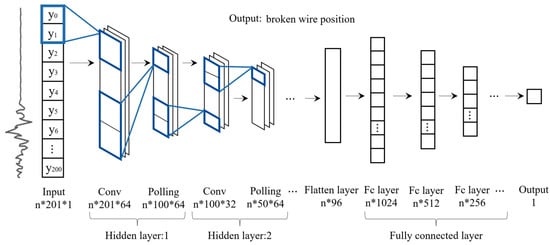
Figure 8.
Neural network architectures. *: Multiplication operations.
The loss function for the categorical model was chosen to be sparse categorical crossentropy, while for the three regression models, we conducted a performance comparison of two loss functions, MAE (mean absolute error) and MSE (mean squared error), which are calculated as follows:
The epoch was fixed at 100 times throughout the test. The average error, an index for evaluating the performance of the model, was introduced. The error is the difference between the starting position of the broken wire and the actual position calculated by the regression model after the classification model has judged the anomaly. N represents the number of batch test data points, and the batch test function of the software was used here. This function is described in detail below, in the Test section (Section 6) of this article. Here, T represents the real location of the broken wire, and t represents the calculation result of the model. The average error (unit is s) is calculated as:
The training data set is 30,000 points of broken wire data possessing specific features generated by the algorithm, with a length of 200 and a simulation time length of 2 s. The test data set is generated in the same way, with a number of 1200. After each epoch, the model is saved in json format. The changes in the loss function and the mean error of the three regression models that occurred with the increase in the epoch are shown in Figure 9, Figure 10 and Figure 11.
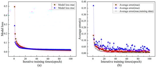
Figure 9.
The loss (a) and average error (b) of the model change with the increase in the epoch (feature No. 1).
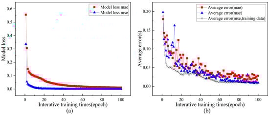
Figure 10.
The loss (a) and average error (b) of the model change with the increase in the epoch (feature No. 2).
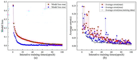
Figure 11.
The loss (a) and average error (b) of the model change with the increase in the epoch (feature No. 3).
For the first feature, from the loss image, we can see that the MAE loss function converges slightly slower than the MSE loss function, but the final convergence value is lower, which matches the average error image. The average error of the MAE loss function decreases in a relatively steady manner, and the final error is lower. For the second feature, from the loss image, we can see that the MSE loss function converges not only faster but also to a lower value, and from the average error image, we can see that the MSE loss function does render the error lower compared to the MAE loss function. For the third feature, the situation is very similar to that of feature 2, but the stability of the two functions in the average error image is less than that of the first two features.
Taken together, the average error metric proposed in this study has the same basic change trend as the loss. For both the MAE and MSE error functions, their performance varies according to the training features, and the process of decreasing the average error is less stable, because feature 3 is slightly more difficult to identify compared to the first two features. Finally, for feature 1, MAE is chosen as the error function, and for features 2 and 3, MSE is chosen as the error function, and all three functions converge to below 0.022.
For the selection of the model learning rate, due to the limitation of the arithmetic equipment, only 10 learning rates between 1 × 10⁻⁴ and 0.001, with 1 × 10⁻⁴ as the gradient, were explored in this study when the epoch was fixed to 100. It was found that model 3 could converge to the optimal value when the learning rate was 4 × 10⁻⁴, while models 1 and 2 did not significantly converge to the optimal value in this interval. The model learning rate was chosen to be the value with the lowest average error in the experiment. The specific experimental data are shown in Figure 12a.
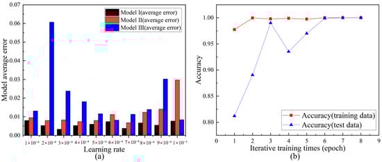
Figure 12.
(a) The influences of different learning rates on three regression models. (b) Classification model accuracy changes with the epoch.
For the classification model, the training data used formed a data set of 30,000 abnormal data points together with 10,000 normal data points, and the test data formed a data set of 1200 abnormal data points together with 200 normal data points. In this case, the algorithm no longer stores the starting position of the broken wire in the last column, and the classification of the storage model is −1, 0, 1, 2. When the model cannot detect abnormalities, it will output negative numbers. When the model determines the anomaly, the corresponding regression model is called to calculate the location of the broken wire. When training to the sixth epoch, the accuracy of the model reaches 100%. The specific image is shown in Figure 12b.
6. Test
In order to facilitate the performance testing of the model, the testing module of the software was written. After finishing the training of the model, we used the tensorflow.js plugin to save the model in json format and the model weights in bin format so that we could obtain a complete model by reading these two files using the web-side software. The web-side software requires one to import the tensorflow.js plugin, and the await asynchronous method is used to read the model files. After the model has been read, one can choose a single data test, as shown in Figure 13, or one can choose a batch data test. For the batch test, one can specify the composition of the batch test data set (the number of abnormal data points and normal data points), and the software will count the number and proportion of abnormal data points detected by the model and calculate the average error between the model judgment position and the real broken wire position.
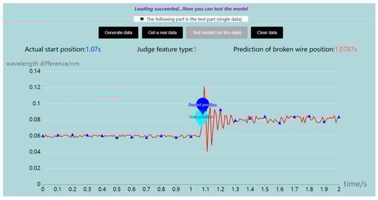
Figure 13.
A single data test diagram (the deep blue point in the diagram is the model calculation result, and the other color is the actual value).
In order to test the model using real data, a special data channel was prepared, and when data were acquired through this channel, the software read the real data set stored in the backend. This real data set comprised 118 effective broken wire data points obtained in the tension experiment.
7. Interference Experiment
In order to verify whether the model can identify the broken wire signal from other anomalous signals, we designed interference experiments. We used an algorithm similar to the one used to generate the broken wire signal, adding pulsed and stepped signals of random amplitude to the normal signal sequence. It is worth mentioning that both pulse and step signals have positive and negative values, and we choose to randomly determine their positive and negative values in the generation algorithm. The generation process is shown in Figure 14.
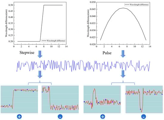
Figure 14.
Generation of step and pulse anomaly signals (The blue line represents a normal segment of the signal, and the red line is the signal after an abnormality has been added).
The final test data set we selected was 7000 pulse anomalies plus 7000 step anomalies, superadd 7000 broken wire anomalies, totaling 21,000 data. The final results are as follows: among the 7000 pulse anomalies, 6803 data have a calculated result of −1, i.e., non-broken wire anomaly, with an accuracy rate of 97.19%; among the 7000 step anomalies, 6911 data have a calculated result of −1, with an accuracy rate of 98.73; among the 7000 broken wire anomalies, there are 6983 positive numbers in the calculation, which is 99.76% correct without considering the classification results. In summary, among 21,000 data, 20,697 data have correct calculation results, and the accuracy rate is 98.56%.
8. Results
After the final model was trained, the software batch test function was used to generate a test data set consisting of 12,000 abnormal data points and 2000 normal data points. Among the 12,000 abnormal data points, the classification model judged 11,972 abnormalities. The correct classification rate for the judged abnormalities was 100%, and the model accuracy rate was 99.77%. For these 11,972 abnormal data points, the absolute error between the filament break position calculated by the regression model and the actual filament break position was 0.0076 s, and the specific results are shown in Figure 15. The model passed the interference experiment with an accuracy of 98.56%, and the model successfully achieved the distinction between the broken wire signal anomaly and other signal anomalies. We have uploaded the complete source code of the software to github at the address in the software system source code for this study was uploaded to GitHub: https://github.com/247282911/Vue_center (accessed on 2 April 2023), https://github.com/247282911/Center (accessed on 2 April 2023).
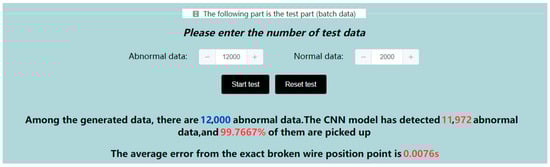
Figure 15.
The final model software test results (12,000 abnormal data points and 2000 normal data points).
At this point, the performance test was still limited to the data generated by the algorithm, and the reliability of the model needed to be further verified using the wire break data measured in the actual test. Using the software to read the real data stored in the software backend through a specific channel for testing, the final model detected all 118 anomalies, with an average error of 0.0695 s.
9. Model Comparison
To confirm the performance of the CNN model built in this study, three models, namely, the BP neural network, SVR (support vector product), and DT (decision tree), were selected for a comparison with this study model. Here, classification was not considered. Only the regression performance was tested using 10,000 algorithm-generated data sets, including 7000 for training and 3000 for testing. The BP neural network uses the same optimizer and activation functions (relu and Adam), with 100 neurons. The SVR model uses linear as the kernel function and the scale function as the sum function coefficients. The DT decision tree has a depth of 10, the number of leaf nodes is 50, and friedman_mse is used as the node splitting evaluation criterion []. The average error of 3000 test data points was calculated (here, the calculation method is the same as that outlined above but with N = 3000), and the settlement results are shown in Figure 16. It can be seen that the average error is as follows: BP > SVR > DT > CNN. The CNN has the highest performance, with an average error of only 0.0452 s. To some extent, this experiment demonstrates the performance of the CNN model in processing one-dimensional data and the effectiveness of the convolutional neural network in regression operations.
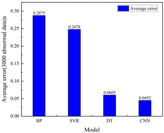
Figure 16.
The average error of the calculation results for the four models.
10. Discussion
From the final test results, we find that the average error of the model, according to the real data, is 0.0874 s greater than that for the algorithm-generated data, which is a reasonable error range. The real data do not perfectly follow the features in the training data set but have a few different fluctuating features due to the experimental conditions [], which affect the computational results of the convolutional neural network.
In this study, we chose to use a combination of a classification model with three regression models, instead of one model, to calculate the results. This choice had two purposes. The first purpose was to reduce the training cost for a single regression model in a case of limited computing power, equivalent to selecting the right medicine for a given ailment, thus reducing the difficulty in training the model and increasing the accuracy of the model. The second purpose was to verify the feasibility of using a convolutional neural network to realize signal classification, because in subsequent research, we will consider other anomalies in addition to broken wires. Thus, the classification of signals is highly necessary. In order to verify the rationality of this choice, we conducted comparative experiments in which we attempted to train a regression model to implement the calculation using a data set of 30,000 data points with a learning rate of 0.001 and other parameters that were identical to those used previously. After obtaining the model, we applied the software module for testing, and the final average error for the data set generated by the algorithm was 0.1312 s for 12,000 data points, which is 0.1236 s greater than that of the model used in this study. In this case, the computing power level and data set level are the same, and the single regression model will still have a high accuracy if the device has very high arithmetic power and is one which further expands the training data set [,,], but it is undeniable that the present model combination performs better than the single model at the same level of arithmetic power. We also tested this single regression model using 118 real broken wire data points, and the final test results are shown in Figure 17b. It can clearly be seen that the error is significantly larger compared to that in Figure 17a. Through the above experiments, we proved that this combination improves the accuracy of the model according to the model logic of classification before calculation with the same level of arithmetic power and that the classification method used for the broken wire data in this study is reasonable and can aid in the regression model calculation.
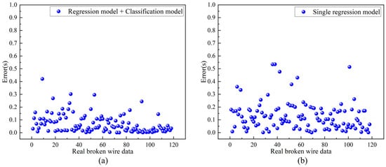
Figure 17.
Test of 118 real broken wire data points. (a) One classification model and three regression models. (b) Single regression model.
On the other hand, the number of data sets required for the performance improvement of convolutional neural networks is relatively large. Of course, this is also related to the epoch; however, blindly increasing the epoch not only requires higher arithmetic power but also renders the process prone to overfitting. Thus, by writing software algorithms to generate broken wire data in bulk, one can yield a greater performance improvement of the neural network, and based on to the current computer hardware performance, the algorithm generating the data is extremely fast, thus saving a great deal of research time. Other studies using convolutional neural networks to identify cable anomalies could also benefit from the model proposed in this paper, which uses the software system to improve the accuracy by more than 10% and simplifies the tedious model testing work in the later stage through the software testing module.
For both the MAE and MSE error functions explored in this study, a general selection method is used. In general, MSE is better than MAE in terms of the computing complexity in solving the gradient, and the gradient is also dynamic and can reach convergence faster and more accurately. However, from the perspective of outliers, if these outliers are actual data or important data, and these outliers must be detected, we should use MSE. On the other hand, is the outliers simply represent corrupted or incorrectly sampled data and need not be given much attention, we should choose MAE as the loss [,]. In this study, if we follow this theory, we should choose MSE, and this is proved by features 2 and 3. However, for feature 1, MAE has a higher performance, and this issue needs to be further explored.
If the model is directly used in the monitoring of actual projects, there will be a problem regarding the data base values, because for different projects and different ties, the design force values are different, and the base values of the signals are different. If this model is applied directly, there will be large deviations. The first method serves to retrain the model based on the new base values, which can be used if the computing power permits it. If there is no training condition, the collected data set can be processed using the unified base value, and the data base value can be changed to the range of the model calculation while retaining its characteristics. In future work, automatic data processing algorithms will be written so as to allow the data to automatically unify the base values as they are fed into the neural network, thus improving the generalizability of the neural network model.
In this study, we proposed a CNN-based method for identifying broken wire signals using an original data generation algorithm to solve the limitation of the data set observed in previous studies, and a complete model testing system was written to accelerate the process of debugging the model parameters during the experiments.
Since broken wires are not the only abnormality in bridge ties, in the next step of this research, we will introduce other abnormal signals and realize the classification of various types of abnormal signals. The implementation method could be improved based on the research described in this paper.
11. Conclusions
In this study, a model combination consisting of one classification model and three regression models was built based on convolutional neural networks, a software system containing two modules for data set generation and model performance testing was developed, and a filament-breaking data generation algorithm was designed in the data set generation phase. The effects of two error functions applied to the model were investigated in the model training phase.
- (1)
- The model successfully detected 11,972 broken wires among 12,000 abnormal data points generated by the algorithm, with a recognition success rate of 99.77% and an average error of 0.0076 s with respect to the location of the broken wire. In the test based on 118 real broken wire data points, the model detected all the abnormalities with an average error of 0.0695 s with respect to the location of the broken wire. In the interference experiment, the model accuracy was 98.56%, the model achieved high-precision broken wire signal recognition.
- (2)
- The generated data algorithm proposed in this study can generate 30,000 random anomalous data points with a length of 200 in approximately just 8.5 s. The performance of the algorithm meets the requirements, and the training results are good and can thus provide a reference for the generation of similar data sets.
- (3)
- In this study, the broken wire data were classified into three categories, and the method of classification before calculation was used. The comparison test showed that the average error of model calculation after classification was 0.1236 s lower than that of direct calculation. The present classification method is reasonable and successfully improves the calculation accuracy of the model at the same level of arithmetic power. In the case of an epoch fixed to 100, for feature 1, it is more suitable to use MAE as the error function, while features 2 and 3 have a higher performance when using the MSE error function. Finally, all three models’ error functions converge to below 0.022.
Author Contributions
This work was carried out in collaboration by all the authors. Conceptualization, W.Z. and R.L.; methodology, R.L. and P.J.; software, R.L.; validation, W.Z., R.L. and P.J.; formal analysis, P.J., J.H. and R.L.; investigation, W.Z.; resources, W.Z.; data curation, P.J.; writing—original draft preparation, W.Z., R.L. and P.J.; writing—review and editing, W.Z. and R.L.; visualization, W.Z. and J.H.; supervision, W.Z.; project administration, W.Z.; funding acquisition, W.Z. All authors have read and agreed to the published version of the manuscript.
Funding
Guangxi Science and Technology Base and Talent Project (No. GUIKE AD20159085) and Natural Science Foundation of China (No. 52068014).
Conflicts of Interest
The authors declare no conflict of interest.
References
- Minaei, A.; Daneshjoo, F.; Goicolea, J.M. Experimental and numerical study on cable breakage equivalent force in cable-stayed structures consisting of low-relaxation seven-wire steel strands. Structures 2020, 27, 595–606. [Google Scholar] [CrossRef]
- Hoang, V.; Kiyomiya, O.; An, T. Experimental and Numerical Study of Lateral Cable Rupture in Cable-Stayed Bridges: Case Study. J. Bridge Eng. 2018, 23, 05018004. [Google Scholar] [CrossRef]
- Lu, N.; Liu, Y.; Beer, M. System reliability evaluation of in-service cable-stayed bridges subjected to cable degradation. Struct. Infrastruct. Eng. 2018, 14, 1486–1498. [Google Scholar] [CrossRef]
- Hao, P.; Yu, C.; Feng, T.; Zhang, Z.; Qin, M.; Zhao, X.; He, H.; Yao, X.S. PM fiber based sensing tapes with automated 45 degrees birefringence axis alignment for distributed force/pressure sensing. Opt. Express 2020, 28, 18829–18842. [Google Scholar] [CrossRef]
- Kim, J.W.; Kim, J.; Park, S. Cross-Sectional Loss Quantification for Main Cable NDE Based on the B-H Loop Measurement Using a Total Flux Sensor. J. Sens. 2019, 2019, 1–10. [Google Scholar] [CrossRef]
- Kim, J.W.; Tola, K.D.; Tran, D.Q.; Park, S. MFL-Based Local Damage Diagnosis and SVM-Based Damage Type Classification for Wire Rope NDE. Materials 2019, 12, 2894. [Google Scholar] [CrossRef] [PubMed]
- Zhang, H.; Li, H.; Zhou, J.; Tong, K.; Xia, R. A multi-dimensional evaluation of wire breakage in bridge cable based on self-magnetic flux leakage signals. J. Magn. Magn. Mater. 2023, 566, 170321. [Google Scholar] [CrossRef]
- Du, W.; Lei, D.; Bai, P.; Zhu, F.; Huang, Z. Dynamic measurement of stay-cable force using digital image techniques. Measurement 2020, 151, 107211. [Google Scholar] [CrossRef]
- Xin, G. Study on the Signal Recognition Method of Brideg Cable Break Based on Acoustic Emission Technology; Shandong University: Jinan, China, 2020. (In Chinese) [Google Scholar]
- Yu, W.; Luo, X.; Qin, H. Experimental Study on Monitoring Cable Broken Wire Signal by FBG Sensor. Laser Optoelectron. Prog. 2023, 60, 0106003. (In Chinese) [Google Scholar] [CrossRef]
- Shinde, P.P.; Shah, S. A Review of Machine Learning and Deep Learning Applications. In Proceedings of the ICCUBEA 2018, Pune, India, 16–18 August 2018. [Google Scholar]
- Jiang, J. BP neural network algorithm optimized by genetic algorithm and its simulation. Int. J. Comput. Sci. Issues IJCSI 2013, 10, 516. [Google Scholar]
- Wu, Y.-C.; Feng, J.-W. Development and Application of Artificial Neural Network. Wirel. Pers. Commun. 2017, 102, 1645–1656. [Google Scholar] [CrossRef]
- Yan, W.; Deng, L.; Zhang, F.; Li, T.; Li, S. Probabilistic machine learning approach to bridge fatigue failure analysis due to vehicular overloading. Eng. Struct. 2019, 193, 91–99. [Google Scholar] [CrossRef]
- Zhang, M.; Zhang, Y.; Gao, Z.; He, X. An Improved DDPG and Its Application Based on the Double-Layer BP Neural Network. IEEE Access 2020, 8, 177734–177744. [Google Scholar] [CrossRef]
- Zhao, Y. Research and Application on BP Neural Network Algorithm. In Proceedings of the 2015 International Industrial Informatics and Computer Engineering Conference (IIICEC 2015), Xi’an, China, 10–11 January 2015. [Google Scholar]
- Feng, J.; Gao, K.; Gao, W.; Liao, Y.; Wu, G. Machine learning-based bridge cable damage detection under stochastic effects of corrosion and fire. Eng. Struct. 2022, 264, 114421. [Google Scholar] [CrossRef]
- Li, Z.; Liu, F.; Yang, W.; Peng, S.; Zhou, J. A Survey of Convolutional Neural Networks: Analysis, Applications, and Prospects. IEEE Trans. Neural Netw. Learn. Syst. 2021, 33, 6999–7019. [Google Scholar] [CrossRef] [PubMed]
- Gu, J.; Wang, Z.; Kuen, J.; Ma, L.; Gang, W. Recent Advances in Convolutional Neural Networks. Pattern Recognit. 2015, 77, 354–377. [Google Scholar] [CrossRef]
- Al, G. Development of a Cable Damage Detection Deep Learning Method based on Acceleration Response of Cable-Stayed Bridge. Turk. J. Comput. Math. Educ. TURCOMAT 2021, 12, 638–647. [Google Scholar] [CrossRef]
- Zhang, Y.; Han, J.; Jing, L.; Wang, C.; Zhao, L. Intelligent Fault Diagnosis of Broken Wires for Steel Wire Ropes Based on Generative Adversarial Nets. Appl. Sci. 2022, 12, 11552. [Google Scholar] [CrossRef]
- Yanwei, W.; Xiaojun, L.; Zifa, W.; Jianping, S.; Enhe, B. Deep learning for P-wave arrival picking in earthquake early warning. Earthq. Eng. Eng. Vib. 2021, 20, 391–402. [Google Scholar] [CrossRef]
- Selim, A.; Paisana, F.; Arokkiam, J.A.; Yi, Z.; Dasilva, L.A. Spectrum Monitoring for Radar Bands using Deep Convolutional Neural Networks. In Proceedings of the GLOBECOM 2017–2017 IEEE Global Communications Conference 2017, Singapore, 4–8 December 2017. [Google Scholar]
- Zhang, Z. Improved Adam Optimizer for Deep Neural Networks. In Proceedings of the 2018 IEEE/ACM 26th International Symposium on Quality of Service (IWQoS), Banff, AB, Canada, 4–6 June 2018. [Google Scholar]
- Li, D.; Mei, H.; Shen, Y.; Su, S.; Zhang, W.; Wang, J.; Zu, M.; Chen, W. ECharts: A declarative framework for rapid construction of web-based visualization. Vis. Inform. 2018, 2, 136–146. [Google Scholar] [CrossRef]
- Charbuty, B.; Abdulazeez, A. Classification Based on Decision Tree Algorithm for Machine Learning. J. Appl. Sci. Technol. Trends 2021, 2, 20–28. [Google Scholar] [CrossRef]
- Xu, J.; Sun, H.; Cai, S. Effect of symmetrical broken wires damage on mechanical characteristics of stay cable. J. Sound Vib. 2019, 461, 114920. [Google Scholar] [CrossRef]
- Xue, Y.; Ray, N.; Hugh, J.; Bigras, G. Cell counting by regression using convolutional neural network. In Proceedings of the Computer Vision–ECCV 2016 Workshops, Amsterdam, The Netherlands, 8–10, 15–16 October 2016; Proceedings, Part I 14, 2016. pp. 274–290. [Google Scholar]
- Miao, S.; Wang, Z.J.; Zheng, Y.; Liao, R. Real-time 2D/3D Registration via CNN Regression. In Proceedings of the 2016 IEEE 13th International Symposium on Biomedical Imaging (ISBI), Prague, Czech Republic, 13–16 April 2016. [Google Scholar]
- Ameri, A.; Akhaee, M.A.; Scheme, E.; Englehart, K. Regression convolutional neural network for improved simultaneous EMG control. J. Neural Eng. 2019, 16, 036015. [Google Scholar] [CrossRef] [PubMed]
- Chicco, D.; Warrens, M.J.; Jurman, G. The coefficient of determination R-squared is more informative than SMAPE, MAE, MAPE, MSE and RMSE in regression analysis evaluation. PeerJ Comput. Sci. 2021, 7, e623. [Google Scholar] [CrossRef]
- Hodson, T.O. Root-mean-square error (RMSE) or mean absolute error (MAE): When to use them or not. Geosci. Model Dev. 2022, 15, 5481–5487. [Google Scholar] [CrossRef]
Disclaimer/Publisher’s Note: The statements, opinions and data contained in all publications are solely those of the individual author(s) and contributor(s) and not of MDPI and/or the editor(s). MDPI and/or the editor(s) disclaim responsibility for any injury to people or property resulting from any ideas, methods, instructions or products referred to in the content. |
© 2023 by the authors. Licensee MDPI, Basel, Switzerland. This article is an open access article distributed under the terms and conditions of the Creative Commons Attribution (CC BY) license (https://creativecommons.org/licenses/by/4.0/).