Blockchain-Based Trusted Federated Learning with Pre-Trained Models for COVID-19 Detection

Abstract

COVID-19 is a serious epidemic that not only endangers human health, but also wreaks havoc on the development of society. Recently, there has been research on using artificial intelligence (AI) techniques for COVID-19 detection. As AI has entered the era of big models, deep learning methods based on pre-trained models (PTMs) have become a focus of industrial applications. Federated learning (FL) enables the union of geographically isolated data, which can address the demands of big data for PTMs. However, the incompleteness of the healthcare system and the untrusted distribution of medical data make FL participants unreliable, and medical data also has strong privacy protection requirements. Our research aims to improve training efficiency and global model accuracy using PTMs for training in FL, reducing computation and communication. Meanwhile, we provide a secure aggregation rule using differential privacy and fully homomorphic encryption to achieve a privacy-preserving Byzantine robust federal learning scheme. In addition, we use blockchain to record the training process and we integrate a Byzantine fault tolerance consensus to further improve robustness. Finally, we conduct experiments on a publicly available dataset, and the experimental results show that our scheme is effective with privacy-preserving and robustness. The final trained models achieve better performance on the positive prediction and severe prediction tasks, with an accuracy of 85.00% and 85.06%, respectively. Thus, this indicates that our study is able to provide reliable results for COVID-19 detection.

1. Introduction

The coronavirus disease 2019 (COVID-19) has brought an unbearable burden and impact on economic development and human life [1]. Extensive clinical experience has shown that chest computed tomography (CT) plays a critical role in the medical diagnosis of COVID-19 patients [2,3]. Some researchers have applied medical image analysis techniques to examine CT images of COVID-19 patients to determine the extent and type of lung lesions [4,5,6,7]. Deep learning technology commonly requires a large amount of sample data to train the model to improve the precision and accuracy of detection. However, sample data from a single source (hospital or research center) is limited and the data distribution is unbalanced, which leads to large errors and a poor generalization ability of the model. Therefore, it is not reliable to train the model considering only local data.

Regulations such as the General Data Protection Regulation (GDPR) place strict restrictions on the collection, storage, and processing of medical data [8]. However, traditional distributed machine learning relies on cloud servers to share local data for model training, but an attacker may invade the server to obtain data without authorization, which inevitably leads to the disclosure of user privacy [9,10,11]. Moreover, vast medical data bring huge computing and storage costs. Therefore, data security, privacy issues, and high costs become obstacles for medical institutions to share data for co-training models.

Google first proposed federated learning in 2016 to achieve the goal of secure data sharing and model joint construction without compromising data privacy [12]. Federated learning combines multiple participants to train a model with their local data, and participants upload model updates to the server for aggregation to generate a global model. In the process of federated learning, local data are not uploaded to the server, which ensures data privacy to a certain extent and reduces transmission and storage costs. The proposal of federated learning can solve the secure sharing of medical data, overcome data islands, and avoid privacy leakages [13,14].

Federated learning is still essentially distributed machine learning, which requires participants to constantly exchange a large number of model parameters with a central server, thus resulting in large communication overhead. Meanwhile, the local model updates submitted by participants may cause user privacy leakages, and unreliable participants may upload incorrect model parameters to destroy the aggregation process and poison the global model. In addition, it also faces the threat of dishonest behavior and having a single point of failure from the central server. Therefore, in order to achieve an efficient, accurate, secure, and trustworthy federated learning solution to better perform the task of CT image detection for COVID-19 patients, we need to address the following problems:

• We generally build complex deep learning models to improve the accuracy of detection, which meets the requirements of training with huge medical data. Therefore, how to reduce the computational and communication overhead of the big model is a problem.
• The medical data has strong privacy attributes, and individuals and society broadly raise the requirements for data security. Therefore, how to strengthen the privacy preserving of medical data and prevent the disclosure of sensitive patient data is an urgent problem.
• The parties participating in federated learning may be untrustworthy, they may accidentally use unprocessed dirty data, or they may intentionally use poisoned data. Therefore, how to identify untrusted participants and avoid global model poisoning is an open problem.
• It is best to record the behavior of untrusted participants and dishonest servers for traceability at anytime. Therefore, how to preserve the training process of federated learning and promote the transparency of cooperative governance is a problem that needs to be solved.

In order to solve the above problems, we propose an effective solution. We introduce pre-training models in federated learning for training, which improves efficiency and accuracy, and reduces the amount of computation and communication. Meanwhile, we use cryptographic methods to protect local data and strengthen privacy and security. In addition, we implement secure aggregation rules with homomorphic encryption algorithms to achieve Byzantine robust federated learning. Finally, we adopt blockchain to document the federated learning training process and Byzantine fault-tolerant consensus to further enhance robustness. Specifically, the key contributions of our work include the following:

• Instead of training new models from scratch, we propose to use pre-trained models in federated learning. The pre-trained models can improve the accuracy of the model and need to train fewer model parameters, which can significantly reduce the training time. Meanwhile, participants only need to upload the parameters of the trained part, which can considerably reduce the communication and computational overhead of the server.
• We propose to use differential privacy mechanisms and homomorphic encryption algorithms to enhance privacy protection. The differential privacy mechanism adds perturbation to the model parameters to prevent untrusted clients or servers from inferring sensitive information of the model updates. The homomorphic encryption algorithm ensures that the calculation process on the server is invisible to the server, which can effectively prevent the malicious behavior of the server.
• Untrusted participants may submit harmful model updates to interfere with the aggregation process and poison the global model. We propose a secure Multi-Krum aggregation algorithm using the CKKS homomorphic encryption scheme. The CKKS algorithm supports fast homomorphism calculation with float numbers, and the Multi-Krum algorithm is based on the Krum aggregation rule, which can filter out abnormal model updates to prevent the global model being poisoned.
• We propose using blockchain to record the federated learning training process. Hyperledger Fabric is a permissioned blockchain that supports smart contract and pluggable consensus protocol, and we use it as a distributed storage to hold the model parameters of each training round. In addition, we integrate the SmartBFL consensus algorithm for it, which further enhances the robustness and has a relatively high efficiency.

The remainder of this paper is organized as follows. In Section 2, we describe previous related works in this area. Then, the system definition, systen design and system analysis of our scheme are introduced in Section 3, Section 4 and Section 5, respectively. Finally, we present the experimental analysis in Section 6 and conclude our work in Section 7.

2. Related Works

With the development of artificial intelligence, many medical image analysis methods based on deep learning models have been proposed, such as U-Net [15], SegNet [16], ViT [17], etc. Both medical image classification and segmentation models can be used for COVID-19 detection [18,19,20,21]. Recently, researchers have proposed applying pre-trained models to detect COVID-19. Gozes et al. [22] proposed using a Resnet-50 neural network pre-trained on the ImageNet database and fine-tuned on the COVID-19 dataset, which finally achieved a high detection accuracy. Gupta et al. [23] proposed adapting the pre-trained models with normalization and regularization techniques, which improved the classification accuracy of the COVID-19 images. Xiao et al. [24] proposed using pre-trained models to predict each slice in patient CT scans and adapt voting mechanisms to compute the final patient prediction result.

The proposal of federated learning solves the problem of data security sharing, and it has also been widely used in the medical field. Kumar et al. [25] proposed a federated learning framework to collect data from different sources and train the global deep learning model. Yang et al. [26] proposed a novel federated semi-supervised learning technique to study the performance gap of model cross prediction on a multi-country database of COVID-19. Dayan et al. [27] proposed a federated learning model that is trained using data from 20 institutions around the world and achieves better sensitivity than training at a single institution. Kandati et al. [28] proposed a novel hybrid algorithm called Genetic CFL, which groups edge devices based on overshoot parameters and modifies the parameter clustering in a genetic manner. Yang et al. [29] proposed federated learning for medical datasets algorithm using partial networks, where only part of the model is shared between the server and client.

Untrusted participants of federated learning may launch poisoning attacks to poison the global model. The classical FedAvg [30] and FedSGD [30] are synthetic schemes vulnerable to poisoning attacks, resulting in unavailability of the global model. Blanchard et al. [31] proposed Krum, a distributed stochastic gradient descent algorithm satisfying the Byzantine resilience. Yin et al. [32] proposed a robust distributed gradient descent algorithm based on median and trimmed mean operations, which has a better robustness and communication efficiency. However, using plaintext to exchange model parameters is vulnerable to inference attacks and causes privacy leakages. Truex et al. [33] proposed a federated learning method that combines differential privacy with secure multi-party computation to prevent inference attacks and maintain a high accuracy of the model. Wibawa et al. [34] proposed a privacy-preserving federated learning algorithm for medical data based on homomorphic encryption, which uses a secure multi-party computation protocol to protect deep learning models from adversaries. Miao et al. [35] proposed a privacy-preserving Byzantine robust federated learning scheme, which utilizes fully homomorphic encryption to compute cosine similarity to provide secure aggregation.

Blockchain is a decentralized ledger technology that can be combined with federated learning to build trusted AI systems. Qu et al. [36] proposed a novel blockchain-enabled federated learning scheme that enables autonomous machine learning using the Proof-of-Work consensus mechanism. Shayan et al. [37] proposed a fully decentralized peer-to-peer multi-party machine learning approach that uses blockchain and cryptographic primitives to coordinate the privacy-preserving machine learning process among peer customers. Nguyen et al. [38] presented a novel blockchain-based federated learning framework for secure COVID-19 data analytics that achieves la ow runtime latency through a decentralized federated learning process and a novel mining solution. Yang et al. [39] proposed a decentralized blockchain-based federated learning architecture to defend against malicious devices using a secure global aggregation algorithm, and deploying a practical Byzantine fault-tolerant consensus protocol among multiple edge servers to prevent model tampering from malicious servers. Islam et al. [40] proposed a federated learning scheme combining drones and blockchain, which achieves a secure accumulation through a two-stage authentication mechanism, and introduces a differential privacy protection mechanism to improve the privacy of the model.

In

Table 1. Comparison between our work and previous works.

Study	A	B	C	D	E	F
Gozes et al. [22]		✓
Kumar et al. [25]	✓				✓
Blanchard et al. [31]				✓
Wibawa et al. [34]	✓		✓
Miao et al. [35]			✓	✓
Shayan et al. [37]			✓	✓
Nguyen et al. [38]	✓		✓
Yang et al. [39]				✓	✓	✓
Ours	✓	✓	✓	✓	✓	✓

A: Federated Learning for COVID-19. B: Training with Pre-Trained Models. C: Privacy-Preserving Mechanism. D: Byzantine Resilient Aggregation. E: Permissioned Blockchain. F: Byzantine Fault Tolerance Consensus.

, we summarize the comparison of our work with previous works on several key features.

3. System Definition

In this section, we formalize the system architecture, federated learning model, threat model, and design objective, respectively.

3.1. System Model

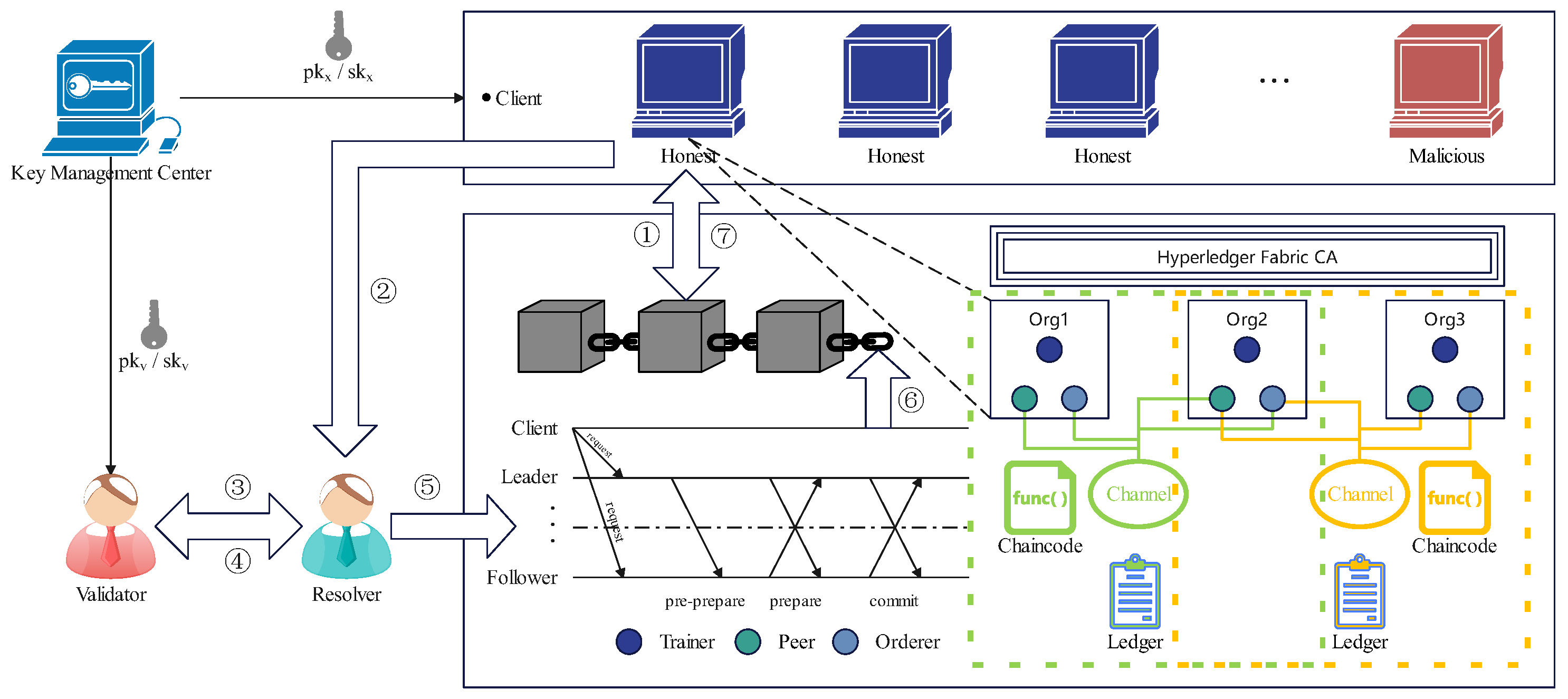
In our study, we consider the goal of multiple medical institutions cooperating to jointly diagnose the condition of COVID-19 patients by designing a trusted federated learning system. As shown in Figure 1, the system capabilities are provided by the federated learning system and Blockchain system:

(1) federated learning system:

• Key Management Center (KMC): A third-party trusted authority responsible for managing and distributing the public/private key pairs of client and validator.
• Client: As the data owner and federated learning participant, the client holds the public and private key pair $({pk}_x,{sk}_x)$ published by the KMC, aiming to benefit from the best global model through collaborative training.
• Trainer: It uses the client’s local data to perform specific federated learning tasks to obtain local model updates.
• Resolver: This is an honest but curious central server which is responsible for collecting the gradient information submitted from the client and executing the gradient validating and filtering.
• Validator: This is another honest but curious and non-collusive central server holding a pair of public/private keys $({pk}_v,{sk}_v)$ published by the KMC, which collaborates with the resolver to compute gradient validating and filtering.

(2) blockchain system:

• Hyperledger Fabric CA: This is the default CA Server component and is used to issue PKI-based certificates to the organization’s members and users.
• Organization: This is authorized to join the blockchain network, also known as the “member”, and performs transactions by the peer nodes.
• Peer: Owned by the organization’s members, this maintains the ledger and uses a chaincode container to perform read and write operations.
• Orderer: This provides an ordering service for all channels on the network and packages transactions into a block for distribution to the connected peer nodes for verification and submission.
• Channel: Each channel in the network corresponds to a ledger, which is shared by all peer nodes in the channel. The transaction parties must be authenticated to the channel to interact with the ledger.
• Ledger: This consists of a “blockchain”, which forms the immutable structure, and a “world state”, which stores the value of the current state of the ledger.
• Chaincode: The chaincode, or smart contract, represents the business logic of the blockchain application. Smart contract programmatically accesses the “blockchain” as well as manipulates the “world state” in the ledger.

The two services process is as follows: ① First, the client downloads the global model from the blockchain and decrypts it, then uses the local dataset for training to obtain the local model update. ② Next, the client encrypts the local model using $p{k}_v$ and sends it to the resolver. Meanwhile, the client submits it encrypted with ${pk}_x$ to the blockchain. ③ Subject to the privacy and security requirements, the resolver and the validator work together to validate and filter the local models submitted by the client to obtain a list of trusted users. ④ Based on the trusted user list, the resolver aggregates the filtered local models to obtain the global model, encrypts it with $p{k}_x$, and finally submits it to the blockchain. ⑤ The orderer nodes use the SmartBFL consensus protocol to sort all legitimate transactions in the channel, packages the transactions into blocks, and distributes them to all peer nodes on the channel. ⑥ Each peer node in the channel independently verifies each transaction in the block to ensure that the ledger remains consistent, executes legitimate transactions. and writes to the ledger upon passing the verification, while the global model is updated. ⑦ Repeat the above procedures (①–⑥) until the global model on the channel reaches convergence.

3.2. FL Model

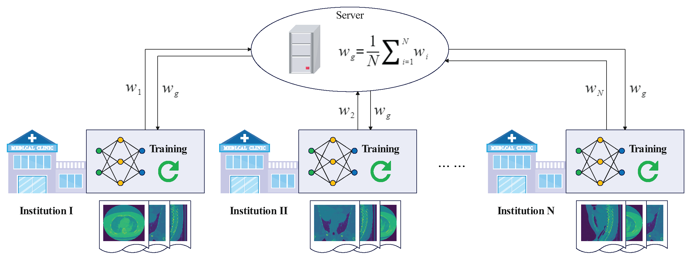
In a standard federated learning (FL) model, there is a central server and N participants $\mathcal{P}=\{p_1,p_2,\cdots ,p_N\}$, each of which owns a local dataset $\mathcal{D}=\{{\mathcal{D}}_1,{\mathcal{D}}_2,\cdots ,{\mathcal{D}}_N\}$. These N participants intend to cooperatively train a global model $\mathit{w}$ without sharing the local datasets, as shown in Figure 2. In the training of round r, participant $p_i$ first downloads the global model ${\mathit{w}}_g^{r-1}$ as local model ${\mathit{w}}_i^{r-1}$ from the server, and then uses the local dataset ${\mathcal{D}}_i$ to train a new local model ${\mathit{w}}_i^r$. The objective function to be optimized for training is:

$$F({\mathit{w}}_i^{r-1},x,y)=\underset{{\mathit{w}}_i^{r-1}}{\min }{\mathbb{E}}_{(x,y)\in {\mathcal{D}}_i}L({\mathit{w}}_i^{r-1},x,y)$$

(1)

where x and y represent the feature and label of the dataset, respectively, L is the loss function, and ${\mathcal{D}}_i$ is the local dataset of party $p_i$. The participant $p_i$ updates the local model using a stochastic gradient descent algorithm as:

$${\mathit{w}}_i^r={\mathit{w}}_i^{r-1}-\eta ·\nabla L({\mathit{w}}_i^{r-1},{\mathcal{D}}_i)$$

(2)

After completing a round of training, participant $p_i$ sends the new local model ${\mathit{w}}_i^r$ to the server. The server collects the local models of the N participants and aggregates them according to Equation (3) to generate a new global model.

$${\mathit{w}}_g^r=\sum _{i=1}^N\frac{|{\mathcal{D}}_i|}{\left|\mathcal{D}\right|}·{\mathit{w}}_i^r$$

(3)

3.3. ViT Model

The local model training of the participants relies on pre-trained models with the vision transformer (ViT) architecture, as illustrated in Figure 3. A 2-D image $\mathit{x}$ is divided into N small patches, each of which is made up of $P\times P$ pixels. Each piece is flattened into a vector that is used as the input sequence, and the linear projection layer receives the input sequence to generate patch embeddings. A learnable class embedding is added to the sequence header. Several embedding techniques utilized by the vision transformer model are available here:

Patch Embedding: To process 2-D images, the image $\mathit{x}\in {\mathbb{R}}^{H\times W\times C}$ is converted into 2-D image patches ${\mathit{x}}_p\in {\mathbb{R}}^{N\times (P^2·C)}$, where $H\times W$ is the resolution of the original image, C is the number of channels, $P^2$ is the resolution of each image patch, and $N=\frac{H\times W}{P^2}$ is the number of patches. Then, the image patches ${\mathit{x}}_p$ are mapped to the D-dimensional vectors ${\mathit{x}}_p\mathit{E}$ via Equation (4), where ${\mathit{x}}_p^n(n\in 1\mathrm{to}N)$ is the image patch and is the image patch and $\mathit{E}$ is a trainable linear projection, and its output is presented as the patch embeddings.

Class Embedding: A learnable class embedding ${\mathit{x}}_{\mathrm{class}}$ is added to the patch embeddings, as shown in Equation (4). The class embedding ${\mathit{x}}_{\mathrm{class}}$ is appended to the 0-th position, i.e., ${\mathit{z}}_0^0$. At the output of the transformer encoder, a classification head is appended to ${\mathit{z}}_L^0$, which is implemented by an MLP, as formulated in Equation (4).

Position Embedding: To preserve the position information, position embedding is added to the patch embeddings, which is used to represent the position by the 1-D position encoding ${\mathit{E}}_{\mathrm{pos}}$ as in Equation (4), and the output ${\mathit{z}}_0$ is sent into the transformer encoder.

$$\left\{\begin{array}{c}{\mathit{z}}_0=[{\mathit{x}}_{\mathrm{class}};{\mathit{x}}_p^1\mathit{E};{\mathit{x}}_p^2\mathit{E};\cdots ;{\mathit{x}}_p^N\mathit{E}]+{\mathit{E}}_{\mathrm{pos}}\hfill \\ \mathit{E}\in {\mathbb{R}}^{(P^2·C)\times D}\hfill \\ {\mathit{E}}_{\mathrm{pos}}\in {\mathbb{R}}^{(N+1)\times D}\hfill \\ \mathit{y}=\mathrm{MLP}\left(\mathrm{LN}\left({\mathit{z}}_L^0\right)\right)\hfill \end{array}\right.$$

(4)

The transformer encoder receives the embeddings as input. It consists of L encoder blocks, where the encoder block is composed of multiple self-attention layer (MSA) and multi-layer perceptron layer (MLP). Then, MSA divides the input into several heads and allows each head to learn different levels of self-attention. Meanwhile, the outputs of all heads are combined and fed to MLP. Besides, layer normalization (LN) is applied before each block and residual connection is applied after each block, as shown in Equation (5):

$$\left\{\begin{array}{c}{\mathit{z}}_{\ell }^{\prime }=\mathrm{MSA}\left(\mathrm{LN}\left({\mathit{z}}_{\ell -1}\right)\right)+{\mathit{z}}_{\ell -1}\hfill \\ {\mathit{z}}_{\ell }=\mathrm{MLP}\left(\mathrm{LN}\left({\mathit{z}}_{\ell }^{\prime }\right)\right)+{\mathit{z}}_{\ell }^{\prime }\hfill \\ \ell =1\cdots L\hfill \end{array}\right.$$

(5)

After extracting the features through the transformer encoder, the classification head ${\mathit{z}}_L^0$ of the last transformer block is used as the feature vector $X_{lung}$, which is concatenated with the age vector $X_{age}$ and the sex vector $X_{sex}$ to form the final feature vector $X_{feature}$. Finally, a logistic regression is applied to output the final prediction ($P_{positive}$ or $P_{severe}$) using the sigmoid function $\sigma \left(x\right)=\frac{1}{1+e^{-x}}$.

3.4. Threat Model

All participants in federated learning want to obtain a global model that performs better than the local models, which motivates them to share the local models trained on their local dataset to co-train the global model. However, participants can be untrustworthy, which means they may launch poisoning attacks to poison the global model. Moreover, participants may launch inference attacks to infer sensitive information from the shared local models. In addition, honest servers may launch model extraction attacks to improperly exploit the model to gain benefits. Finally, participants should be authorized to join the federated learning system after strict certification. Accordingly, the potential threats to our scheme are as follows:

Threat 1: Poisoning attack. Malicious clients can launch poisoning attacks in a variety of ways, with the goal of breaking the correctness of federated learning by tampering with the original data or submitting incorrect local models without being detected.

Threat 2: Inference attack. Although participants in federated learning only use their local data to train local models and only share the local models with other participants, it is still possible for untrusted participants to launch inference attacks to infer sensitive information from the shared local models, leading to privacy leakages.

Threat 3: Model extraction attack. Although the responsible server is assumed to perform the federated learning aggregation process honestly, it may launch model extraction attacks and secretly exploit the model for improper benefits.

Threat 4: Permission control. During the federated learning process, the local models of all participants are shared, and their owner loses control of them, which is likely to be shared by untrusted participants to other unauthorized entities, resulting in data leakage.

3.5. Design Objective

Our proposed goal is to implement a trusted federated learning scheme based on blockchain technology, which can provide privacy protection and data security capabilities, resist poisoning attacks, inference attacks, and model extraction attacks, and can mitigate computational and communication overhead. Meanwhile, our scheme should have approximately the same accuracy as the standard federated averaging algorithm. Specifically, our scheme is designed with the following objectives:

Objective 1: Robustness. The proposed scheme can resist malicious attacks and keep the accuracy of the global model from malicious attack, and all behaviors need to be recorded to prevent malicious participants from being rejected.

Objective 2: Privacy. The proposed scheme can protect the privacy of users from being leaked, and avoid third parties or malicious parties from accessing the original data or inferencing sensitive information from the shared models.

Objective 3: Security. The proposed scheme can protect the user’s data security, prevent the user’s data and models from being stolen, and protect the legitimate rights and interests of the user from being damaged.

Objective 4: Efficiency. The proposed scheme can support privacy protection while reducing the computational and communication overhead.

Objective 5: Accuracy. The proposed scheme can preserve privacy and resist malicious attacks, while the accuracy of the model should be as unaffected as possible.

4. System Design

In this section, we present the details of our scheme and the algorithmic procedures. In

Table 2. Summary of main notations.

Notation	Description
${pk}_x/{sk}_x$	A pair of public/private keys of the client
${pk}_v/{sk}_v$	A pair of public/private keys of the validator
N	Number of clients participating in federated learning
$\mathcal{C}$	A set of all clients participating in federated learning
$c_i$	Federated learning participant, client $c_i\in \mathcal{C}$
$\mathcal{D}$	A set of training datasets on all clients
${\mathcal{D}}_i$	Training dataset ${\mathcal{D}}_i\subseteq \mathcal{D}$ on the client $c_i$
b	Batch size
t	Number of local iterations
r	Number of global iterations
$\eta$	Local training learning rate
${\mathit{g}}_i$	Local gradient of the client $c_i$
${\mathit{w}}_i$	Local model of the client $c_i$
${\mathit{w}}_g$	Global model
${⟦{\mathit{w}}_i⟧}_{{pk}_x}$	Encrypted ${\mathit{w}}_i$ with ${pk}_x$
${⟦{\mathit{w}}_i⟧}_{{pk}_v}$	Encrypted ${\mathit{w}}_i$ with ${pk}_v$
${⟦{\mathit{w}}_g⟧}_{{pk}_x}$	Encrypted ${\mathit{w}}_g$ with ${pk}_x$

, we give the main notations in our scheme.

4.1. System Initialization

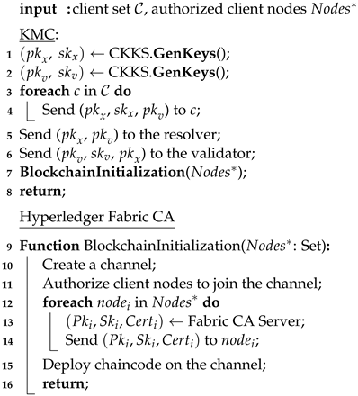
System initialization is divided into the following two parts (See Algorithm 1).

In the initialization phase of the federated learning service, we configure a pair of public/private keys $({pk}_x,{sk}_x)$ for each client node in the system through KMC, and configure another pair of public/private keys $({pk}_v,{sk}_v)$ for the validator. Here, the keys $({pk}_x,{sk}_x)$ and $({pk}_v,{sk}_v)$ are used for the subsequent homomorphic encryption computation. Then, we released two federated learning tasks, one for predicting the probability of the COVID-19 disease and the other for predicting the probability of COVID-19 disease severity. Meanwhile, we submit the original global model to the blockchain.

When the blockchain service is initialized, we create a channel for each federated learning task through the blockchain network. Next, we add orderer nodes, peer nodes, and organization members to the channel, and deploy the chaincode program. At the same time, the Hyperledger Fabric CA issues keys and certificates $({Pk}_i,S{k}_i,{Cert}_i)$ for each node authorized to join the channel. Finally, we generate a genesis block for this channel and store the original global model block on the blockchain. In this way, each federated learning task can be run through these nodes on the corresponding channel of the blockchain.

Algorithm 1: SystemInitialization

4.2. Local Model Training

When a client $c_i$ participating in a federated learning task starts to perform a round of local training, they first downloads the last round of global model ${⟦{\mathit{w}}_g^{r-1}⟧}_{p{k}_x}$ from the blockchain through peer nodes and decrypt it using ${sk}_x$, which then serves as the local model ${\mathit{w}}_i^{r-1}$ for the new round of the training process. Then, the client $c_i$ sends the local model ${\mathit{w}}_i^r$ and the local dataset ${\mathcal{D}}_i$ to the trainer, which is responsible for performing the local model training task (See Algorithm 2).

The trainer performs the local training process through the mini-batch SGD (Stochastic Gradient Descent) algorithm. We define $\mathcal{L}$ as the loss function on a batch size b of samples $X\subset {\mathcal{D}}_i$, then:

$$\mathcal{L}({\mathit{w}}^{t-1},X)=\frac{1}{b}{\sum }_{x\in X}\ell \left({\mathit{w}}^{t-1},x\right)$$

(6)

where x represent the feature and label for a certain sample and $\ell \left({\mathit{w}}^{t-1},x\right)$ is the loss function on a single sample. Therefore, we obtain the local gradient

$${\mathit{g}}^t=\nabla \mathcal{L}({\mathit{w}}^{t-1},X)$$

(7)

and update the local model

$${\mathit{w}}^t={\mathit{w}}^{t-1}-\eta ·{\mathit{g}}^t$$

(8)

through the SGD optimization algorithm, where ∇ is the derivative operation and $\eta$ is the local training learning rate.

Algorithm 2: LocalModelTraining

To enhance the privacy of local training, we integrate a $(ϵ,\delta )$-differential privacy scheme for the trainer. Furthermore, we achieve a DP-SGD gradient perturbation algorithm implemented by the Gaussian mechanism, where Gaussian noise is added to the gradient during local training. We need to determine a Gaussian distribution $\mathcal{N}(0,{\sigma }^2)$ to generate Gaussian noise for applying the Gaussian mechanism.

We set appropriate hyperparameters $ϵ,\delta ,z,C$ satisfying

$$\left\{\begin{array}{c}ϵ\ge \frac{\sqrt{2·ln(1.25/\delta )}}{\sigma /{\Delta }_{2}f}\hfill \\ {\Delta }_{2}f\le C\hfill \\ z=\sigma /C\hfill \end{array}\right.$$

(9)

where z is the noise multiplier, C is the gradient clipping parameter, ${\Delta }_{2}f$ is the sensitivity of the gradient, and $(ϵ,\delta )$ represent the $(ϵ,\delta )$-differential privacy. Then, we have

$$\left\{\begin{array}{c}z=\frac{\sqrt{2·ln(1.25/\delta )}}{ϵ}\hfill \\ \sigma =z·C\hfill \end{array}\right.$$

(10)

Thus, we only need to set the values of the parameters $ϵ,\delta ,C$ to obtain a Gaussian distribution $\mathcal{N}(0,{\sigma }^2)$, which corresponds to $(ϵ,\delta )$-differential privacy. In a short, we can add Gaussian noise to the gradient in three steps: ① First, we compute the gradient at each sample and clip it to a fixed range $[-C,C]$. ② Then, we add Gaussian noise $\mathit{\zeta }\sim \mathcal{N}(0,{\sigma }^2)$ to the clipped gradient. ③ Finally, we update the model using the gradient with Gaussian noise as follow:

$${\mathit{w}}^t={\mathit{w}}^{t-1}-\eta ·\left(\nabla \mathcal{L}({\mathit{w}}^{t-1},{\mathcal{D}}_b)+\mathit{\zeta }\right)$$

(11)

where $\zeta$ is the Gaussian noise.

4.3. Upload Local Model

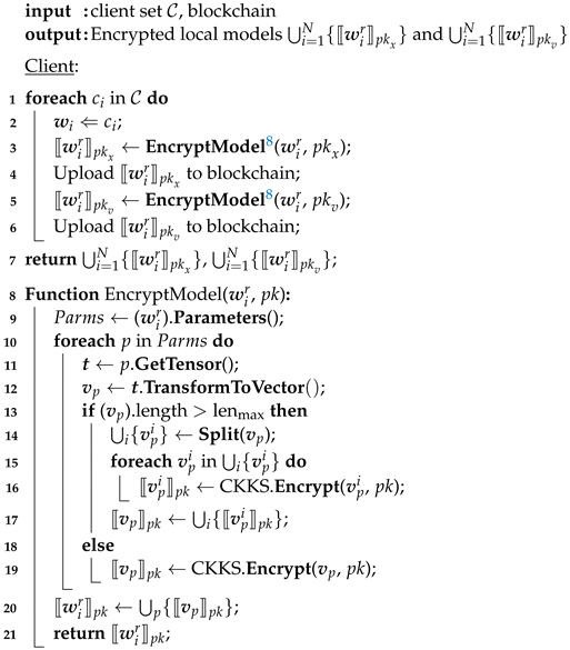
When the trainer completes a round of local training, the client $c_i$ gets the new local model ${\mathit{w}}_i^r$. Before uploading the local model to the resolver and blockchain, we need to encrypt it using homomorphic encryption. Homomorphic encryption is a technique that supports operations over ciphertext without compromising the security of the user data [41]. The classical Paillier [42] semi-homomorphic encryption scheme only supports homomorphic addition and homomorphic scalar multiplication operations in the range of integers, while the second-generation fully homomorphic encryption schemes represented by the BGV scheme [43] and BFV scheme [44] also only support integer operations. Considering that the model parameters are the signed floating-point numbers, it is necessary to quantize and trim the model parameters if these schemes are adopted, which will undoubtedly bring additional computational costs. In contrast, the CKKS [45] fully homomorphic encryption scheme proposed in 2017 supports floating-point addition and multiplication homomorphic operations for real or complex numbers. The calculation results are approximate, which is suitable for machine learning model training and other scenarios that do not require exact results.

Therefore, we choose to encrypt the local model using the CKKS homomorphic encryption scheme. In the details of encryption, we transform the model parameters of the local model into vectors at each layer and encrypt the vectors layer by layer. Furthermore, if the vector is too long to exceed the specified maximum length limit, we split it into multiple vectors and encrypt it multiple times. Specifically, we use the client’s public key ${pk}_x$ and the validator’s public key ${pk}_v$ to encrypt the local model ${\mathit{w}}_i^r$ to gain ${⟦{\mathit{w}}_i^r⟧}_{{pk}_x}$ and ${⟦{\mathit{w}}_i^r⟧}_{{pk}_v}$, respectively. Then, the client $c_i$ uploads ${⟦{\mathit{w}}_i^r⟧}_{{pk}_x}$ and ${⟦{\mathit{w}}_i^r⟧}_{{pk}_v}$ to the blockchain as a transaction, and sends ${⟦{\mathit{w}}_i^r⟧}_{{pk}_v}$ to the resolver at the same time (See Algorithm 3).

Algorithm 3: UploadLocalModel

4.4. Global Model Aggregation

After receiving all clients’ local models, the resolver adopts model averaging approach to aggregate all local models $\left\{{\mathit{w}}_i\right|i=1toN\}$ to obtain the global model ${\mathit{w}}_g$:

$${\mathit{w}}_g=\frac{1}{N}·\sum _{i=1}^N{\mathit{w}}_i$$

(12)

However, some malicious clients may deliberately send wrong local models to interfere with the aggregation process, thereby making the aggregation result invalid and the whole training process fail. In addition, the “honest” but “curious” server (resolver or validator) is likely to infer sensitive information about the client data from the model parameters, which brings concerns about user data privacy. Therefore, we need to consider counteracting the adverse effects of poisoning attacks and protecting the data privacy of the client. In this way, the secure aggregation process may be expressed as:

$${⟦{\mathit{w}}_g⟧}_{{pk}_x}=\frac{1}{N}·\sum _{i=1}^N{⟦{\mathit{w}}_i⟧}_{{pk}_x}$$

(13)

Next, we present some details about the secure aggregation process. We mainly divide global model aggregation into two processes: model filtering and model aggregation (See Algorithm 4).

In the process of model filtering, we adopt a Byzantine robust Multi-Krum aggregation algorithm, which is a popular aggregation rule in distributed machine learning. The Multi-Krum algorithm is a variant of the Krum algorithm and it is resistant to Byzantine attacks. We assume that there is a distributed system consisting of a server and n nodes, in which f nodes may be Byzantine nodes. Each node submits a vector to the server, and the server is responsible for aggregating these vectors. The strategy of the Krum algorithm is to select one of the n vectors that is most similar to the others as the global representative. For any vector v, the Krum algorithm calculates the Euclidean distance between the vector v and other vectors, and selects the nearest $k-f-2$ distances to sum as the score of vector v. Then, the vector with a minimum score is representative of all vectors. The Euclidean distance is calculated as:

$$d=\sqrt{{\sum }_{i=1}^n{(x_i-y_i)}^2}$$

(14)

where d is the Euclidean distance between two n-dimensional vectors ${\mathit{v}}_1=[x_1,x_2,\cdots ,x_n]$ and ${\mathit{v}}_2=[y_1,y_2,\cdots ,y_n]$. The Multi-Krum algorithm uses the same strategy as the Krum algorithm, except that the Multi-Krum algorithm selects m vectors to average as the global representative, which is equivalent to performing m rounds of the Krum algorithm. The two cases $m=1$ and $m=n$ correspond to the Krum algorithm and averaging algorithm.

First, the resolver calculates the Euclidean distance between any two models, ${⟦{\mathit{w}}_i^r⟧}_{p{k}_v}$ and ${⟦{\mathit{w}}_j^r⟧}_{p{k}_v}$. We assume that ${\mathit{w}}_i^r$ and ${\mathit{w}}_j^r$ are two n-dimensional vectors, $\mathit{u}=[u_1,u_2,\cdots ,u_n]$ and $\mathit{v}=[v_1,v_2,\cdots ,v_n]$, respectively. Thus, we can calculate the Euclidean distance between ${\mathit{w}}_i^r$ and ${\mathit{w}}_j^r$ as follows:

$$\begin{array}{c}\hfill dist({\mathit{w}}_i^r,{\mathit{w}}_j^r)=\sqrt{{\sum }_{k=1}^n{(u_k-v_k)}^2}\end{array}$$

(15)

Let $s={\sum }_{k=1}^n{(u_k-v_k)}^2$, then s denotes the sum over all elements of vector $\mathit{w}={[{(u_1-v_1)}^2,{(u_2-v_2)}^2,\cdots ,u_n-v_n)}^2]$. The vector can be calculated from the following:

$$\begin{array}{cc}\hfill \mathit{w}& ={[{(u_1-v_1)}^2,{(u_2-v_2)}^2,\cdots ,u_n-v_n)}^2]\hfill \\ \hfill & =[\mathit{u}-\mathit{v}]\circ [\mathit{u}-\mathit{v}]\hfill \\ \hfill & =[{\mathit{w}}_i^r-{\mathit{w}}_j^r]\circ [{\mathit{w}}_i^r-{\mathit{w}}_j^r]\hfill \end{array}$$

(16)

where the operator ∘ represents the Hadamard product. Hence, we calculate that:

$$\begin{array}{cc}\hfill {⟦\mathit{w}⟧}_{p{k}_v}& ={⟦\left[{\mathit{w}}_i^r-{\mathit{w}}_j^r\right]\circ \left[{\mathit{w}}_i^r-{\mathit{w}}_j^r\right]⟧}_{p{k}_v}\hfill \\ \hfill & ={⟦\left[{\mathit{w}}_i^r-{\mathit{w}}_j^r\right]⟧}_{p{k}_v}\circ {⟦\left[{\mathit{w}}_i^r-{\mathit{w}}_j^r\right]⟧}_{p{k}_v}\hfill \\ \hfill & =\left[{⟦{\mathit{w}}_i^r⟧}_{p{k}_v}-{⟦{\mathit{w}}_j^r⟧}_{p{k}_v}\right]\circ \left[{⟦{\mathit{w}}_i^r⟧}_{p{k}_v}-{⟦{\mathit{w}}_j^r⟧}_{p{k}_v}\right]\hfill \end{array}$$

(17)

Since the CKKS homomorphic encryption scheme not only provides homomorphic addition, subtraction, and multiplication, but also supports ciphertext vector rotation, vector rotation enables the operation of the summing of all the elements of a vector. Let ${\mathit{v}}^{\left(t\right)}$ represent rotating the vector $\mathit{v}=[v_1,v_2,\cdots ,v_n]$ with t times, and then we can obtain:

$$\begin{array}{cc}\hfill {\mathit{v}}^{\left(0\right)}& =[v_1,v_2,\cdots ,v_{n-1},v_n]\hfill \\ \hfill {\mathit{v}}^{\left(1\right)}& =[v_2,v_3,\cdots ,v_n,v_1]\hfill \\ \hfill & \cdots \hfill \\ \hfill {\mathit{v}}^{\left(t\right)}& =[v_{t+1},v_{t+2},\cdots ,v_{t-1},v_t]\hfill \\ \hfill & \cdots \hfill \\ \hfill {\mathit{v}}^{(n-1)}& =[v_n,v_1,\cdots ,v_{n-2},v_{n-1}]\hfill \\ \hfill {\mathit{v}}^{\left(n\right)}& =[v_1,v_2,\cdots ,v_{n-1},v_n]\hfill \end{array}$$

(18)

Algorithm 4: GlobalModelAggregate

Furthermore, when rotating the vector $\mathit{w}$ for $n-1$ times, we obtain:

$$\begin{array}{cc}\hfill {\mathit{w}}^{\left(0\right)}& =[{(u_1-v_1)}^2,{(u_2-v_2)}^2,\cdots ,{(u_n-v_n)}^2]\hfill \\ \hfill {\mathit{w}}^{\left(1\right)}& ={[{(u_2-v_2)}^2,\cdots ,{(u_n-v_n)}^2,u_1-v_1)}^2]\hfill \\ \hfill & \cdots \hfill \\ \hfill {\mathit{w}}^{(n-2)}& =[{(u_{n-1}-v_{n-1})}^2,\cdots ,{(u_{n-2}-v_{n-2})}^2]\hfill \\ \hfill {\mathit{w}}^{(n-1)}& =[{(u_n-v_n)}^2,\cdots ,{(u_{n-1}-v_{n-1})}^2]\hfill \end{array}$$

(19)

Then, we sum ${\mathit{w}}^{\left(0\right)},{\mathit{w}}^{\left(1\right)},\cdots ,{\mathit{w}}^{(n-1)}$ and obtain:

$$\begin{array}{cc}\hfill {\displaystyle \sum _{t=0}^{n-1}}{\mathit{w}}^{\left(t\right)}& ={\mathit{w}}^{\left(0\right)}+{\mathit{w}}^{\left(1\right)}+\cdots +{\mathit{w}}^{(n-1)}\hfill \\ \hfill & =\left[\stackrel{n\mathrm{items}}{\overbrace{{\displaystyle \sum _{k=1}^n}{(u_k-v_k)}^2,\cdots ,{\displaystyle \sum _{k=1}^n}{(u_k-v_k)}^2}}\right]\hfill \\ \hfill & =\left[\stackrel{n\mathrm{items}}{\overbrace{s,s,\cdots ,s,s}}\right]\hfill \\ \hfill & =\mathit{s}\hfill \end{array}$$

(20)

Following the above process, we can obtain:

$$\begin{array}{cc}\hfill {⟦\mathit{s}⟧}_{p{k}_v}& ={⟦{\displaystyle \sum _{t=0}^{n-1}}{\mathit{w}}^{\left(t\right)}⟧}_{p{k}_v}\hfill \\ \hfill & ={⟦{\mathit{w}}^{\left(0\right)}+{\mathit{w}}^{\left(1\right)}+\cdots +{\mathit{w}}^{(n-1)}⟧}_{p{k}_v}\hfill \\ \hfill & ={⟦{\mathit{w}}^{\left(0\right)}⟧}_{p{k}_v}+{⟦{\mathit{w}}^{\left(1\right)}⟧}_{p{k}_v}+\cdots +{⟦{\mathit{w}}^{(n-1)}⟧}_{p{k}_v}\hfill \\ \hfill & ={⟦\mathit{w}⟧}_{p{k}_v}^{\left(0\right)}+{⟦\mathit{w}⟧}_{p{k}_v}^{\left(1\right)}+\cdots +{⟦\mathit{w}⟧}_{p{k}_v}^{(n-1)}\hfill \\ \hfill & ={\displaystyle \sum _{t=0}^{n-1}}{⟦\mathit{w}⟧}_{p{k}_v}^{\left(t\right)}\hfill \\ \hfill & ={\displaystyle \sum _{t=0}^{n-1}}{\left(\left[{⟦{\mathit{w}}_i^r⟧}_{p{k}_v}-{⟦{\mathit{w}}_j^r⟧}_{p{k}_v}\right]\circ \left[{⟦{\mathit{w}}_i^r⟧}_{p{k}_v}-{⟦{\mathit{w}}_j^r⟧}_{p{k}_v}\right]\right)}^{\left(t\right)}\hfill \end{array}$$

(21)

Therefore, we are able to compute ${⟦\mathit{s}⟧}_{p{k}_v}$ by homomorphic addition, multiplication and rotation. Since $dist({\mathit{w}}_i^r,{\mathit{w}}_j^r)=\sqrt{{\sum }_{k=1}^n{(u_k-v_k)}^2}=\sqrt{s}$, we are not able to obtain ${⟦dist({\mathit{w}}_i^r,{\mathit{w}}_j^r)⟧}_{p{k}_v}$ directly. In fact, there is no need to calculate the Euclidean distance between ${\mathit{w}}_i^r$ and ${\mathit{w}}_i^r$, as we can merely use the square of the distance.

After completing the calculation of the Euclidean distance between any two local models, the resolver sends the result to the validator, which is the square of the distance, and the validator decrypts the result with the secure key $s{k}_v$. Then, the validator sorts the set of distances corresponding to each model in ascending order and takes the sum of the first k distances to obtain a score ($k=n-f-2+1$, where “+1” represents the distance between the model and itself).Next, the validator adds the client corresponding to the model with a minimum score to the selected clients set and removes it from the candidate clients set. Finally, the validator repeats the above process m times to add m items to the selected set. When finished, the validator sends the last selected clients to the resolver.

In the process of model aggregation, the resolver chooses the corresponding local model according to the selected clients set to participate in the aggregation process. Specifically, the resolver uses the model averaging algorithm for global model aggregation on all selected models. The model average algorithm is shown as follows:

$$\begin{array}{c}\hfill {\mathit{w}}_g^r=\frac{1}{n}{\displaystyle \sum _{i=1}^n}{\mathit{w}}_i^r\end{array}$$

(22)

Since the model is encrypted, the resolver needs to calculate the global model through homomorphic operations:

$$\begin{array}{cc}\hfill {⟦{\mathit{w}}_g^r⟧}_{p{k}_v}& ={⟦\frac{1}{n}{\displaystyle \sum _{i=1}^n}{\mathit{w}}_i^r⟧}_{p{k}_v}\hfill \\ \hfill & =\frac{1}{n}{⟦{\displaystyle \sum _{i=1}^n}{\mathit{w}}_i^r⟧}_{p{k}_v}\hfill \\ \hfill & =\frac{1}{n}{⟦{\mathit{w}}_1^r+{\mathit{w}}_2^r+\cdots +{\mathit{w}}_n^r⟧}_{p{k}_v}\hfill \\ \hfill & =\frac{1}{n}({⟦{\mathit{w}}_1^r⟧}_{p{k}_v}+{⟦{\mathit{w}}_2^r⟧}_{p{k}_v}+\cdots +{⟦{\mathit{w}}_n^r⟧}_{p{k}_v})\hfill \\ \hfill & =\frac{1}{n}{\displaystyle \sum _{i=1}^n}{⟦\mathit{w}⟧}_{p{k}_v}\hfill \end{array}$$

(23)

In this way, the validator obtains the global model ${⟦{\mathit{w}}_g^r⟧}_{p{k}_v}$. However, the global model is encrypted with the validator’s public key $p{k}_v$ and cannot be used by the client directly. Therefore, the resolver needs to send the global model ${⟦{\mathit{w}}_g^r⟧}_{p{k}_v}$ to the validator for decryption and then is encrypted with the client’s public key $p{k}_x$. In order to avoid privacy leakage issues caused by directly exposing the global model ${\mathit{w}}_g^r$ to the validator, the resolver needs to generate a random vector $\mathit{v}$ for multiplying with the global model ${⟦{\mathit{w}}_g^r⟧}_{p{k}_v}$ and sends product ${⟦\mathit{v}\circ {\mathit{w}}_g^r⟧}_{p{k}_v}$ to the validator. Then, the validator sends ${⟦\mathit{v}\circ {\mathit{w}}_g^r⟧}_{p{k}_x}$ re-encrypted with the client’s public key $p{k}_x$ to the resolver. Finally, the resolver can obtain the global model ${⟦{\mathit{w}}_g^r⟧}_{p{k}_x}$ by calculating $1/\mathit{v}\circ {⟦\mathit{v}\circ {\mathit{w}}_g^r⟧}_{p{k}_x}$.

In the global model aggregation stage, not only the final generated global model needs to be uploaded to the blockchain, but also the resolver and validator need to submit the intermediate results to the blockchain for recording their behavior. This helps to verify the dishonest behavior of the central server and ensure the robustness of the system.

4.5. SmartBFT Consensus

In our decentralized storage design, we adopt Hyperledger Fabric as the underlying blockchain technology. This is an open source distributed ledger technology that is modular, configurable, and supports smart contracts; one of its most attractive features is the design of a pluggable consensus protocol. In v2.0, it provides the Raft consensus protocol, eliminating the Kafka and Solo sorting service. However, in the decentralized scenario, it is necessary to introduce the Byzantine fault tolerance (BFT) consensus protocol, but Hyperledger Fabric lacks support for BFT consensus protocol. Therefore, we decided to adopt the SmartBFT consensus as the solution for the Hyperledger Fabric sorting service.

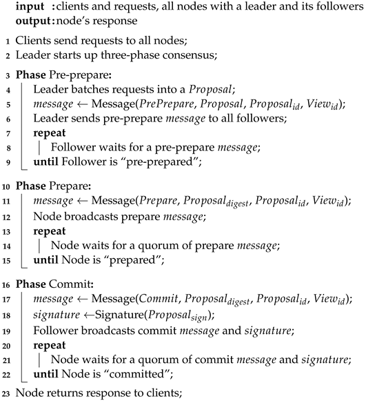
We assume that the number of nodes participating in the consensus is n and that there are at most f Byzantine nodes, so the SmartBFT algorithm can ensure that the system is running safely when at most f nodes fail. The consensus process begins with a client sending requests to all nodes. The leader of the current view batches requests into a proposal and starts executing the three-phase consensus. At the end, at least $n-f$ nodes could submit the proposals, and if a view change is occurring, the proposal will be forwarded to the next view leader. The three-phases of consensus are pre-prepare, prepare and commit as following (See Algorithm 5).

Pre-prepare: In the pre-prepare phase, the leader assembles the requests into a proposal ($Proposal$) in batches, which is then assigned a sequence number ($Proposa{l}_{id}$). Next, the leader sends a pre-prepare message $\langle PrePrepare,$$Proposal,$$Proposa{l}_{id},$$Vie{w}_{id}\rangle$ to all of its followers, which contains the proposal, sequence number, and current view number. If the proposal is valid and the follower has not accepted another different pre-prepare message with the same sequence number and view number, it will accept the pre-prepare message, and once follower accepts a pre-prepare message, it will be “pre-prepared” and enter the prepare phase.

Prepare: The “pre-prepared” follower accepts a pre-prepare message and broadcasts a prepare message $\langle Prepare,$$Proposa{l}_{digest},$$Proposa{l}_{id},$$Vie{w}_{id}\rangle$, which includes the digest of the accepted proposal, sequence number, and current view number. Next, each node waits to receive a quorum of prepare messages with the same digest, sequence number and view number. When the node receives a quorum of prepare messages, it will be “prepared” and enter the commit phase.

Commit: The “prepared” node broadcasts a commit message $\langle Commit,$$Proposa{l}_{digest},$$Proposa{l}_{id},$$Vie{w}_{id}\rangle$ and a signature on the $Proposal$, where the content of the commit message is the same as the prepare message. Then, every node waits to receive a quorum of commit messages and signatures. After receiving a quorum of validated commit messages, the node will be “committed” and deliver its response to the client.

The pre-prepare phase and prepare phase are used to fully order requests sent in the same view, even if there is an error in the leader proposing the order requests. The prepare phase and commit phase are used to ensure that submitted requests are fully order requests across views. After the three-phase consensus, SmartBFL has completed the process of accepting transactions, sorting transactions, and returning transaction blocks by the order nodes.

Algorithm 5: SmartBFTConsensus

4.6. Download Global Model

In the last step, client $c_i$ downloads the latest global model ${⟦{\mathit{w}}_g^r⟧}_{p{k}_x}$ and decrypts it with secure key $s{k}_x$. If the global model ${\mathit{w}}_g^r$ reaches the convergence condition, it indicates that the training is completed and the client $c_i$ will exit the training process and submit the final model, otherwise it will continue with the next round of training (See Algorithm 6).

Algorithm 6: DownloadGlobalModel

5. System Analysis

5.1. Privacy and Security

In the system design, we use Byzantine robustness, differential privacy, homomorphic encryption, and permissioned chain to establish the privacy and security mechanisms for federated learning participants against threat issues.

• The Multi-Krum aggregate rule is able to resist the threat of poisoning attack launching by malicious participants. In order to poison the global model, malicious participants upload malicious models to the server to participate in the aggregation process, and the malicious model behaves far away from the general benign model on the vector space. By calculating the Euclidean distance between each model, we select models that are similar to majority models to aggregate the global model, thereby filtering out malicious models. Therefore, when the proportion of malicious actors is not dominant, the Multi-Krum algorithm is able to guarantee the robustness of the global model without affecting the normal convergence.
• The ($ϵ$, $\delta$)-differential privacy mechanism can prevent the threat caused by an inference attack. The model contains the knowledge of the training data from which we can infer sensitive information of users, leading to privacy leakage. Differential privacy proposes a strict definition of privacy protection, and we satisfy the constraint of differential privacy through the noise mechanism. Meanwhile, differential privacy is transitive; that is, for a random algorithm $\mathcal{M}$ satisfying ($ϵ$, $\delta$)-DP, the new algorithm $f\circ \mathcal{M}$ constituted by any form of processing on its result also satisfies ($ϵ$, $\delta$)-DP. In the training process, we trim the gradient and add Gaussian noise to it, then the gradient with noise also has the characteristic of differential privacy, which can be passed to the subsequent inference process.
• The CKKS fully homomorphic encryption scheme avoids the threat of a model extraction attack while strengthening the protection of data security. It provides a homomorphic operation based on floating-point numbers, which we adopt to encrypt the model. Since the model is encrypted and stored in the blockchain, anyone who does not hold the decryption key will not be able to decrypt the plaintext model from it during transmission and aggregation. Meanwhile, we set two non-colluding servers to execute the Multi-Krum algorithm on the encrypted models to prevent the servers from stealing the plaintext models.
• The permissioned blockchain provides the functions of member management and data management. The users with permission can upload or download models stored in the blockchain, while others cannot access the models. Meanwhile, the models stored in the blockchain can only be added and queried, but not deleted or modified, which is supported by the tamper-proof feature of the blockchain. In addition, anyone with audit authority can access the historical models stored in the blockchain for model verification.

In summary, our scheme is able to provide the protection of privacy and security in federated learning.

5.2. Convergence Analysis

In our scheme, the differential privacy mechanism introduces some noise to the model, and the Multi-Krum aggregation algorithm filters out a part of possible malicious models. These operations can impact the performance of the global model, so we mainly discuss their impact on the convergence of the global model. Note that the CKKS scheme only produces almost forgotten noise and has little impact on the performance of the global model, so it is not discussed here.

First, we discuss the convergence of federated learning under differential privacy. To analyze the convergence of DP-SGD in the non-convex setting, we follow the standard assumptions in the SGD [46]. For convenience, we make the following assumptions:

Assumption 1 

(Lower bound of loss). For $\forall \mathit{w}$ and some constant ${\mathcal{L}}^{*}$, we have $\mathcal{L}\left(\mathit{w}\right)\ge {\mathcal{L}}^{*}$.

Assumption 2 

(Smoothness). Let $\mathit{g}\left(\mathit{w}\right)$ denote the gradient of the objective $\mathcal{L}\left(\mathit{w}\right)$. For $\forall \mathit{w},\mathit{v}$, there is a non-negative constant L such that

$$\mathcal{L}\left(\mathit{v}\right)\le \mathcal{L}\left(\mathit{w}\right)+\mathit{g}{\left(\mathit{w}\right)}^{\top }(\mathit{v}-\mathit{w})+\frac{L}{2}{\parallel \mathit{w}-\mathit{v}\parallel }^2$$

(24)

Assumption 3 

(Gradient noise). The per-sample gradient noise ${\tilde{\mathit{g}}}_{t,i}-{\mathit{g}}_t$ is i.i.d. from some distribution, such that

$$\left\{\begin{array}{c}\mathbb{E}({\tilde{\mathit{g}}}_{t,i}-{\mathit{g}}_t)=0\hfill \\ \mathbb{E}\parallel {\tilde{\mathit{g}}}_{t,i}-{\mathit{g}}_t{\parallel }^2\le {\xi }^2\hfill \end{array}\right.$$

(25)

Theorem 1. 

Under Assumptions 1–3, running DP-SGD with clipping for T iterations and setting the learning rate $\eta \propto 1/\sqrt{T}$ give

$$\begin{array}{cc}\hfill \underset{0\le t\le T}{\min }\mathbb{E}(\parallel {\mathit{g}}_t\parallel )& \le \mathcal{G}\left(\frac{4}{\sqrt{T}}\sqrt{({\mathcal{L}}_0-{\mathcal{L}}_{*})L\left(1+\frac{{\sigma }^{2}d}{B^2}\right)};\xi ,\gamma \right)\hfill \\ \hfill & =\underset{r>0}{\min }\frac{\xi }{r}+\mathcal{F}\left(\Delta ;r,\xi ,\gamma \right).\hfill \end{array}$$

(26)

where Δ represents the first argument of $\mathcal{G}$, and $\mathcal{G}$ is increasing and positive. As $T\to \infty$, we have ${\min }_t\mathbb{E}(\parallel {\mathit{g}}_t\parallel )=O\left(T^{-1/4}\right)$, the same rate as the standard SGD.

For the proof, see Appendix A.1.

Remark 1. 

In Theorem 1, the upper bound takes an implicit form of $\mathcal{G}(\Delta ;\xi ,\gamma )$ because it is a lower envelope of functions $\frac{\xi }{r}+\mathcal{F}(\Delta ;r,\xi ,\gamma )$ over all possible $r>0$, whose forms are detailed in Theorem 1. Notice that $\mathcal{G}$ results only from the clipping operation, not from the noise addition.

Next, we discuss the convergence of federated learning with the Multi-Krum algorithm. Since the Multi-Krum algorithm is an extension of the Krum algorithm, their convergence properties are consistent. Therefore, we only need to analyze the convergence of the Krum algorithm. We first introduce the definitions of Byzantine resilience and Krum.

Definition 1 

($\Delta$-Byzantine resilience). Assume that $0\le q\le m$. Let $\{v_i:i\in \left[m\right]\}$ be any i.i.d. random vectors in ${\mathbb{R}}^d$, $v_i\sim G$, with $\mathbb{E}\left[G\right]=g$. Let $\{{\tilde{v}}_i:i\in \left[m\right]\}$ be the set of vectors, of which up to q of them are replaced by arbitrary vectors in ${\mathbb{R}}^d$, while the others are still equal to the corresponding $\left\{v_i\right\}$. Aggregation rule $\mathrm{Agg}(·)$ is said to be Δ-Byzantine resilient if

$$\mathbb{E}\parallel \mathrm{Agg}\left(\{{\tilde{v}}_i:i\in \left[m\right]\}\right){-g\parallel }^2\le \Delta ,$$

(27)

where Δ is a constant dependent on m and q.

Definition 2 

(Krum). We choose the vector with the minimal local sum of distances:

$$\mathrm{Krum}\left(\{{\tilde{v}}_i:i\in \left[m\right]\}\right)={\tilde{v}}_k,k={\mathrm{argmin}}_{i\in \left[m\right]}\sum _{i\to j}{\parallel {\tilde{v}}_i-{\tilde{v}}_j\parallel }^2,$$

(28)

where $i\to j$ are the indices of the $m-q-2$ nearest neighbors of ${\tilde{v}}_i$ in $\{{\tilde{v}}_i:i\in \left[m\right]\}$ measured by the Euclidean distance.

The Krum algorithm is $\Delta$-Byzantine resilient under certain assumptions. Therefore, we provide the convergence guarantees for SGD with $\Delta$-Byzantine-resilient aggregation rules. We follow the assumption of $L_F$-smooth in convergence analysis and prove the convergence of SGD for general smooth and non-convex loss functions.

Assumption 4 

(Smoothness). If $F\left(x\right)$ is $L_F$-smooth and $L_F\ge 0$, then

$$F\left(y\right)-F\left(x\right)\le {\nabla F\left(x\right)}^T·(y-x)+\frac{L_F}{2}{\parallel y-x\parallel }^2,\forall x,y\in {\mathbb{R}}^d$$

(29)

Theorem 2. 

Underlying Assumption 4, we take $\gamma \le \frac{1}{L_F}$. In any iteration t, the correct gradients are $v_i^t=\nabla F_i\left(x^t\right)$. Using Δ-Byzantine-resilient aggregation rule with corresponding assumptions, we obtain linear convergence with a constant error after T iterations with SGD:

$$\frac{{\sum }_{i=0}^{T-1}\mathbb{E}{\parallel \nabla F\left(x^i\right)\parallel }^2}{T}\le \frac{2}{\gamma T}\left[F\left(x^0\right)-F\left(x^{*}\right)\right]+\Delta .$$

(30)

For the proof, see Appendix A.2.

5.3. Complexity Analysis

We mainly analyze the complexity of our scheme through the computation and communication cost of the servers and the clients. The CKKS fully homomorphic encryption scheme consists of basic operations such as encryption, decryption, addition, multiplication, and rotation. For the plaintext and ciphertext of certain models, we can define the time costs of these basic operations as $T_{enc}$, $T_{dec}$, $T_{add}$, $T_{mul}$, and $T_{rot}$, respectively. At the same time, we set the size of the plaintext model to $S_{pt}$, while $S_{ct}$ is the size of the corresponding ciphertext model. The number of all the clients is n, and the number of the possible Byzantine client is f, so we have $k=n-f-2$. In addition, since the computation and the communication costs generated by the operation and transmission on the plaintext are relatively small, we do not carry out a specific analysis and denote them by the symbols $\tau$ and $\varsigma$, respectively. The computation and communication costs of our proposed scheme are shown in

Table 3. Complexity Analysis of Our Scheme.

Role		Computation Cost	Communication Cost
Clients		$\mathcal{O}\left(T_{enc}+T_{dec}\right)$	$\mathcal{O}\left(S_{ct}\right)$
Servers	Resolver	$\mathcal{O}\left((n^3+n^2+k)·T_{add}+(n^2+3)·T_{mul}+n^3·T_{rot}+\tau \right)$	$\mathcal{O}\left((\frac{n^2-n}{2}+n+3)·S_{ct}+\varsigma \right)$
	Validator	$\mathcal{O}\left(T_{enc}+(\frac{n^2-n}{2}+1)·T_{dec}+\tau \right)$	$\mathcal{O}\left((\frac{n^2-n}{2}+2)·S_{ct}+\varsigma \right)$

. We can conclude that the computation and communication costs of the clients are very limited, so a lot of computing resources can be used to train the models. Servers contract most of the computation and storage overhead, especially resolvers, so we need to allocate sufficient computer resources to them.

6. Experiments and Numerical Results

6.1. Dataset and Experimental Setting

The STOIC project [47] collected and created a large publicly available dataset containing CT images from 10735 patients, which was used to evaluate the value of CT images in the diagnosis and prognosis of COVID-19 pneumonia. The dataset was randomly divided into a public training set (2000 patients), a test set (approximately 1000 patients) and a private training set (more than 7000 patients). Meanwhile, the CT images were stored as files in “*.mha” format.

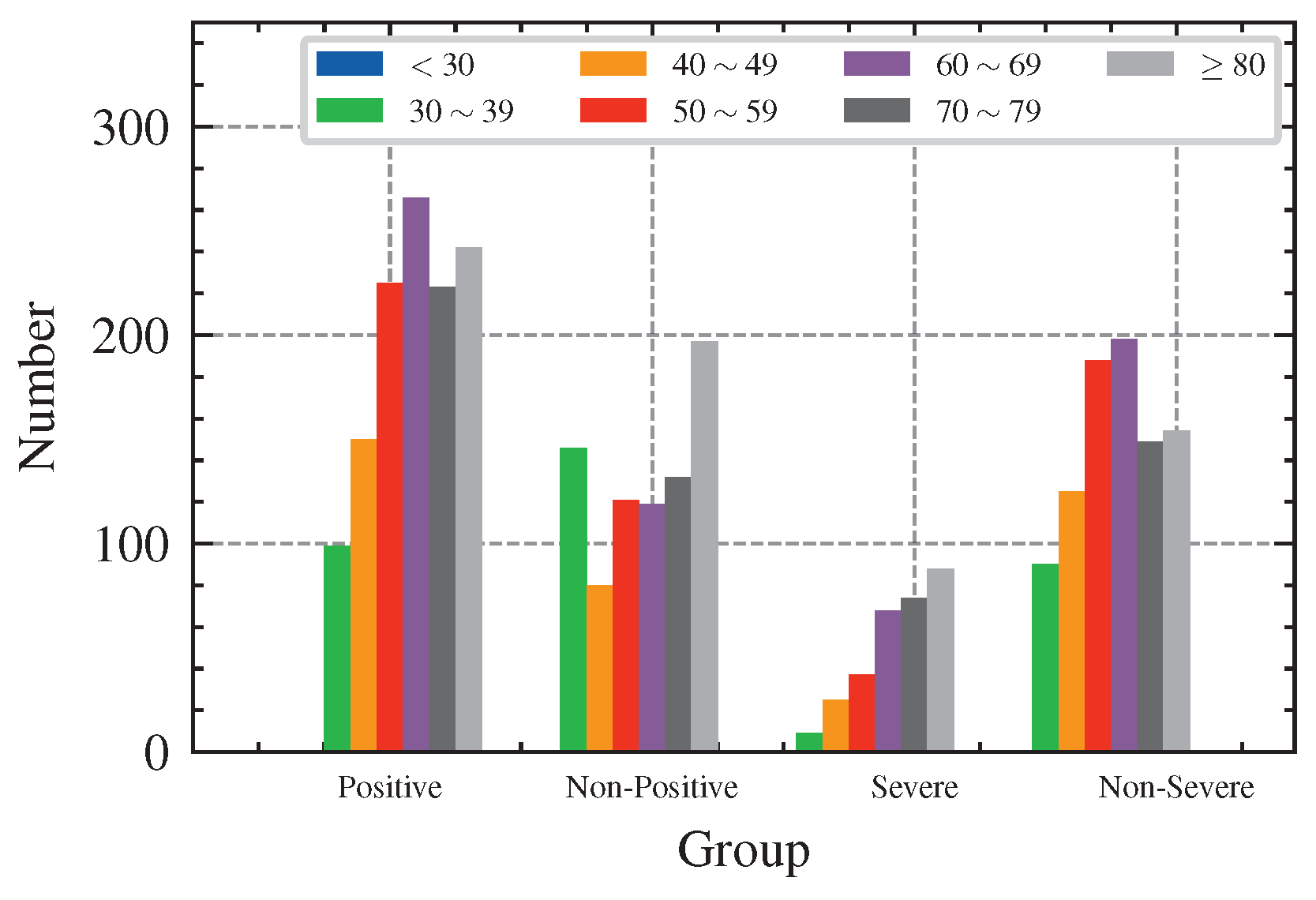
In our work, we conducted research on the STOIC public training set [48], which can be downloaded at https://registry.opendata.aws/stoic2021-training/ (accessed on 30 September 2022). The dataset contains 2000 CT images, where each mha file corresponds to one patient, and the reference.csv file contains labels corresponding to the positive and severity results of COVID-19 indexed by the patient ID. The distribution of the dataset is shown in

Table 4. Distribution of Positive/Non-Positive and Severe/Non-Severe of the Dataset.

Label	Positive	Severity
0	795	904
1	1205	301

, Figure 4 and Figure 5. Note that the data on severity are counted in the case of a confirmed positive, i.e., ${\mathrm{label}}_{\mathrm{positive}}=1$.

Our goal is to input a CT image file of a suspected COVID-19 patient and use the deep learning technique to predict the probability of positive and the probability of the severity of the COVID-19 disease, where severity refers to intubation or death within one month. Thus, we can train two models to predict the probability of positive and the probability of severe, respectively. For this purpose, we first need to pre-process the data to feed into the deep learning model for training. We use the SimpleITK library to transform the mha file by adjusting the scan spacing of the CT image to (1.5 mm, 1.5 mm, 5 mm) and reshaping the shape to $224\times 224\times Z$. Next, we normalize it using the mean and standard deviation of ImageNet and reshape it to $Z\times 3\times 224\times 224$. Finally, we build our training dataset and split it into training set, validation set and test set with 6:2:2 ratio for training.

In our research scenario, the participants of federated learning are medical institutions in different regions. They have the same business but different users; that is, they have the same features and different samples, so they are in line with the federated learning scenario and can use horizontal federated learning to build a joint model. Therefore, we focus on the horizontal federated learning paradigm. In our experiments, we design two federated learning tasks for training the positive model and the severe model, and use the pre-trained model instead of training a new model from scratch in order to improve the accuracy of prediction and reduce the number of training rounds. Moreover, the pre-trained model can be frozen for a large number of layers without needing to compute their gradients, which reduces the amount of computation. At the same time, these fixed model parameters do not have to be uploaded to the server to be aggregated, which greatly reduces the amount of communication.

In order to protect the privacy security of user data and protect the user’s sensitive data (such as gender and age) from being leaked, we introduce a differential privacy mechanism and homomorphic encryption algorithm for this purpose. The differential privacy mechanism prevents differential attacks when other peer participants obtain our model parameters, and the homomorphic encryption algorithm ensures that the model is “computational secure” on the aggregation server, i.e., “available but invisible”. In addition, to build a Byzantine robust federated learning system, we use the Byzantine fault-tolerant Multi-Krum algorithm, whose computation is homomorphically encrypted for security reasons. We also use Hyperledger Fabric to implement permissioned blockchain and integrate the SmartBFL algorithm for it.

We implemented a virtual distributed environment through Docker container environment and tested our scheme. The configuration of the server is Ubuntu 20.04, Intel Core i7 CPU, Nvidia 3080ti GPU, 64GB RAM and 4TB HDD. In the experiments, the list of software we adopted is listed in

Table 5. Software List in the Experiments.

Software	Version	Purpose
Python	3.9	Program Language
Golang	1.18	Program Language
PyTorch	1.12	Deep Learning
Opacus	1.2	Differential Privacy
Pyfhel	3.3	Homomorphic Encryption
Hyperledger Fabric	2.3	Blockchain
SmartBFT	2.3	Consensus Protocol
Docker	20.10	Container
Ubuntu	20.04	Operating System

. We mainly use Python and Golang for programming and the deep learning model is implemented using the PyTorch framework [49]. The Opacus library [50] is used to train PyTorch models with differential privacy and was developed by Facebook. The Pyfhel library [51] acts as an optimized Python apu for C++ homomorphic encryption libraries, which provides an entry to CKKS homomorphic encryption algorithm. The Hyperledger Fabric [52] is an open source distributed ledger technology and the SmartBFT [53] is a Byzantine fault-tolerant consensus protocol that has an open source library implemented in Golang.

6.2. Evaluation Metrics

A binary classification is the task of classifying the elements of a set into two groups (each called a class) based on a classification rule. A typical binary classification problem is the medical testing used to determine whether a patient has a certain disease or not. In many practical binary classification problems, the two groups are not symmetric and the relative proportion of the different types of errors is of interest rather than the overall accuracy. For example, in medical testing, detecting a disease when it is not present (false positive) is considered different from not detecting a disease when it is present (false negative). There are many metrics that can be used to measure the performance of a binary classifier, and different domains have different preferences for specific metrics due to different goals. For example, sensitivity and specificity are often used in medicine, while precision and recall are preferred in computer science.

Given a dataset for a binary classification task, the binary classifier gives its outcomes including the number of positives and the number of negatives, which add up to the size of the dataset. In the field of machine learning, a $2\times 2$ contingency table is used to evaluate a binary classifier [54,55], also known as confusion matrix. Suppose some people are given medical testing to see if they have a disease. Some of them have the disease and the predictions correctly show that they are positive—true positives (TPs). Some people have the disease but the predictions incorrectly claim that they do not—false negatives (FNs). Furthermore, some do not have the disease and the predictions show they do not—true negatives (TNs). Finally, some do not have the disease but the predictions are positive—false positives (FPs). These can be combined into a $2\times 2$ confusion matrix with the predicted outcome on the vertical axis and the actual condition on the horizontal axis, as shown in

Table 6. Confusion Matrix for a Binary Classification.

Total = P + N = P${}^{\prime }$ + N${}^{\prime }$		Predicted Outcome
		Positive (P${}^{\prime }$)	Negative (N${}^{\prime }$)
Actual Condition	Positive (P)	TP	FN
	Negative (N)	FP	TN

.

Some terminology and derivations can be derived from the confusion matrix [56], as follows:

• TP (True Positive): the number of positive samples predicted as positive.
• TN (True Negative): the number of negative samples predicted as negative.
• FP (False Positive): the number of negative samples predicted as positive.
• FN (False Negative): the number of positive samples predicted as negative.
• Accuracy: the proportion of correctly predicted samples (TP + TN) to all samples (TP + TN + FP + FN), which measures how well a binary classifier correctly predicts.

  $$Accuracy=\frac{TP+TN}{TP+TN+FP+FN}$$

  (31)
• Error rate: the proportion of incorrectly predicted samples (FP + FN) to all samples (TP + TN + FP + FN), which is relative to Accuracy with Error = 1 − Accuracy.

  $$Error=\frac{FP+FN}{TP+TN+FP+FN}$$

  (32)
• Precision: the proportion of positive samples predicted as positive (TP) to positive predicted samples (TP + FP), which is also known as the positive predictive value in binary classification.

  $$Precision=\frac{TP}{TP+FP}$$

  (33)
• Recall: the proportion of positive samples predicted as positive (TP) to the actual positive samples (TP + FN), which is also known as Sensitivity or the true positive rate (TPR) in binary classification.

  $$Recall=\frac{TP}{TP+FN}$$

  (34)
• $F_1$-Score: the traditional F-measure or F-score ($F_1$) is the harmonic mean of Precision (P) and Recall (R), which is a symmetric representation of both Precision and Recall in one metric. The highest possible value of an F-score is 1, indicating perfect Precision and Recall, and the lowest possible value is 0, if either Precision or Recall are 0.

  $$F_1=2·\frac{P·R}{P+R}$$

  (35)
• $F_{\beta }$-Score: the more general F-score ($F_{\beta }$) applies additional weights, valuing one of Precision or $Recall$ more than the other. The positive real factor $\beta$ is chosen such that Recall is considered $\beta$ times as important as Precision, and when $\beta =1$, it is the $F_1$-Score.

  $$F_{\beta }=(1+{\beta }^2)·\frac{P·R}{{\beta }^2·P+R}$$

  (36)
• PR Curve: the Precision-Recall (PR) curve shows the tradeoff between Precision and Recall for different thresholds, which can be used to evaluate the output quality of a binary classifier at all classification thresholds.
• TPR: the true positive rate (TPR) is the proportion of positive samples predicted as positive (TP) to actual positive samples (TP + FN), which is the same as Recall.

  $$TPR=\frac{TP}{TP+FN}$$

  (37)
• FPR: the false positive rate (FPR) is the proportion of negative samples predicted as positive (FP) to actual negative samples (TN + FP).

  $$FPR=\frac{FP}{TN+FP}$$

  (38)
• ROC Curve: the receiver operating characteristic (ROC) curve plots TPR against FPR at various threshold settings, which illustrates the performance of a binary classifier as its classification threshold is varied.
• AUC: the area under the ROC curve (AUC) measures the entire two-dimensional area underneath the entire ROC curve from (0, 0) to (1, 1), which provides an aggregate measure of performance across all possible classification thresholds.
• Sensitivity: the probability of a positive predicted sample (TP), conditioned on being an actual positive sample (TP + FN), which is the same as TPR.

  $$Sensitivity=\frac{TP}{TP+FN}$$

  (39)
• Specificity: the probability of a negative predicted sample (TN), conditioned on being an actual negative sample (TN + FP), which equals the true negative rate (TNR).

  $$Specificity=\frac{TN}{TN+FP}$$

  (40)

In addition, there are many other metrics available to evaluate the performance of a binary classifier and different fields or problems have different standards for specific metrics. In our experiments, we mainly evaluate the performance of the classification models through metrics such as Accuracy, Precision, Recall, $F_1$-Score, RP Curve, TPR, FPR, ROC Curve, AUC, Sensitivity, and Specificity. In particular, the following equality holds

$$Recall=TPR=Sensitivity=\frac{TP}{TP+FN}$$

(41)

6.3. Performance Evaluation

Our experiments support the superiority of our scheme. Firstly, using pre-trained models can reduce the number of trainings and improve the training speed, while the accuracy of the models will be higher. In addition, only a few model parameters need to be transferred when uploading local model updates, which can reduce the computation and communication. Secondly, the differential privacy mechanism and full homomorphic encryption scheme implement a secure aggregation algorithm, which can effectively protect the privacy and security of the user and prevent poisoning attack by participants and malicious behavior of servers. Finally, we use blockchain to record the training process to promote process transparency and adopt a Byzantine fault-tolerant consensus to further enhance robustness.

6.3.1. Evaluation of Pre-Trained Models

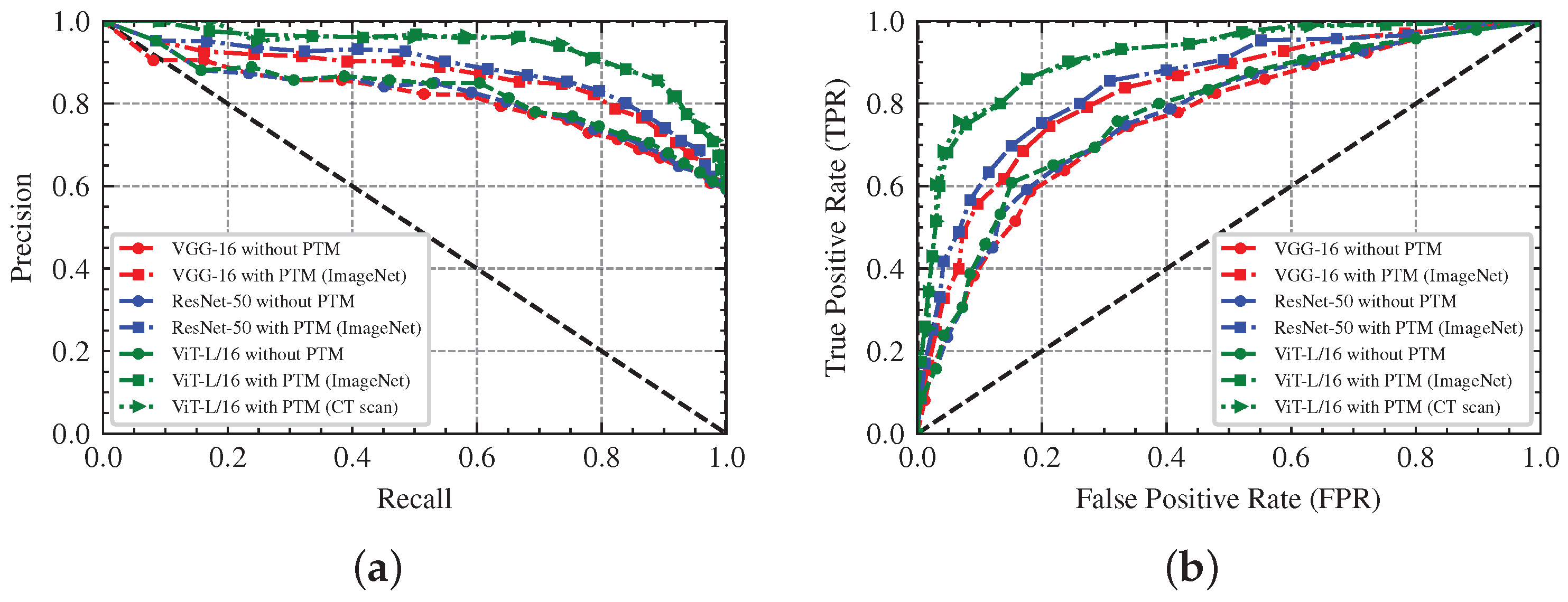
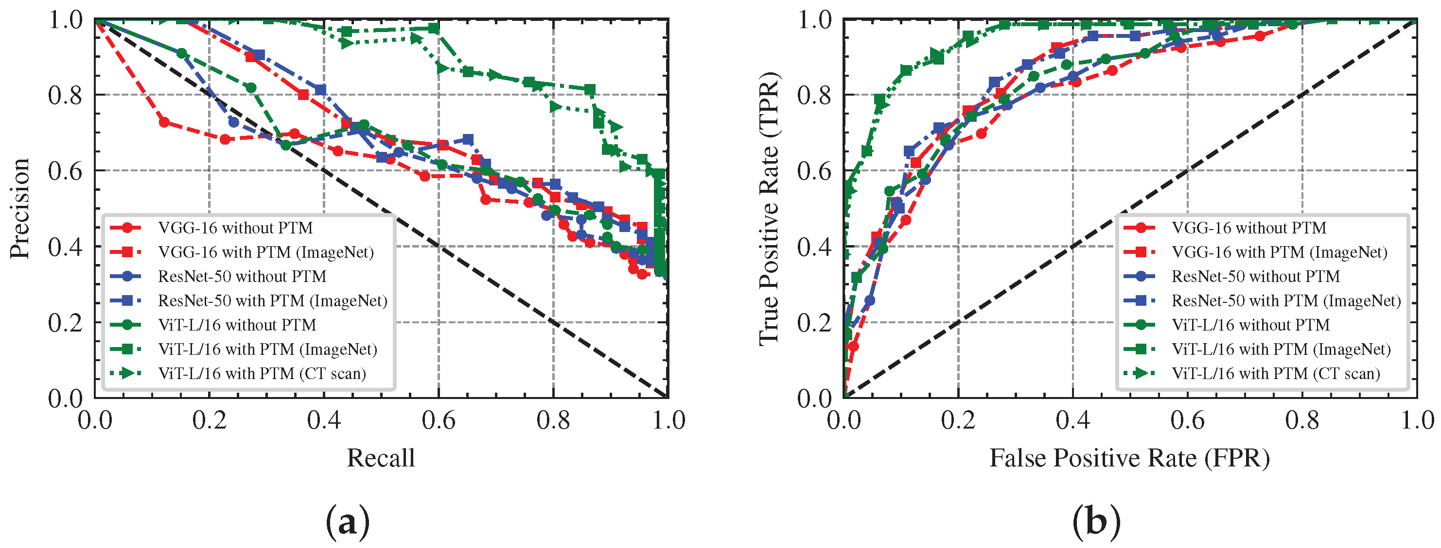
First, we performed experiments on the two federated learning tasks for predicting COVID-19 positive and severe separately to evaluate the performance of the pre-trained models. In the experiments, we used the ViT-L/16 architecture of the vision transformer neural network to build the deep learning models, and adopted two pre-trained model weights [57]. One of them was pre-trained on the ImageNet-22k dataset using iBOT [58] and fine-tuned on 165k CT slices (4000 patients from 7 public datasets) for 35 epochs, and the other was also pre-trained on the ImageNet-22k dataset but not fine-tuned. For comparison, we also built two classical convolutional neural network models, VGG-16 [59] and ResNet-50 [60], which were also pre-trained on the ImageNet-1k dataset. Under the federated learning settings, we tested the performance of the global model for using the VGG-16, ResNet-50 and ViT-L/16 models (with or without pre-trained model weights), respectively. The final test results for these models are shown in

Table 7. Comparison of Seven Models with or without Pre-Trained Model Weights.

Task	Model	Accuracy	Precision	Recall	${\mathit{F}}_1$-Score	FPR	AUC	Specificity
T${}_1$	A	0.7049	0.7174	0.8212	0.7658	0.4606	0.7606	0.5394
	B	0.7699	0.7826	0.8425	0.8114	0.3333	0.8310	0.6667
	C	0.7149	0.7265	0.8255	0.7729	0.4424	0.7721	0.5576
	D	0.7774	0.7851	0.8553	0.8187	0.3333	0.8481	0.6667
	E	0.7074	0.7122	0.8425	0.7719	0.4849	0.7810	0.5151
	F	0.8450	0.8777	0.8553	0.8663	0.1697	0.9158	0.8303
	G	0.8500	0.8691	0.8765	0.8728	0.1879	0.9162	0.8121
T${}_2$	A	0.7344	0.5106	0.7272	0.6000	0.2629	0.8075	0.7371
	B	0.7717	0.5617	0.7575	0.6451	0.2229	0.8630	0.7771
	C	0.7012	0.4741	0.8333	0.6043	0.3486	0.8260	0.6514
	D	0.7593	0.5392	0.8333	0.6547	0.2686	0.8621	0.7314
	E	0.7095	0.4830	0.8636	0.6195	0.3486	0.8400	0.6514
	F	0.8464	0.6629	0.8939	0.7612	0.1714	0.9531	0.8286
	G	0.8506	0.6666	0.9090	0.7690	0.1714	0.9514	0.8286

T${}_{\mathbf{1}}$: Positive Prediction task. T${}_{\mathbf{2}}$: Severe Prediction task. A: VGG-16 model without pre-trained weights. B: VGG-16 model with pre-trained weights trained on the ImageNet-1k dataset. C: ResNet-50 model without pre-trained weights. D: ResNet-50 model with pre-trained weights trained on the ImageNet-1k dataset. E: ViT-L/16 without pre-trained weights. F: ViT-L/16 with pre-trained weights trained on the ImageNet-22k dataset. G: ViT-L/16 with pre-trained weights trained on the ImageNet-22k dataset and fine-tuned with 165k CT slices. Note: Recall = TPR = Sensitivity.

, including Accuracy, Precision, Recall, and other metrics. As can be seen from the results, using the pre-trained model weights to train models can bring a higher performance improvement than not using the pre-trained model weights. Meanwhile, the ViT-L/16 models with pre-trained model weights achieve a better performance than the VGG-16 and ResNet-50 models. In addition, the fine-tuned ViT-L/16 model has a certain performance improvement.

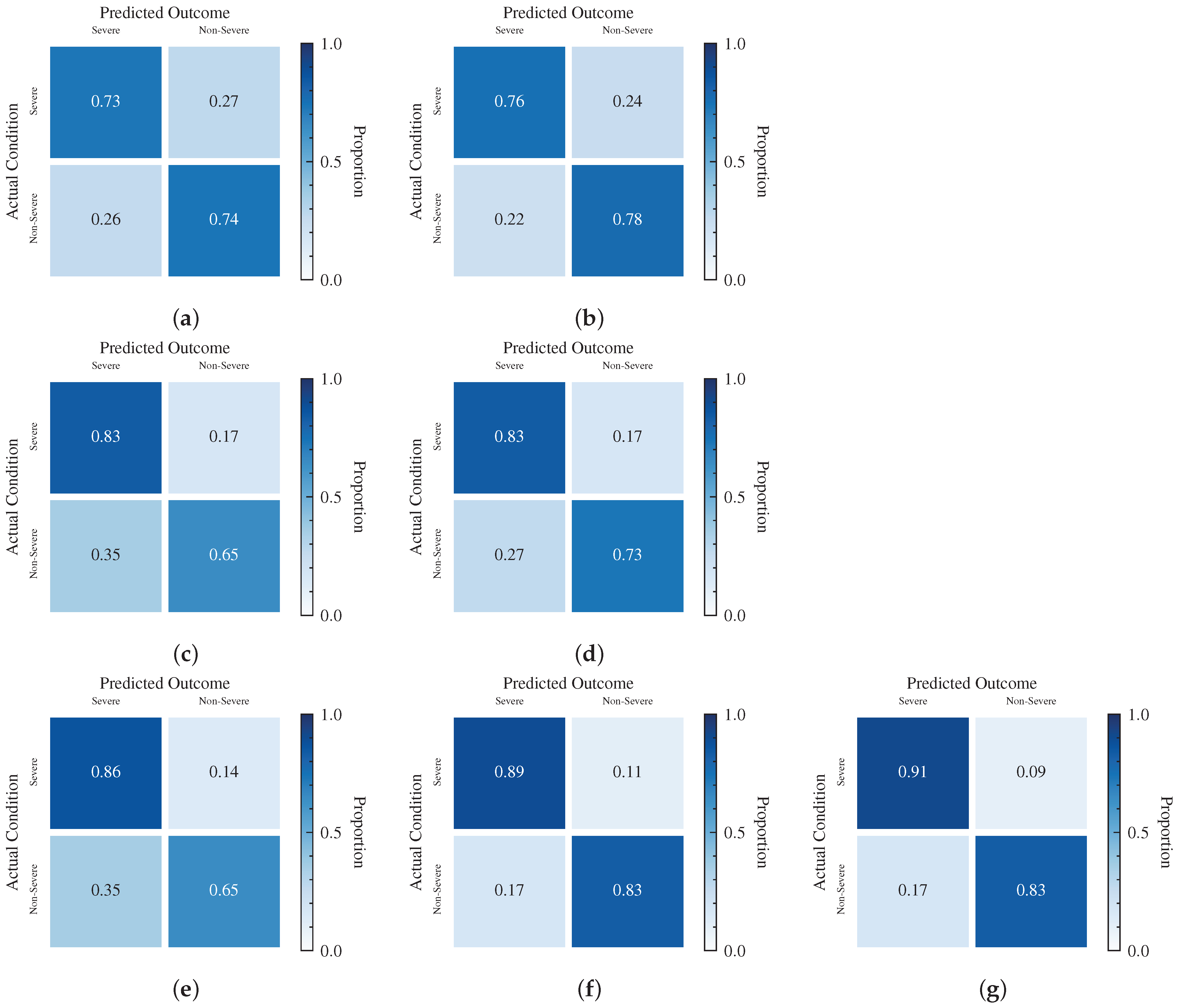
Based on the experimental data, we also draw the Precision-Recall (PR) curve, the receiver operating characteristic (ROC) curve and the confusion matrix of the seven models. The PR curve represents the relationship between Precision and Recall under different classification thresholds, and a model with perfect performance has the PR curve through coordinates $(0,1)$, which consists of a segment with $y=1,x\in [0,1]$ and a segment with $x=1,y\in [0,1]$. The ROC curve describes the relationship between Precision and Recall at various classification thresholds and it goes through points $(0,0)$ and $(1,1)$. Furthermore, the ROC curve of a perfect model consists of two segments, $x=10,y\in [0,1]$ and $y=1,x\in [0,1]$, which goes through point $(0,1)$. The AUC represents the area between the entire ROC curve from $(0,0)$ to $(1,1)$ and the X-axis, which is shown in Table 7. The confusion matrix gives the proportion of different predictions, TP, FN, FP and TN. The Figure 6 and Figure 7 are the PR curves, the ROC curves, and the confusion matrices of these models for positive prediction, while the Figure 8 and Figure 9 are the severe prediction. We can similarly conclude that the ViT-L/16 model with pre-trained model weights has the best performance for both positive and severe prediction.

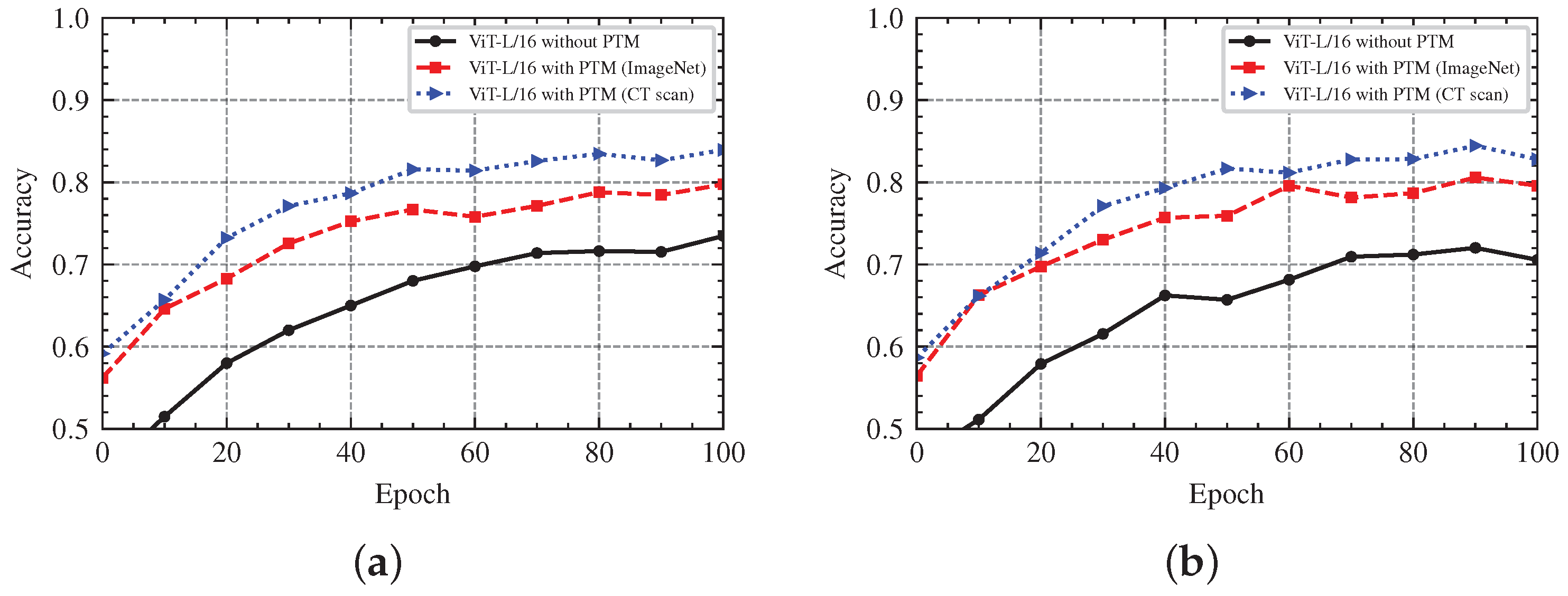
In addition, we also compare the accuracy trends of ViT-L/16 models with or without pre-trained model weights. After 100 epochs of global training, the accuracy of the global model for the ViT-L/16 models is shown in Figure 10. From the accuracy results of these models, we can conclude that the training model with pre-trained model weights has a faster convergence speed and a better model accuracy than training a new model from scratch, both in positive prediction and severity prediction.

6.3.2. Effectiveness of Differential Privacy

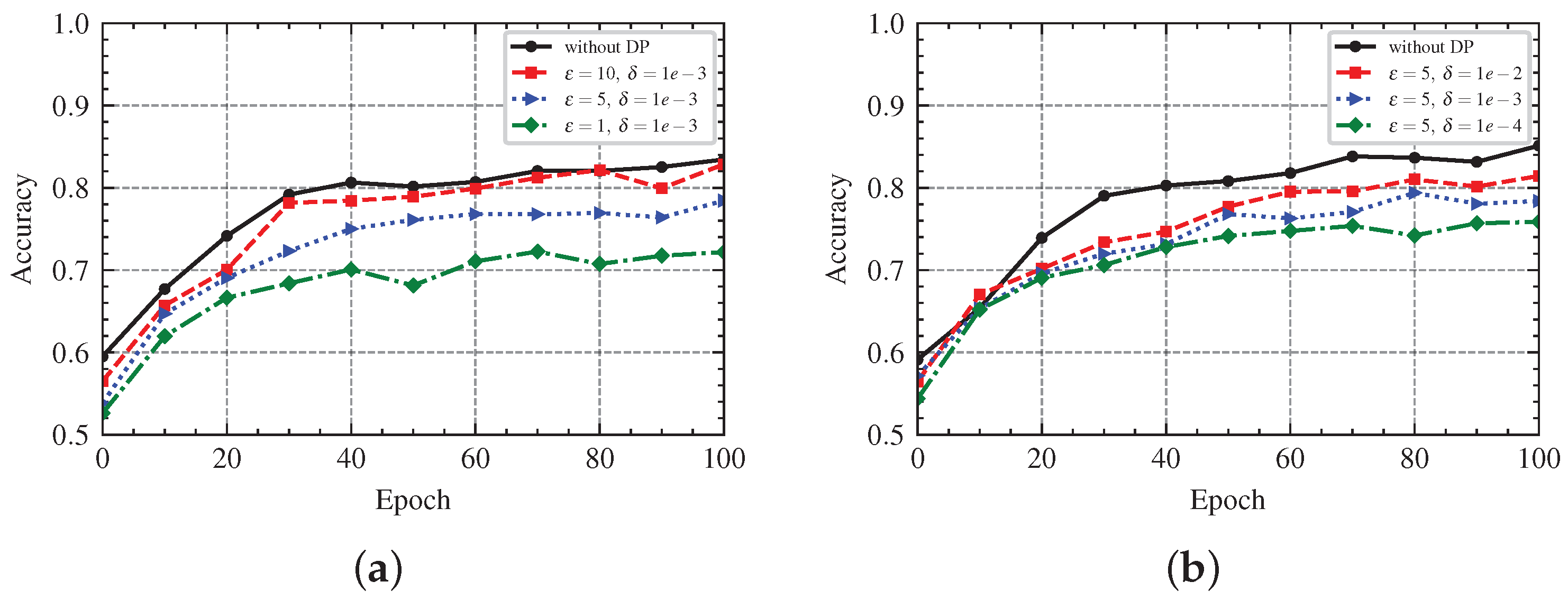
Next, we inspected the setting of the differential privacy mechanism. We guarantee $(ϵ,\delta )$-differential privacy by adding Gaussian noise to the gradients, while the Gaussian noise is confirmed by C and z, where C is the gradient clipping coefficient, which is also the $L2$ sensitivity upper bound of the gradient, and the privacy loss is only related to the noise multiplier z, which is determined by $ϵ$ and $\delta$. The privacy parameter $ϵ$ represents the privacy budget and $\delta$ is the relaxation term for differential privacy. We try to observe the influence of z under different combinations of $(ϵ,\delta )$ on the accuracy of the model. The result in Figure 11 shows that, when keeping the differential privacy relaxation term constant, the model accuracy decreases as $ϵ$ decreases, which indicates that more noise is added to the model and a high privacy protection strength is obtained. When keeping the privacy budget constant, the model accuracy decreases as $ϵ$ decreases, but the model still has a decent accuracy. It is common to set $ϵ$ to a small constant (lower values indicate tighter differential privacy conditions), and it is recommended to set $\delta$ to be less than the inverse of the size of the training dataset. It is easier to take $z=1$, so we use the combination $(ϵ=5,\delta =0.001)$ to achieve differential privacy.

6.3.3. Robustness of Byzantine Aggregation

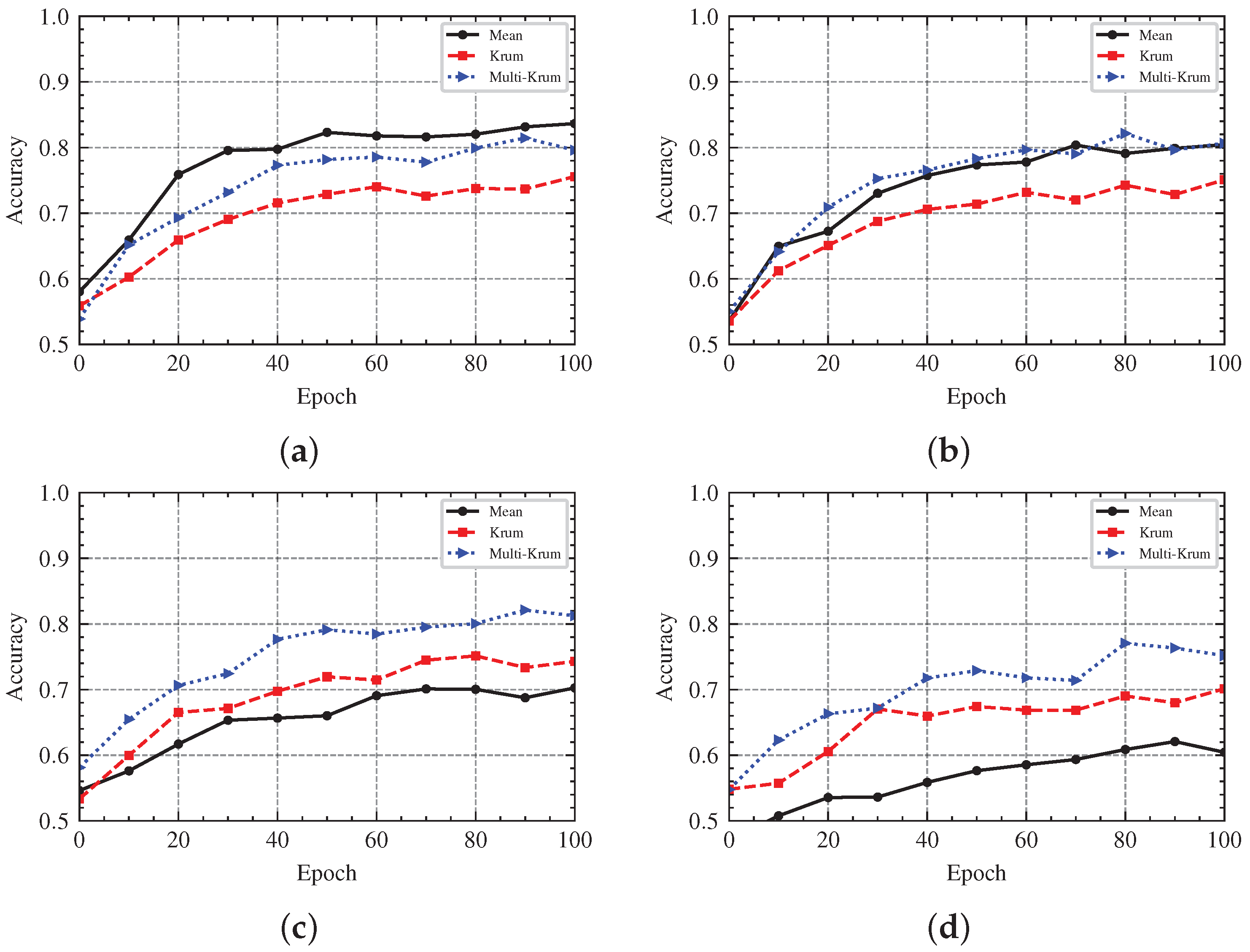
In the federated learning aggregation phase of our scheme, we consider a Byzantine fault-tolerant scenario to achieve Byzantine robust federated learning. We set $n=10$ clients to perform the training task, of which f clients are malicious (i.e., Byzantine nodes), where the data of the clients are independent and identically distributed. We performed perturbations on the data for Byzantine clients, such as label inversion, who submitted malicious models to the server to launch a poisoning attack on the aggregation process. Our goal is to filter out malicious models through appropriate strategies to prevent them from poisoning the global model under the premise that malicious clients are involved. We chose to use the Multi-Krum algorithm, a Byzantine fault-tolerant machine learning algorithm based on Euclidean distance, which is able to guarantee global model robustness in $2f+2<n$ cases. We contrast the Multi-Krum algorithm with two aggregation rules, Krum and Mean, in our experiments, where Multi-Krum selects $m=n-f$ models for aggregation. We set the number of malicious clients as $f=0$, $f=1$, $f=3,$ and $f=5$, respectively, to compare the accuracy changes of the global model under different proportions of malicious clients, respectively. In Figure 12, we find that when the proportions of malicious clients are 0%, 10%, and 30%, the global model accuracy of the two aggregation algorithms, Multi-Krum and Krum, hardly shows any change, while the accuracy of the mean aggregation rule decreases with the increase of the number of malicious clients. This is because Multi-Krum and Krum filter the malicious models and only aggregate the models submitted by honest clients under the condition that $2f+2<n$ is satisfied, but the mean aggregates the models submitted by all clients. When the proportion of malicious clients is 50%, the condition $2f+2<n$ is not satisfied, so Multi-Krum and Krum algorithms cannot avoid poisoning attacks, and the accuracy will be reduced.

6.3.4. Efficiency of Homomorphic Encryption

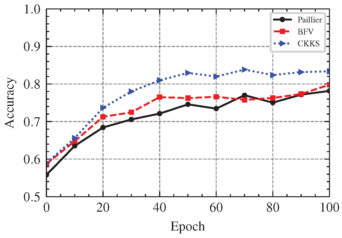
In order to protect user’s data security and prevent inferential attacks from servers, we replace the central server of federated learning with two honest but curious servers, and assume that there is no collusion between them. Homomorphic encryption algorithm provides the ability to perform operations on ciphertext. It can make good use of the server for computing without providing plaintext data to the server. Therefore, we use a homomorphic encryption scheme to encrypt the calculation process, so that the aggregation server can execute the aggregation algorithm on the ciphertext model. Common homomorphic encryption schemes include the partially homomorphic encryption Paillier algorithm [42], full-homomorphic encryption BFV algorithm, and CKKS algorithm. The Paillier algorithm supports homomorphic addition and scalar multiplication, and can be used to implement aggregation algorithms. The BFV and CKKS algorithms not only support homomorphic addition operation, but also provide homomorphic multiplication, rotation, and other operations, and CKKS supports homomorphic operation at the level of floating-point numbers and complex numbers.

Table 8. The Storage and Time Cost of Homomorphic Encryption Schemes.

Plaintext Size	Scheme	Ciphertext Size	Encrypt Time (s)	Decrypt Time (s)	Aggregate Time (s)
1024 (8 KB)	Paillier	372B	43.08	12.70	48.90
	BFV	524KB	0.06	0.04	0.15
	CKKS	1MB	0.17	0.06	0.24

lists the storage and time costs of these three homomorphic encryption schemes in encrypting a vector data. Combined with Figure 13, we find that, although the ciphertext size after encryption by Paillier algorithm is small, its time cost is large. In contrast, both the BFV and CKKS schemes have much less time overhead in encryption, decryption, and aggregation calculations than the Paillier schemes, and they support more operations. As can be seen from Figure 14, the accuracy of the global model under the CKKS scheme encryption is higher than the other two, because both the Paillier and the BFV scheme operate in the integer range, and for floating-point numbers, scaling and rounding are required, which introduce inaccuracy. Therefore, using the CKKS algorithm as the homomorphic encryption scheme not only provides efficient operation speed, but also ensures that the accuracy of global model is not affected.

6.3.5. Performance of Blockchain Storage

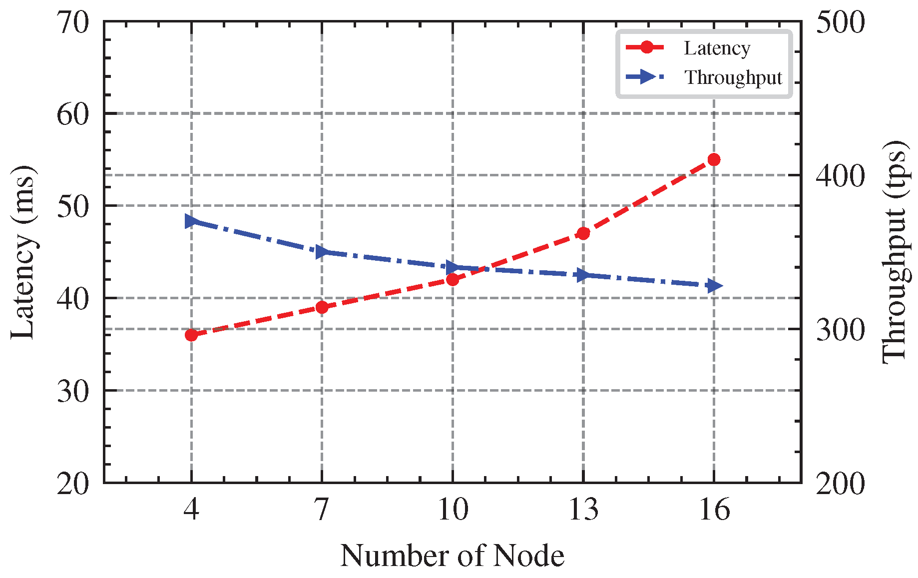
Finally, we use Hyperledger Fabric as the blockchain platform for our experiments to provide distributed storage capabilities, while we integrate the SmartBFT consensus algorithm for Hyperledger Fabric to make up for its lack of support for BFT-like consensus protocols. Through the SmartBFL algorithm, it can ensure that the local model trained by the clients and the global model aggregated by the servers are correctly recorded on the blockchain for traceability anytime, and avoid single points of failure and malicious attacks, so as to achieve the goal of enhancing robustness. We used a docker to build a blockchain network in the local environment and test its performance (e.g., latency and throughput). Specifically, we set the transaction size to 1024 bytes and configure the Hyperledger Fabric with BatchTimeout = 10 s, MaxMessageCount = 100, AbsoluteMaxBytes = 10 MB and PreferredMaxBytes = 512 KB. We conducted the experiment of the number of consensus nodes with $n=4,7,10,13,16$, respectively, and they all satisfied $3f+1=n$ Byzantine fault-tolerant security corresponding with $f=1,2,3,4,5$, respectively. The results in Figure 15 show that SmartBFT provides a high throughput and low latency while providing $3f+1=n$ robustness.

7. Conclusions and Future Work

In this paper, we propose an efficient trusted federated learning scheme for COVID-19 detection, which is resistant to Byzantine attacks and supports privacy protection. We use pre-trained models to accelerate the training process, improve the detection accuracy, and reduce the communication overhead. To improve the robustness and privacy, we use CKKS fully homomorphic encryption to implement the Multi-Krum secure aggregation scheme, and introduce differential privacy to enhance privacy. In addition, we implement a blockchain with Hyperledger Fabric to promote the transparency of the training process, while integrating SmartBFL consensus to further improve the robustness. Lastly, we evaluate our scheme with a real dataset, and the results show that our scheme is robust with higher detection accuracy and shorter training time.

In future work, we will strive to improve our scheme by conducting more additional experiments to further improve the efficiency and accuracy, and enhance the robustness and privacy. In addition, we also plan to extend our scheme to different medical fields, which will be greatly meaningful.

References

1. Bedford, J.; Enria, D.; Giesecke, J.; Heymann, D.L.; Ihekweazu, C.; Kobinger, G.; Lane, H.C.; Memish, Z.; don Oh, M.; Sall, A.A.; et al. COVID-19: Towards controlling of a pandemic. Lancet 2020, 395, 1015–1018. [Google Scholar] [CrossRef]
2. Li, M. Chest CT features and their role in COVID-19. Radiol. Infect. Dis. 2020, 7, 51–54. [Google Scholar] [CrossRef]
3. Zhao, J.Y.; Yan, J.Y.; Qu, J.M. Interpretations of “Diagnosis and Treatment Protocol for Novel Coronavirus Pneumonia (Trial Version 7)”. Chin. Med J. 2020, 133, 1347–1349. [Google Scholar] [CrossRef]
4. Wang, J.; Liu, J.; Wang, Y.; Liu, W.; Chen, X.; Sun, C.; Shen, X.; Wang, Q.; Wu, Y.; Liang, W.; et al. Dynamic changes of chest CT imaging in patients with COVID-19. J. Zhejiang Univ. Med Sci. 2020, 49, 191–197. [Google Scholar] [CrossRef]
5. Song, Y.; Zheng, S.; Li, L.; Zhang, X.; Zhang, X.; Huang, Z.; Chen, J.; Wang, R.; Zhao, H.; Chong, Y.; et al. Deep Learning Enables Accurate Diagnosis of Novel Coronavirus (COVID-19) With CT Images. IEEE/ACM Trans. Comput. Biol. Bioinform. 2021, 18, 2775–2780. [Google Scholar] [CrossRef]
6. Ozturk, T.; Talo, M.; Yildirim, E.A.; Baloglu, U.B.; Yildirim, O.; Acharya, U.R. Automated detection of COVID-19 cases using deep neural networks with X-ray images. Comput. Biol. Med. 2020, 121, 103792. [Google Scholar] [CrossRef]
7. Tai, Y.; Gao, B.; Li, Q.; Yu, Z.; Zhu, C.; Chang, V. Trustworthy and Intelligent COVID-19 Diagnostic IoMT Through XR and Deep-Learning-Based Clinic Data Access. IEEE Internet Things J. 2021, 8, 15965–15976. [Google Scholar] [CrossRef]
8. Voigt, P.; von dem Bussche, A. The EU General Data Protection Regulation (GDPR); Springer International Publishing: Cham, Switzerland, 2017. [Google Scholar] [CrossRef]
9. Yang, J.J.; Li, J.Q.; Niu, Y. A hybrid solution for privacy preserving medical data sharing in the cloud environment. Future Gener. Comput. Syst. 2015, 43–44, 74–86. [Google Scholar] [CrossRef]
10. Zhao, Y.; Zhao, J.; Jiang, L.; Tan, R.; Niyato, D.; Li, Z.; Lyu, L.; Liu, Y. Privacy-Preserving Blockchain-Based Federated Learning for IoT Devices. IEEE Internet Things J. 2021, 8, 1817–1829. [Google Scholar] [CrossRef]
11. Wang, R.; Lai, J.; Zhang, Z.; Li, X.; Vijayakumar, P.; Karuppiah, M. Privacy-Preserving Federated Learning for Internet of Medical Things under Edge Computing. IEEE J. Biomed. Health Inform. 2022, 27, 854–865. [Google Scholar] [CrossRef]
12. Treleaven, P.; Smietanka, M.; Pithadia, H. Federated Learning: The Pioneering Distributed Machine Learning and Privacy-Preserving Data Technology. Computer 2022, 55, 20–29. [Google Scholar] [CrossRef]
13. Yang, Q.; Liu, Y.; Chen, T.; Tong, Y. Federated Machine Learning. ACM Trans. Intell. Syst. Technol. 2019, 10, 1–19. [Google Scholar] [CrossRef]
14. Kairouz, P.; McMahan, H.B.; Avent, B.; Bellet, A.; Bennis, M.; Bhagoji, A.N.; Bonawitz, K.; Charles, Z.; Cormode, G.; Cummings, R.; et al. Advances and Open Problems in Federated Learning. arXiv 2019, arXiv:1912.04977. [Google Scholar]
15. Ronneberger, O.; Fischer, P.; Brox, T. U-Net: Convolutional Networks for Biomedical Image Segmentation. In Proceedings of the Medical Image Computing and Computer-Assisted Intervention—MICCAI 2015, Munich, Germany, 5–9 October 2015; pp. 234–241. [Google Scholar] [CrossRef]
16. Badrinarayanan, V.; Kendall, A.; Cipolla, R. SegNet: A Deep Convolutional Encoder-Decoder Architecture for Image Segmentation. IEEE Trans. Pattern Anal. Mach. Intell. 2017, 39, 2481–2495. [Google Scholar] [CrossRef]
17. Dosovitskiy, A.; Beyer, L.; Kolesnikov, A.; Weissenborn, D.; Zhai, X.; Unterthiner, T.; Dehghani, M.; Minderer, M.; Heigold, G.; Gelly, S.; et al. An Image is Worth 16x16 Words: Transformers for Image Recognition at Scale. arXiv 2020, arXiv:2010.11929. [Google Scholar]
18. Rajpurkar, P.; Irvin, J.; Zhu, K.; Yang, B.; Mehta, H.; Duan, T.; Ding, D.; Bagul, A.; Langlotz, C.; Shpanskaya, K.; et al. CheXNet: Radiologist-Level Pneumonia Detection on Chest X-Rays with Deep Learning. arXiv 2017, arXiv:1711.05225. [Google Scholar]
19. Habib, N.; Hasan, M.M.; Reza, M.M.; Rahman, M.M. Ensemble of CheXNet and VGG-19 Feature Extractor with Random Forest Classifier for Pediatric Pneumonia Detection. SN Comput. Sci. 2020, 1, 359. [Google Scholar] [CrossRef]
20. Lee, E.H.; Zheng, J.; Colak, E.; Mohammadzadeh, M.; Houshmand, G.; Bevins, N.; Kitamura, F.; Altinmakas, E.; Reis, E.P.; Kim, J.K.; et al. Deep COVID DeteCT: An international experience on COVID-19 lung detection and prognosis using chest CT. Npj Digit. Med. 2021, 4, 11. [Google Scholar] [CrossRef]
21. Al-Waisy, A.S.; Al-Fahdawi, S.; Mohammed, M.A.; Abdulkareem, K.H.; Mostafa, S.A.; Maashi, M.S.; Arif, M.; Garcia-Zapirain, B. COVID-CheXNet: Hybrid deep learning framework for identifying COVID-19 virus in chest X-rays images. Soft Comput. 2023, 27, 2657–2672. [Google Scholar] [CrossRef]
22. Gozes, O.; Frid-Adar, M.; Greenspan, H.; Browning, P.D.; Zhang, H.; Ji, W.; Bernheim, A.; Siegel, E. Rapid AI Development Cycle for the Coronavirus (COVID-19) Pandemic: Initial Results for Automated Detection & Patient Monitoring using Deep Learning CT Image Analysis. arXiv 2020, arXiv:2003.05037. [Google Scholar]
23. Gupta, R.K.; Kunhare, N.; Pathik, N.; Pathik, B. An AI-enabled pre-trained model-based Covid detection model using chest X-ray images. Multimed. Tools Appl. 2022, 81, 37351–37377. [Google Scholar] [CrossRef]
24. Xiao, B.; Yang, Z.; Qiu, X.; Xiao, J.; Wang, G.; Zeng, W.; Li, W.; Nian, Y.; Chen, W. PAM-DenseNet: A Deep Convolutional Neural Network for Computer-Aided COVID-19 Diagnosis. IEEE Trans. Cybern. 2022, 52, 12163–12174. [Google Scholar] [CrossRef]
25. Kumar, R.; Khan, A.A.; Kumar, J.; Zakria; Golilarz, N.A.; Zhang, S.; Ting, Y.; Zheng, C.; Wang, W. Blockchain-Federated-Learning and Deep Learning Models for COVID-19 Detection Using CT Imaging. IEEE Sens. J. 2021, 21, 16301–16314. [Google Scholar] [CrossRef]
26. Yang, D.; Xu, Z.; Li, W.; Myronenko, A.; Roth, H.R.; Harmon, S.; Xu, S.; Turkbey, B.; Turkbey, E.; Wang, X.; et al. Federated semi-supervised learning for COVID region segmentation in chest CT using multi-national data from China, Italy, Japan. Med. Image Anal. 2021, 70, 101992. [Google Scholar] [CrossRef]
27. Dayan, I.; Roth, H.R.; Zhong, A.; Harouni, A.; Gentili, A.; Abidin, A.Z.; Liu, A.; Costa, A.B.; Wood, B.J.; Tsai, C.S.; et al. Federated learning for predicting clinical outcomes in patients with COVID-19. Nat. Med. 2021, 27, 1735–1743. [Google Scholar] [CrossRef]
28. Kandati, D.R.; Gadekallu, T.R. Genetic Clustered Federated Learning for COVID-19 Detection. Electronics 2022, 11, 2714. [Google Scholar] [CrossRef]
29. Yang, Q.; Zhang, J.; Hao, W.; Spell, G.P.; Carin, L. FLOP: Federated Learning on Medical Datasets using Partial Networks. ACM 2021, 8, 3845–3853. [Google Scholar] [CrossRef]
30. McMahan, H.B.; Moore, E.; Ramage, D.; Hampson, S.; y Arcas, B.A. Communication-Efficient Learning of Deep Networks from Decentralized Data. arXiv 2016, arXiv:1602.05629. [Google Scholar]
31. Blanchard, P.; Mhamdi, E.M.E.; Guerraoui, R.; Stainer, J. Byzantine-Tolerant Machine Learning. arXiv 2017, arXiv:1703.02757. [Google Scholar]
32. Yin, D.; Chen, Y.; Ramchandran, K.; Bartlett, P. Byzantine-Robust Distributed Learning: Towards Optimal Statistical Rates. arXiv 2018, arXiv:1803.01498. [Google Scholar]
33. Truex, S.; Baracaldo, N.; Anwar, A.; Steinke, T.; Ludwig, H.; Zhang, R.; Zhou, Y. A Hybrid Approach to Privacy-Preserving Federated Learning. In Proceedings of the 12th ACM Workshop on Artificial Intelligence and Security, London, UK, 15 November 2019; pp. 1–11. [Google Scholar] [CrossRef]
34. Wibawa, F.; Catak, F.O.; Kuzlu, M.; Sarp, S.; Cali, U. Homomorphic Encryption and Federated Learning based Privacy-Preserving CNN Training: COVID-19 Detection Use-Case. In Proceedings of the European Interdisciplinary Cybersecurity Conference (EICC), Barcelona, Spain, 15–16 June 2022; pp. 85–90. [Google Scholar] [CrossRef]
35. Miao, Y.; Liu, Z.; Li, H.; Choo, K.K.R.; Deng, R.H. Privacy-Preserving Byzantine-Robust Federated Learning via Blockchain Systems. IEEE Trans. Inf. Forensics Secur. 2022, 17, 2848–2861. [Google Scholar] [CrossRef]
36. Qu, Y.; Gao, L.; Luan, T.H.; Xiang, Y.; Yu, S.; Li, B.; Zheng, G. Decentralized Privacy Using Blockchain-Enabled Federated Learning in Fog Computing. IEEE Internet Things J. 2020, 7, 5171–5183. [Google Scholar] [CrossRef]
37. Shayan, M.; Fung, C.; Yoon, C.J.M.; Beschastnikh, I. Biscotti: A Blockchain System for Private and Secure Federated Learning. IEEE Trans. Parallel Distrib. Syst. 2021, 32, 1513–1525. [Google Scholar] [CrossRef]
38. Nguyen, D.C.; Ding, M.; Pathirana, P.N.; Seneviratne, A.; Zomaya, A.Y. Federated Learning for COVID-19 Detection With Generative Adversarial Networks in Edge Cloud Computing. IEEE Internet Things J. 2022, 9, 10257–10271. [Google Scholar] [CrossRef]
39. Yang, Z.; Shi, Y.; Zhou, Y.; Wang, Z.; Yang, K. Trustworthy Federated Learning via Blockchain. IEEE Internet Things J. 2023, 10, 92–109. [Google Scholar] [CrossRef]
40. Islam, A.; Amin, A.A.; Shin, S.Y. FBI: A Federated Learning-Based Blockchain-Embedded Data Accumulation Scheme Using Drones for Internet of Things. IEEE Wirel. Commun. Lett. 2022, 11, 972–976. [Google Scholar] [CrossRef]
41. Yoosuf, M.S.; Muralidharan, C.; Shitharth, S.; Alghamdi, M.; Maray, M.; Rabie, O.B.J. FogDedupe: A Fog-Centric Deduplication Approach Using Multi-Key Homomorphic Encryption Technique. J. Sensors 2022, 2022, 6759875. [Google Scholar] [CrossRef]
42. Paillier, P. Public-Key Cryptosystems Based on Composite Degree Residuosity Classes; Springer: Berlin/Heidelberg, Germany, 1999; pp. 223–238. [Google Scholar] [CrossRef]
43. Brakerski, Z.; Gentry, C.; Vaikuntanathan, V. Fully Homomorphic Encryption without Bootstrapping. Cryptology ePrint Archive, Paper 2011/277. 2011. Available online: https://eprint.iacr.org/2011/277 (accessed on 1 June 2022).
44. Fan, J.; Vercauteren, F. Somewhat Practical Fully Homomorphic Encryption. Cryptology ePrint Archive, Paper 2012/144. 2012. Available online: https://eprint.iacr.org/2012/144 (accessed on 1 June 2022).
45. Cheon, J.H.; Kim, A.; Kim, M.; Song, Y. Homomorphic Encryption for Arithmetic of Approximate Numbers. In Proceedings of the Advances in Cryptology–ASIACRYPT 2017: 23rd International Conference on the Theory and Applications of Cryptology and Information Security, Hong Kong, China, 3–7 December 2017; pp. 409–437. [Google Scholar] [CrossRef]
46. Ghadimi, S.; Lan, G. Stochastic First- and Zeroth-Order Methods for Nonconvex Stochastic Programming. SIAM J. Optim. 2013, 23, 2341–2368. [Google Scholar] [CrossRef]
47. Revel, M.P.; Boussouar, S.; de Margerie-Mellon, C.; Saab, I.; Lapotre, T.; Mompoint, D.; Chassagnon, G.; Milon, A.; Lederlin, M.; Bennani, S.; et al. Study of Thoracic CT in COVID-19: The STOIC Project. Radiology 2021, 301, E361–E370. [Google Scholar] [CrossRef]
48. STOIC2021 Training—Registry of Open Data on AWS. Available online: https://registry.opendata.aws/stoic2021-training/ (accessed on 30 September 2022).
49. Paszke, A.; Gross, S.; Massa, F.; Lerer, A.; Bradbury, J.; Chanan, G.; Killeen, T.; Lin, Z.; Gimelshein, N.; Antiga, L.; et al. PyTorch: An Imperative Style, High-Performance Deep Learning Library. In Proceedings of the Advances in Neural Information Processing Systems 32, Vancouver, BC, Canada, 8–14 December 2019; Wallach, H., Larochelle, H., Beygelzimer, A., d’Alché Buc, F., Fox, E., Garnett, R., Eds.; Curran Associates, Inc.: New York, NY, USA, 2019; pp. 8024–8035. [Google Scholar]
50. Yousefpour, A.; Shilov, I.; Sablayrolles, A.; Testuggine, D.; Prasad, K.; Malek, M.; Nguyen, J.; Ghosh, S.; Bharadwaj, A.; Zhao, J.; et al. Opacus: User-Friendly Differential Privacy Library in PyTorch. arXiv 2021, arXiv:2109.12298. [Google Scholar]
51. Ibarrondo, A.; Viand, A. Pyfhel: Python for homomorphic encryption libraries. ACM 2021, 11, 11–16. [Google Scholar] [CrossRef]
52. Androulaki, E.; Barger, A.; Bortnikov, V.; Cachin, C.; Christidis, K.; Caro, A.D.; Enyeart, D.; Ferris, C.; Laventman, G.; Manevich, Y.; et al. Hyperledger fabric: A distributed operating system for permissioned blockchains. ACM 2018, 4, 1–15. [Google Scholar] [CrossRef]
53. Barger, A.; Manevich, Y.; Meir, H.; Tock, Y. A Byzantine Fault-Tolerant Consensus Library for Hyperledger Fabric. IEEE 2021, 5, 1–9. [Google Scholar] [CrossRef]
54. Manoharan, H.; Haleem, S.L.A.; Shitharth, S.; Kshirsagar, P.R.; Tirth, V.; Thangamani, M.; Chandan, R.R. A machine learning algorithm for classification of mental tasks. Comput. Electr. Eng. 2022, 99, 107785. [Google Scholar] [CrossRef]
55. Kshirsagar, P.R.; Manoharan, H.; Shitharth, S.; Alshareef, A.M.; Albishry, N.; Balachandran, P.K. Deep Learning Approaches for Prognosis of Automated Skin Disease. Life 2022, 12, 426. [Google Scholar] [CrossRef]
56. Shitharth, S.; Winston, D.P. Comparison of PRC based RVM classification versus SVM classification in SCADA network. J. Electr. Eng. 2017, 17, 318–331. [Google Scholar]
57. Jégou, S. Weights of Two ViT-L Models. 2022. Available online: https://zenodo.org/record/6547999 (accessed on 30 September 2022).
58. Zhou, J.; Wei, C.; Wang, H.; Shen, W.; Xie, C.; Yuille, A.; Kong, T. iBOT: Image BERT Pre-Training with Online Tokenizer. arXiv 2021, arXiv:2111.07832. [Google Scholar]
59. Simonyan, K.; Zisserman, A. Very Deep Convolutional Networks for Large-Scale Image Recognition. arXiv 2014, arXiv:1409.1556. [Google Scholar]
60. He, K.; Zhang, X.; Ren, S.; Sun, J. Deep Residual Learning for Image Recognition. IEEE 2016, 6, 770–778. [Google Scholar] [CrossRef]
Figure 1. System Architecture.
Electronics 12 02068 g001
Figure 2. The Standard FL Model.
Electronics 12 02068 g002
Figure 3. The Pre-Trained ViT Model.
Electronics 12 02068 g003
Figure 4. Distribution of Sex in the Dataset.
Electronics 12 02068 g004
Figure 5. Distribution of Age in the Dataset.
Electronics 12 02068 g005
Figure 6. PR and ROC Curve of Seven Models in Positive Prediction: (a) PR Curve; (b) ROC Curve.
Electronics 12 02068 g006
Figure 7. Confusion Matrix of Seven Models in Positive Prediction. (a) VGG-16 Model without PTM Weights. (b) VGG-16 Model with PTM Weights (ImageNet). (c) ResNet-50 Model without PTM Weights. (d) ResNet-50 Model with PTM Weights (ImageNet). (e) ViT-L/16 Model without PTM Weights. (f) ViT-L/16 Model with PTM Weights (ImageNet). (g) ViT-L/16 Model with PTM Weights (CT scan).
Electronics 12 02068 g007
Figure 8. PR and ROC Curve of Seven Models in Severe Prediction: (a) PR Curve; (b) ROC Curve.
Electronics 12 02068 g008
Figure 9. Confusion Matrix of Seven Models in Severe Prediction. (a) VGG-16 Model without PTM Weights. (b) VGG-16 Model with PTM Weights (ImageNet). (c) ResNet-50 Model without PTM Weights. (d) ResNet-50 Model with PTM Weights (ImageNet). (e) ViT-L/16 Model without PTM Weights. (f) ViT-L/16 Model with PTM Weights (ImageNet). (g) ViT-L/16 Model with PTM Weights (CT scan).
Electronics 12 02068 g009
Figure 10. Federated Learning with Pre-Trained Models. (a) The Accuracy of Positive Prediction. (b) The Accuracy of Severe Prediction.
Electronics 12 02068 g010
Figure 11. Federated Learning with ( ϵ , δ ) -Differential Privacy. (a) The Accuracy at Different ϵ . (b) The Accuracy at Different δ .
Electronics 12 02068 g011
Figure 12. Federated Learning with BFT Aggregation Rule. (a) The Accuracy under 0% Malicious Clients. (b) The Accuracy under 10% Malicious Clients. (c) The Accuracy under 30% Malicious Clients. (d) The Accuracy under 50% Malicious Clients.
Electronics 12 02068 g012
Figure 13. The Time Cost of Different HE Schemes.
Electronics 12 02068 g013
Figure 14. The Accuracy of Different HE Schemes.
Electronics 12 02068 g014
Figure 15. Performance Evaluation of Blockchain Network.
Electronics 12 02068 g015