An Integrated Motion Planning Scheme for Safe Autonomous Vehicles in Highly Dynamic Environments

Abstract

This study proposes a new integrated approach to the motion control of autonomous vehicles, which differs from the conventional method of treating planning and tracking tasks as separate or hierarchical components. By means of the proposed approach we can reduce the side effects on the performance of autonomous vehicles under challenging driving circumstances. To this end, our approach processes both of the aforementioned tasks asynchronously and simultaneously utilizes a multi-threaded architecture to enhance control performance. Meanwhile, the behavior planning feature is integrated into the path-tracking module. Then, a linear parameter-varying model predictive control is deployed for trajectory tracking of autonomous vehicles and compared with the linear model predictive control method. Finally, the control performance of the proposed approach was evaluated through simulation trials on urban roads with placed obstacles. The outcomes revealed that the suggested framework satisfies the processing rate and high-precision criteria, while safely avoiding obstacles, indicating that it is a promising control strategy for real-world applications.

1. Introduction

With the rapid development of technology, the concepts of intelligent transportation systems and autonomous vehicles (AVs) are gradually becoming familiar to the public. The potential applications in AVs are being developed, tested, and commercialized globally [1,2]. Even though there have been successful implementations, it is quite obvious that many challenges remain for the techniques applied to AVs. The development of autonomous driving systems not only profoundly improves their operational accuracy and efficiency but also ensures the safety of passengers and pedestrians. In order to deploy an autonomous driving framework to improve the degree of AV autonomy, the general design of an autonomous driving system for the AV requires consideration of several aspects, such as sensor fusion, perception, decision making, and control [3,4]. In this work, the sensor fusion and perception modules are assumed to be working satisfactorily, since the main focus is on the development of planning and tracking control strategies for AVs.

In a fundamental context involving the appearance of obstacles on the road toward a defined goal, path planning determines the optimal path of the vehicle, while avoiding collisions. It can be further classified as global and local path planning with associated planning methods. Then, path tracking and execution ensure the vehicle follows the reference path with minimum errors. First of all, a global path is searched for and provided to the local planner. Many search-based algorithms, such as D* method, A* method and rapidly-exploring random trees, have been widely applied to motion planning, due to their high-computational efficiency [5,6,7,8,9,10]. They incorporate well-selected motion primitives and heuristics to significantly improve the planning process. In addition, several curve-based methods are employed to deal with limitations to smooth path generation, such as the following: Bezier [11], Spline [12], polynomial [13], optimization [14], and generation-selection [15].

In order to improve the maneuverability of the AV, a variety of local planning strategies have been proposed [16,17,18,19,20,21]. In [20], scholars designated obstacles with repulsive forces and obstacle-free areas with attractive forces by using potential field strategies. Intrinsically, obstacle avoidance algorithms predict the future vehicle position by considering constraints [21]. Other efficient local planning approaches generate multiple rollouts [22,23], i.e., running parallel to a reference path. Successively, these rollouts are leveraged by sampling and optimization. It is worth noting that path planning and tracking are essential to the operation, despite their functional and structural disparities. Thus, assorted control strategies have been proposed to achieve path-planning and path-tracking control. For example, the proportional-integral-radius and particle swarm optimization controllers were employed in [24]. Further, some scholars are devoted to the research of automatic cruise and automatic drive of engineering vehicles. More recent approaches take pedestrian factors into account to find safe paths [25]. The study in [26] examined a decision-making algorithm for executing the double lane change maneuver in dynamic situations. Additionally, the study in [27,28] discussed the utility of deep reinforcement learning on rough terrain vehicles. Nevertheless, it appeared to be ineffective for control purposes of real vehicles.

Alternatively, to bridge the gap between research and reality in the autonomous driving domain, various control strategies have been proposed to achieve accurate tracking performance. The model predictive control (MPC) approach is considered one of the most promising approaches, owing to its capability to systematically handle multiple constrained optimization problems. To achieve a high-performance trajectory control, a nonlinear MPC approach is employed for offline calculation of trajectory planning [29] and path tracking [30]. Aiming to handle the uncertainty term, several integrated MPC techniques are proposed to ensure tracking accuracy and smoothness, such as the MPC technique-based integrated control strategy [31], the linear parameter-varying system-based MPC technique (LPV–PMC) [32] and incorporating a gain-schedule robust control strategy [33]. In [34], the robust MPC approach with a finite time horizon was proposed. Recently, several studies have considered the tasks of motion planning and control together [35,36]. The target trajectory is obtained by the MPC technique in [35], and, meanwhile, an artificial potential is deployed in [36], wherein the MPC technique incorporates proportional-integral-derivative feedback to effectively follow the reference trajectory. Nonetheless, the presence of obstacles on the target trajectory may endanger decision accuracy, as well as system stability. Therefore, the deployment of an appropriate tracking controller is a crucial task.

Motivated by these developments, this paper develops an asynchronous framework for motion planning and path-tracking control for AVs, which can run simultaneously through multi-threading to improve the performance of the AV system. The proposed strategy structure is carried out with lightweight design and safety design in motion planning, and the initial state and kinematic models of the vehicle are considered. Moreover, the suggested framework was tested in a simulated environment with several obstacles and the results showed its effectiveness in smooth and quick responses. Meanwhile, the cost changes were analyzed in the process of motion planning, and the path-tracking effects of the adopted LPV–MPC and MPC control methods.

The remainder of the paper is organized as follows. Section 2 describes the proposed approach, including the motion planning and path tracking-based LPV–MPC, which are presented simultaneously. Then, the testing configurations are described in Section 3, followed by a discussion of the simulation results. Finally, the conclusion is offered in Section 4.

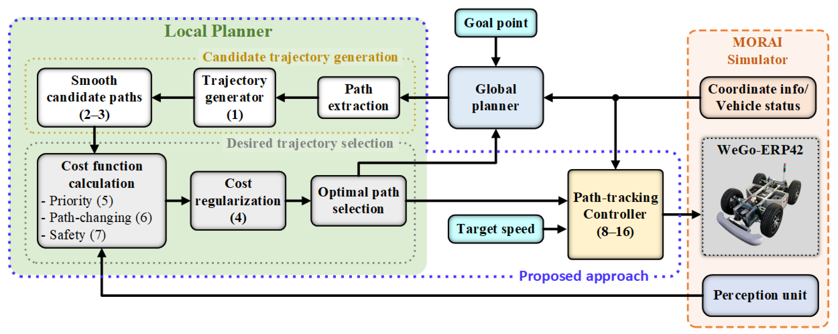
2. Proposed Approach

This section provides the operational details of our proposed approach. Figure 1 illustrates the overall structure of the system and how this solution operates. The motion planner consists of two parts: a global planner and a local planner. The primary focus of this study was an improved local planning strategy. Specifically, it is divided into two main periods: candidate path generation and expected path selection. The generated candidate trajectory is smoothed before evaluation to decide the best path output. Then, it is supplied as input to the path-tracking module. If a safe and smooth obstacle-free trajectory is selected, the future pose state of the AV is then estimated utilizing the LPV model error. Finally, to obtain the ideal control sequence, a quadratic programming scheme is deployed to solve for the cost function. The MPC controller is then instructed to operate the vehicle using the first component of the control sequence, which is the desired acceleration and speed.

2.1. Local Planning

2.1.1. Candidate Trajectory Generation

The local trajectory planner algorithm creates roll-outs through a three-step process. Firstly, a specific section of the global path is extracted, based on the current AV position and maximum planning distance. A series of path points, ${\mathbf{p}}_j(x_j,y_j),\forall j\in [0,n]$ corresponds to each candidate’s path with its direction ${\theta }_j=\frac{y_{j+1}-y_j}{x_{j+1}-x_j}$. After sampling, there is a total number of candidate paths of $(s+1)$, among which the nominal path is the $(s/2)$th path.

Next, the newly sampled perpendicular points are calculated from the global path. For the jth path point ${\mathbf{p}}_{ij}(x_{ij},y_{ij}),\forall i\in [0,s]$ of the ith candidate path, we obtain

$$\begin{array}{cc}\hfill & x_{ij}=x_i-dcos({tan}^{-1}\left({\theta }_j\right)+\pi /2),\hfill \\ \hfill & y_{ij}=y_j-dsin({tan}^{-1}\left({\theta }_j\right)+\pi /2).\hfill \end{array}$$

(1)

where

$$d=\left\{\begin{array}{cc}{d}_l=cos\left({tan}^{-1}\left({\theta }_{ij}\right)\right)(y_{ij}-y_i)-sin\left({tan}^{-1}\left({\theta }_{ij}\right)\right)(x_{ij}-x_i),\hfill & \mathrm{for}j=0,1,\cdots ,l,\hfill \\ d_m=d_l+\frac{d_n-d_l}{n-l}(j-l),\hfill & \mathrm{for}j=l+1,l+2,\cdots ,m,\hfill \\ d_n=h\left(i-\frac{s}{2}\right),\hfill & \mathrm{for}j=m+1,m+2,\cdots ,n,\hfill \end{array}\right.$$

${\theta }_{ij}$ denotes the direction of the waypoint ${\mathbf{p}}_{ij}(x_{ij},y_{ij})$ on the candidate path, and h is the horizontal spacing of the candidate paths. The algorithm used to generate roll-out trajectories is shown in Algorithm A1.

It is noteworthy that the generated candidate paths (1) are not smooth at the junction of the three stages, which significantly affects later tracking control tasks. Thus, it is necessary to smooth each candidate to improve curvature before providing the path-tracking module, which is conducive to smoother steering. To this end, a nonlinear iterative optimization technique, namely the gradient descent method, is deployed to reject the disruption of roll-outs resulting from the sampling process, as seen in Algorithm A2. The smoothness optimization objective function S is defined as follows:

$$\mathcal{F}=\underset{{\mathcal{F}}_d:\mathrm{deviation}\mathrm{evaluation}}{\underbrace{\sum _{i=0}^m\left\{{\left(x_i+x_i^r\right)}^2+{\left(y_i+y_i^r\right)}^2\right\}}}+\underset{{\mathcal{F}}_s:\mathrm{smoothness}\mathrm{evaluation}}{\underbrace{\sum _{i=0}^{m-1}\left\{{\left(x_{i-1}+x_{i+1}-2x_i\right)}^2+{\left(y_{i-1}+y_{i+1}-2y_i\right)}^2\right\}}}$$

(2)

where ${\mathbf{p}}_i^r\left(x_i^r,y_i^r\right)$ is the original path point corresponding to the optimized discrete path point, ${\mathbf{p}}_i(x_i,y_i)$. The gradient of $\mathcal{F}$ is obtained by taking its partial derivative with respect to $x_i$ and $y_i$, respectively, in the following:

$$\begin{array}{cc}\hfill \frac{\partial {\mathcal{F}}_d}{\partial x_i}& =2\left(x_i-2x_i^r\right),\hfill \\ \hfill \frac{\partial {\mathcal{F}}_d}{\partial y_i}& =2\left(y_i-2y_i^r\right),\hfill \\ \hfill \frac{\partial {\mathcal{F}}_s}{\partial x_i}& =2\left(x_{i-2}-4x_{i-1}+6x_i-4x_{i+1}+x_{i+2}\right),\hfill \\ \hfill \frac{\partial {\mathcal{F}}_s}{\partial y_i}& =2\left(y_{i-2}-4y_{i-1}+6y_i-4y_{i+1}+y_{i+2}\right).\hfill \end{array}$$

(3)

After the path points are optimized, a smooth candidate path is obtained, which is an input into the desired path selector for evaluation, and the desired path is selected.

2.1.2. Desired Trajectory Selection

The optimal path selector is implemented to evaluate each trajectory, which minimizes a linear combination of multiple cost functions among candidate paths to choose the best possible trajectory. The total cost values are expressed as follows:

$$\begin{array}{c}\hfill J_{total}={\omega }_z\sum _{z=0}^3\frac{J_{iz}}{{\sum }_{i=0}^n{J}_{iz}}\end{array}$$

(4)

where $J_{iz}$, $z=\left\{1,2,3\right\}$ represent the priority cost, path-change cost, and safety cost, respectively, and ${\omega }_z$ are the cost weight coefficients corresponding to the above costs.

The priority cost is a measure of the attractiveness of the central path to the vehicle. The central path, namely the nominal path, has the highest priority, and the priority cost can be written as

$$\begin{array}{c}\hfill J_{i1}=\left|h\left(i-\frac{s}{2}\right)\right|\end{array}.$$

(5)

The path-changing cost refers to the cost required for the vehicle to switch from the current path to each candidate path. The absolute value of the relative distance between the current path, $i_c$ and each candidate path, i is used to measure the path-changing cost. This cost term is represented as follows:

$$\begin{array}{c}\hfill J_{i2}=\left|h\left(i-i_c\right)\right|.\end{array}$$

(6)

For the safety cost, we evaluate all the probabilities of a vehicle colliding with an obstacle nearby. The size of the collision cost is represented by the sum of the absolute values of the relative distances between the current path and the outline points of all obstacles. In addition, although the obstacle detection function is not the primary focus of this study, its depiction presents several trade-offs between accuracy and performance.

For any outline point ${\mathbf{p}}_i(x_i,y_i)$ in the obstacle point set, let the closest path point on the candidate path be ${\mathbf{p}}_{iv}(x_{iv},y_{iv})$, $\forall v\in [0,N]$ with N being the number of obstacle contour points. According to (1), the offset distance $d_{iv}$ is the gap between the obstacle point and the candidate path. For the ith candidate path, its safe cost $J_{i3}$ is

$$\begin{array}{c}\hfill J_{i3}=\sum _{v=0}^{N-1}\left|d_{iv}\right|\end{array}$$

(7)

where $d_{iv}=cos(ta{n}^{-1}\left({\theta }_{iv}\right)(y_{iv}-y_i)-sin(ta{n}^{-1}\left({\theta }_{iv}\right)(x_{iv}-x_i)$.

According to (4)–(7), it is possible to determine the cost of each valid candidate path and then choose the one with the lowest cost as the final local path to be executed, thereby completing the local obstacle avoidance path planning in one cycle.

2.2. Path-Tracking Approach

In order to represent the nominal LPV dynamics, Jacobian matrices are computed along the nominal trajectory, which include the nonlinear dynamics as scheduling parameters [37]. The LPV model is capable of capturing nonlinear dynamics within a bounded region over the prediction horizon. Thus, the tracking error of the LPV–MPC is constrained within a small bound. By using the Euler method [32], the discrete-time version of the nonlinear system can be described as follows:

$$\begin{array}{c}\hfill x(k+1)=x\left(k\right)+\Delta tf\left(x\right(k),u(k\left)\right)\end{array}$$

(8)

where $x={[v_x,v_y,\omega ,\dot{\omega },x_d,y_d]}^{\top }\in {\mathbb{R}}^p$ denotes the six-dimensional state vector; $u\left(t\right)={[\delta ,a]}^{\top }\in {\mathbb{R}}^q$ denotes the control input; $\Delta t$ and k denotes the step size and step index, respectively. According to the Taylor series, (8) is expanded around the referenced point $(x_r,u_r)$ at ${\dot{x}}_r=f(x_r,u_r)$, and we obtain:

$$\begin{array}{c}\hfill x(k+1)\approx x\left(k\right)+\Delta t\left[f(x_r,u_r)+f_{x,r}(x-x_r)+f_{u,r}(u-u_r)\right]\end{array}$$

(9)

where $f_{x,r}$ and $f_{u,r}$ denote the Jacobians of x and u, respectively, assessed around the referenced points $(x_r,u_r)$. Then, (9) can be rewritten as follows:

$$\begin{array}{cc}\hfill x_e(k+1)& =A\left(k\right)x_e\left(k\right)+B\left(k\right)u_e\left(k\right),\hfill \\ \hfill y_e\left(k\right)& =C\left(k\right)x_e\left(k\right)\hfill \end{array}$$

(10)

where $x_e\left(k\right)=x\left(k\right)-x_r\left(k\right)$ and $u_e\left(k\right)=u\left(k\right)-u_r\left(k\right)$ denote the tracking error and control input at each time instant; the system matrices $A\in {\mathbb{R}}^{p\times p}$, $B\in {\mathbb{R}}^{p\times q}$ and $C\in {\mathbb{R}}^{n\times p}$ are derived in Appendix B.

The fundamental idea of the LPV–MPC generates control command sequences to track the nominal system states, which can be optimized to reduce tracking errors over a finite horizon by previewing the scheduling parameter sequences. From (10), the predicted outputs, $y_e(k+i|k)$, and the control inputs, $u_e(k+i|k)$, we have

$$\begin{array}{c}\hfill \left[\begin{array}{c}{y}_e(k+1|k)\\ y_e(k+2|k)\\ ⋮\\ y_e(k+N_y|k)\end{array}\right]=\left[\begin{array}{c}CA\\ C{A}^2\\ ⋮\\ C{A}^{N_y}\end{array}\right]x\left(k\right|k)+\left[\begin{array}{c}CB\\ CAB+CB\\ ⋮\\ \sum _{i=1}^{N_y}C{A}^{i-1}B\end{array}\right]u_e(k-1)+\mathsf{\Psi }\left[\begin{array}{c}{u}_e\left(k\right)\\ u_e(k+1)\\ ⋮\\ u_e(k+N_c-1)\end{array}\right]\end{array}$$

(11)

where $\mathsf{\Psi }=\left[\begin{array}{cccc}CB& 0& \cdots & 0\\ CAB+CB& CB& 0& 0\\ ⋮& ⋮& \ddots & ⋮\\ {\sum }_{i=1}^{N_y}C{A}^{i-1}B& {\sum }_{i=1}^{N_y-1}C{A}^{i-1}B& \cdots & {\sum }_{i=1}^{N_y-N_c+1}C{A}^{i-1}B\end{array}\right]$.

At time instance k, the optimal input sequences of the control horizon are calculated by solving the optimization problem as follows:

$$\begin{array}{cc}\hfill \underset{U_e}{\min }& J(U_e,x_e\left(k\right))=\sum _{i=0}^{N_y-1}\left({∥Q{y}_e(k+1|k)∥}^2+{∥R{u}_e(k+i|k)∥}^2\right)\hfill \\ \hfill \mathrm{subj}.\mathrm{to}& x_e(k+i+1|k)=A(k+i|k)x_e(k+i|k)+B(k+1|k)u_e(k+i|k)\hfill \\ \hfill & y_e(k+i|k)=C(k+i|k)x_e(k+i|k)\hfill \\ \hfill & x_e\left(k\right|k)=x_e\left(k\right)=x_0-x_0^{*},x_e\left(k\right)\in \delta \mathbf{X},\hfill \\ \hfill & y_e\left(k\right|k)=y_e\left(k\right)=y_0-x_0^{*},y_e\left(k\right)\in \delta \mathbf{Y},\hfill \\ \hfill & U_e=\mathrm{col}\left\{u_e\left(k\right|k),\cdots ,u_e(N_y-1_k|k)\right\},u_e\left(i\right|k)\in \mathbf{U}\hfill \end{array}$$

(12)

where the cost function $J(U_e,x_e\left(k\right))$ is chosen as a quadratic form; $\delta \mathbf{U}\in \mathbf{U}$ and $\delta \mathbf{X}\in \mathbf{X}$ denote the constraints of control inputs and states, respectively; $N_c$ and $N_y$ denote the inputs and outputs of the predictive horizon, respectively; $U_e$ is the predicted input sequences; $y_e(k+i|k)$ is the current predicted output at time k, $u_e(k+i|k)$ is the predicted input vector, which can be defined as follows:

$$\begin{array}{c}\hfill u_e\left(k_i\right|k)=u(k+i|k)-u(k+i-i|k)\end{array}$$

(13)

$Q=Q^{\prime }\ge 0,R=R^{\prime }>0$ are the weighting matrices of the predicted outputs and control inputs, respectively.

The optimal control input vector is defined as

$$\begin{array}{c}\hfill U_e^{*}:=U_e^{*}\left(k\right),\cdots ,U_e^{*}(k+Nu-1)\end{array}$$

(14)

and the new inputs as

$$\begin{array}{c}\hfill u(k+i|k)=u(k+i-1|k)+u_e(k+i|k)\end{array}$$

(15)

Then, the first element of the control inputs, $u_e^{*}\left(k\right)$, is taken as the current optimal input and the resulting control law is derived as the following:

$$\begin{array}{c}\hfill u^{*}\left(k\right)=u(k-1)+u_e^{*}\left(k\right).\end{array}$$

(16)

The system shifts the control variable to the next step and re-predicts the output of the next step by solving the optimization problem (12) over a shifted horizon. It is based on the state information at a new step and based on an updated linear model computed by linearizing (10) and previous input. This cycle is repeated until the entire control process is completed.

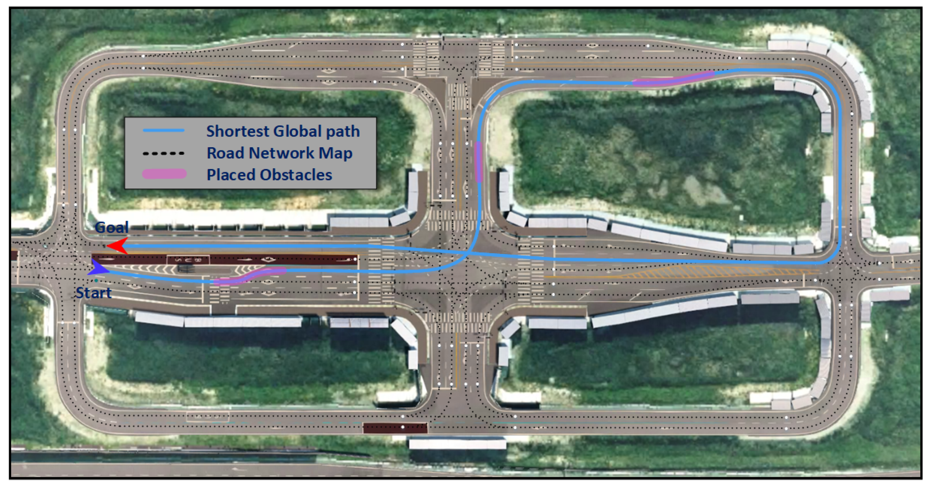
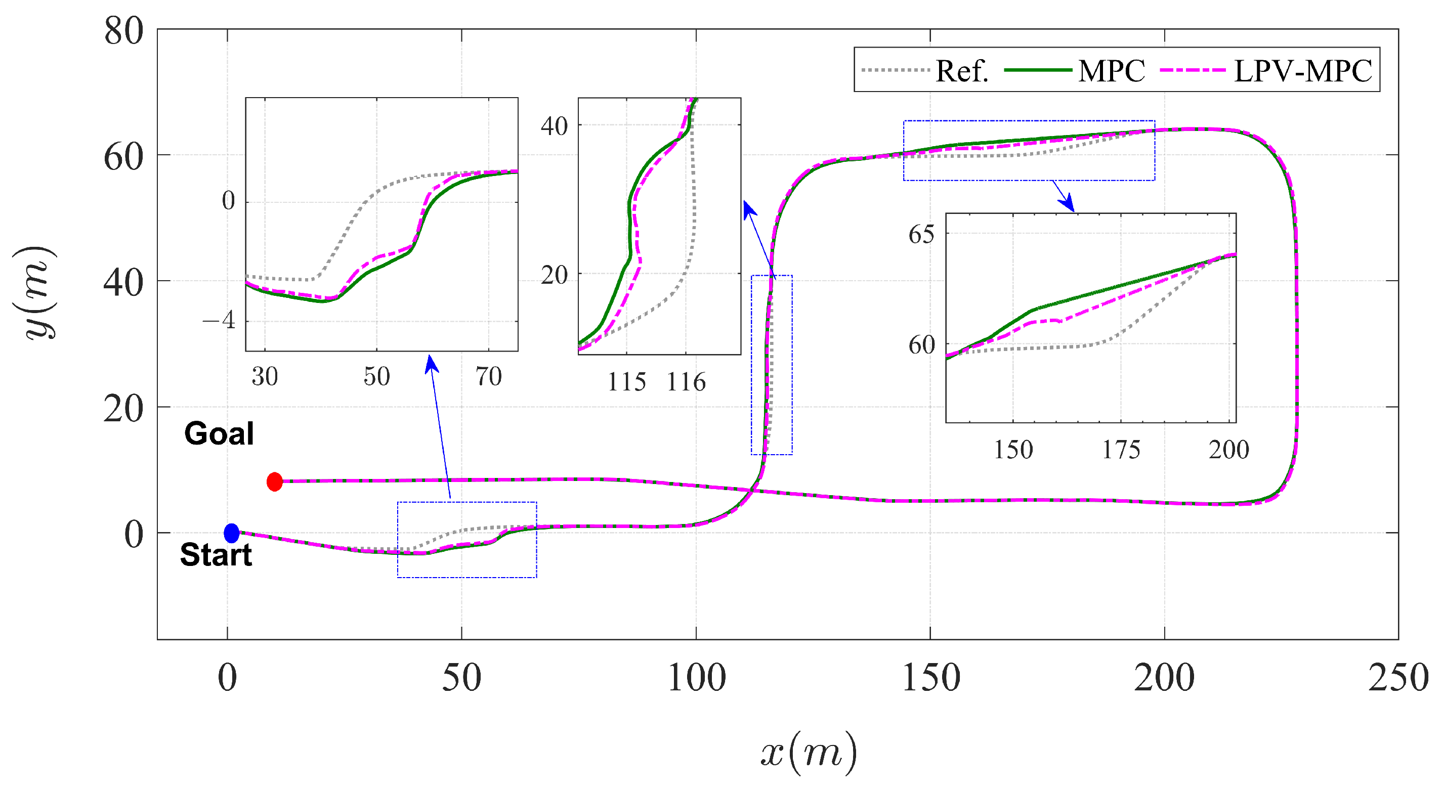
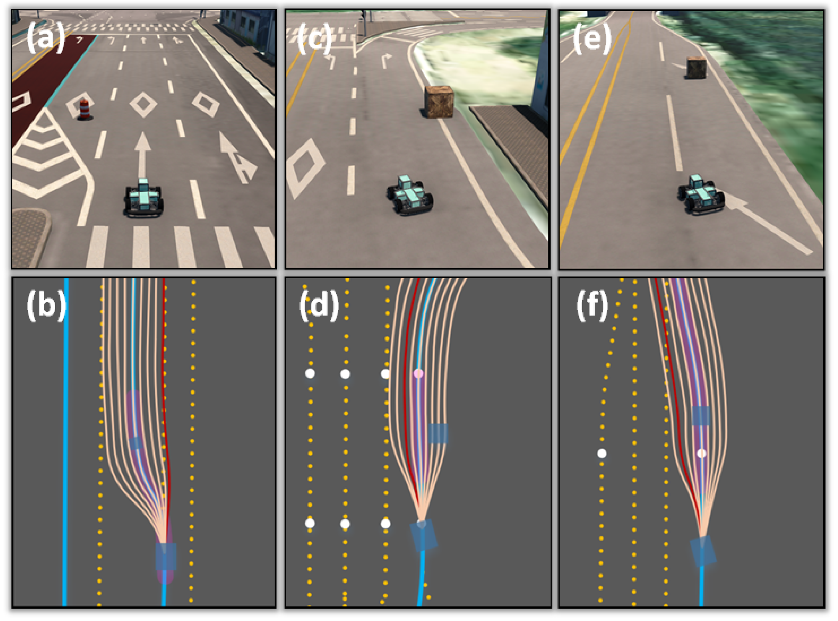
3. Simulation Validation

3.1. Environment Setup

The motion planning and path-tracking control strategies are evaluated by first finding a global trajectory for the whole autonomous driving system and then executing the local planner. To do so, a start and a target position (marked by blue and red arrows, respectively) are set as input and then the road network map is extracted to find the shortest path routing by the global planner, based on Dijkstra’s algorithm. The whole information of the expected path can be provided to the local planner while complying with traffic regulations. To establish testing scenarios, we comprehensively design a series of trials on the MORAI simulator [35], and several obstacles are placed on the road to analyze and evaluate the capability of the proposed control strategy in the local planner. Meantime, the obstacle status is obtained by utilizing the published data from the simulator. For the control design, the optimal control problem is solved every sampling period of 30 Hz to find the appropriate control actions. The prediction horizon and control horizon are chosen as $N_y=20$ and $N_c=10$. The expected speed of the vehicle is set to 8 m/s. To guarantee stability and smoothness, the limits $\mathbf{U}=\pm {\left[\begin{array}{cc}\frac{\pi }{4}& 1.25\end{array}\right]}^{\top }$ and $\mathbf{X}=\pm {\left[\begin{array}{cccccc}8& 2& 3& 3& 1& 10\end{array}\right]}^{\top }$ bound the front steering angle and longitudinal acceleration of the vehicle. The elements of the diagonal weighting matrices Q and R are set to $1.25$ and $0.1$, respectively. Groups of comparative simulations were carried out with the following conditions: (1) In order to sufficiently illustrate the effectiveness of the proposed method, trials using MPC and LPV–MPC, respectively, were considered; (2) Simultaneously, a demonstration using a global path as a reference with multiple placed obstacles was used to evaluate the control accuracy and robustness.

3.2. Results

The global trajectory is found as the shortest path routing, while fulfilling traffic law constraints, as illustrated in Figure 2, in which the vehicle starts to move at the coordinate (0, 0). To evaluate the proposed control approach, the obstacles were placed at different locations on the route with their coordinates being 1st obstacle $(45,0)$, 2nd obstacle $(116,25)$, 3rd obstacle $(170,60)$. The results of the comprehensive trial are depicted in Figure 3. The gray dotted line is the reference path as the shortest global path, and the green line and the purple dotted line are the output trajectories controlled by the proposed motion planning combined with the MPC and LPV–MPC technique, respectively. Generally, it can be seen that both approaches could basically overlap with the reference trajectory, but the difference was more obvious at the locations where obstacles appeared, as shown in partial enlargement.

The series of obstacles are illustrated in Figure 4 with partial enlargement of the visualization, respectively. The order of candidate paths is marked from right to left of the car starting from 1st to 9th, where the light orange lines are the candidate paths, and the red line is the selected optimal path. Correspondingly, the total cost and its respective cost values of the optimal path during the comprehensive simulation are depicted in Figure 5. In this figure, the dotted pink line is the priority cost with a constant coefficient value for each individual path. The dotted green line is the path-changing cost and its change indicates the number of lane-changing times of the vehicle. The dotted orange line is the collision cost, which represents the safety of the candidate path, i.e., the main influencing factor in motion planning. In detail, at t = 7–12 s the vehicle position was $(30,0)$, the distance to the 1st obstacles was 15 m, the vehicle switched frame 5th path to 1st path to pass on the right side of the $ob{s}^{1\mathrm{st}}$ obstacle (Figure 4a,b) with the total cost of the optimal path being between 0.35–0.5. In the meantime, the peaks of the collision cost and the path-changing costs were up to $0.9$ and $0.5$, respectively. Next, when the position of the vehicle was $(114.5,12)$ at t = 22–25 s, the optimal path switched from 5th path to 7th path. The path-changing cost and the collision cost were in the same direction as the peak values $0.65$ and $0.4$, respectively. This meant that the vehicle passed on the left side of the 2nd obstacle (Figure 4c,d) with a total cost of $0.65$. At $t=$ 28–34 s, the vehicle was at $(160,60)$, passing through 3rd obstacle along 8th path (Figure 4e,f). Since this obstacle appeared near the merge lane, the local planner adjusted to the left lane earlier than the expected path, with the total cost varying from $0.02$ to $0.55$. Although there were some obstacles that appeared to obstruct the target road, the above results indicate that the suggested approach is capable of evaluating and handling risky situations safely and quickly.

In order to further demonstrate the efficacy of the suggested approach, Figure 6 indicates the cross-tracking error (CTE) of the MPC and LPV–MPC methods, respectively, versus the optimal path (Figure 6a) and the velocity versus time (Figure 6b). The CTE is defined here as the distance from the vehicle coordinate position versus the optimal path, i.e., $y_e=v_{x}sin{\theta }_e+v_{y}cos{\theta }_e$. The results in Figure 6a show that the CTE values had three oscillations corresponding to three locations of obstacles, since the obstacles were avoided considering the safety distance of the vehicle. Meanwhile, all candidate paths gradually approached the reference trajectory from the position of the vehicle, which indicates that the proposed motion planning approach considered the current positional state of the vehicle. However, there were significant differences when integrating each path-tracking approach. The peak error of the LPV–MPC approach was within 0.25 m at t = 8–14 s, while the peak error of the MPC approach was slightly larger at 0.38 m at the same time. At t = 23 s, it was absolutely clear that the peak error of MPC was 0.7 m, and the corresponding maximum error of LPV–MPC was still 0.28 m at this time. Similarly, the peak CTE of the LPV–MPC approach was smaller than that of MPC at t = 32 s, and, in turn, 0.2 m versus 0.5 m. During the remaining phase, the CTE was quite small, which meant that it nearly coincided with the optimal path. On the other hand, as illustrated in Figure 6b, the velocity-tracking performance of the proposed motion planning when combined with the LPV–MPC approach was also better than that of MPC. It can be seen that, in the case of a dynamic environment with obstacle avoidance, the LPV–MPC strategy could be suitably evaluated under different conditions with high precision.

As shown in Figure 7, the control inputs of the front steering angle and the longitudinal acceleration are displayed as time evolved, respectively. Although the LPV–MPC integrated into the proposed motion planning approach with significantly smaller control effort, the control performance was better than the MPC approach. Generally, the tracking performances illustrated that both the LPV–MPC and MPC could effectively maintain the position constraint in a reasonable range. In particular, compared with the MPC approach, the LPV–MPC approach could not only improve the lateral tracking accuracy of the vehicle but also speed up the longitudinal error convergence under initial conditions. As a result, the proposed LPV–MPC method exhibited high accuracy and robustness in trajectory tracking. Therefore, the AV using the LPV–MPC method could track the desired trajectory completely. Figure 8 expresses the elapsed time when computing with a mean time of 0.6985 s and 0.0347 s for a prediction horizon of 20 steps of the MPC strategy and LPV–MPC approach, respectively. It implies that computational time improvement was achieved when using the LPV–MPC strategy. The several peaks could be due to the appearance of obstacles, causing the optimizer to deal with somewhat complicated and, hence, more time-consuming situations.

4. Conclusions

In this paper, an integrated motion planning and control framework was proposed for the AV. The path planner incorporates the path-following strategy to deliver a good balance of fast decisions, safety, and accuracy by running both modules in parallel. The proposed motion planning module, composed of a behavior selector, is developed for obstacle avoidance, while generating parametric online reference paths. It satisfies the constraints on the allowable curvature of a given AV, as well as different initial states. Depending on the scene, the motion planner generates trajectories through intermediate safe spots to avoid obstacles. Meanwhile, the LPV–MPC is simultaneously adopted in the path-tracking module to improve path-tracking accuracy and compared with the MPC control. The proposed method was evaluated in the MORAI simulator, in a scenario with several bends and various obstacles. The simulation results demonstrated that the motion planner is capable of handling these feasibility checks and risk evaluation situations safely and quickly. Meantime, the robustness and accuracy of the path-tracking task are guaranteed by the LPV–MPC approach with rather small peaks of the CTE within 0.28 m. It can generate an appropriate velocity that varies smoothly, which is helpful to the vehicle’s stability of control. All of these indicate that it is a promising control scheme for practical applications.

In future work, the proposed algorithm will be analyzed further and generalized in a complex environment in the presence of other vehicles. The predictive ability in regard to the tendency of obstacles to move will be developed to improve safety as well as offer higher precision. Then, it will be applied in real-time platforms for a comprehensive assessment of performance.

References

1. Bin-Nun, A.Y.; Derler, P.; Mehdipour, N.; Tebbens, R.D. How should autonomous vehicles drive? Policy, methodological, and social considerations for designing a drive. Humanit. Soc. Sci. Commun. 2022, 9, 299. [Google Scholar] [CrossRef]
2. Parekh, D.; Poddar, N.; Rajpurkar, A.; Chahal, M.; Kumar, N.; Joshi, G.P.; Cho, W. A Review on Autonomous Vehicles: Progress, Methods and Challenges. Electronics 2022, 11, 2162. [Google Scholar] [CrossRef]
3. Huang, Y.; Wang, H.; Khajepour, A.; Ding, H.; Yuan, K.; Qin, Y. A Novel Local Motion Planning Framework for Autonomous Vehicles Based on Resistance Network and Model Predictive Control. IEEE Trans. Veh. Technol. 2020, 69, 55–66. [Google Scholar] [CrossRef]
4. Wang, H.; Huang, Y.; Khajepour, A.; Zhang, Y.; Rasekhipour, Y.; Cao, D. Crash Mitigation in Motion Planning for Autonomous Vehicles. IEEE Trans. Intell. Transp. Syst. 2019, 20, 3313–3323. [Google Scholar] [CrossRef]
5. Daoud, M.A.; Mehrez, M.W.; Rayside, D.; Melek, W.W. Simultaneous Feasible Local Planning and Path-Following Control for Autonomous Driving. IEEE Trans. Intell. Transp. Syst. 2022, 23, 16358–16370. [Google Scholar] [CrossRef]
6. Wang, Q.; Li, J.; Yang, L.; Yang, Z.; Li, P.; Xia, G. Distributed Multi-Mobile Robot Path Planning and Obstacle Avoidance Based on ACO–DWA in Unknown Complex Terrain. Electronics 2022, 11, 2144. [Google Scholar] [CrossRef]
7. Liang, Y.; Li, Y.; Khajepour, A.; Huang, Y.; Qin, Y.; Zheng, L. A Novel Combined Decision and Control Scheme for Autonomous Vehicle in Structured Road Based on Adaptive Model Predictive Control. IEEE Trans. Intell. Transp. Syst. 2022, 23, 16083–16097. [Google Scholar] [CrossRef]
8. Chen, C.; Rickert, M.; Knoll, A. Kinodynamic motion planning with Space-Time Exploration Guided Heuristic Search for car-like robots in dynamic environments. In Proceedings of the 2015 IEEE/RSJ International Conference on Intelligent Robots and Systems (IROS), Hamburg, Germany, 28 September–2 October 2015; pp. 2666–2671. [Google Scholar]
9. Ajanovic, Z.; Lacevic, B.; Shyrokau, B.; Stolz, M.; Horn, M. Search-Based Optimal Motion Planning for Automated Driving. In Proceedings of the 2018 IEEE/RSJ International Conference on Intelligent Robots and Systems (IROS), Madrid, Spain, 1–5 October 2018; pp. 4523–4530. [Google Scholar]
10. Jeon, J.h.; Karaman, S.; Frazzoli, E. Anytime computation of time-optimal off-road vehicle maneuvers using the RRT*. In Proceedings of the 2011 50th IEEE Conference on Decision and Control and European Control Conference, Orlando, FL, USA, 12–15 December 2011; pp. 3276–3282. [Google Scholar]
11. Montes, N.; Mora, M.C.; Tornero, J. Trajectory Generation based on Rational Bezier Curves as Clothoids. In Proceedings of the 2007 IEEE Intelligent Vehicles Symposium, Istanbul, Turkey, 13–15 June 2007; pp. 505–510. [Google Scholar]
12. Berglund, T.; Brodnik, A.; Jonsson, H.; Staffanson, M.; Soderkvist, I. Planning Smooth and Obstacle-Avoiding B-Spline Paths for Autonomous Mining Vehicles. IEEE Trans. Autom. Sci. Eng. 2010, 7, 167–172. [Google Scholar] [CrossRef] [Green Version]
13. Glaser, S.; Vanholme, B.; Mammar, S.; Gruyer, D.; Nouvelière, L. Maneuver-Based Trajectory Planning for Highly Autonomous Vehicles on Real Road With Traffic and Driver Interaction. IEEE Trans. Intell. Transp. Syst. 2010, 11, 589–606. [Google Scholar] [CrossRef]
14. Moreau, J.; Melchior, P.; Victor, S.; Aioun, F.; Guillemard, F. Path planning with fractional potential fields for autonomous vehicles. IFAC-PapersOnLine 2017, 50, 14533–14538. [Google Scholar] [CrossRef]
15. Lim, W.; Lee, S.; Sunwoo, M.; Jo, K. Hierarchical Trajectory Planning of an Autonomous Car Based on the Integration of a Sampling and an Optimization Method. IEEE Trans. Intell. Transp. Syst. 2018, 19, 613–626. [Google Scholar] [CrossRef]
16. Jeong, D.; Ko, G.; Choi, S.B. Estimation of sideslip angle and cornering stiffness of an articulated vehicle using a constrained lateral dynamics model. Mechatronics 2022, 85, 102810. [Google Scholar] [CrossRef]
17. Barbosa, F.M.; Marcos, L.B.; da Silva, M.M.; Terra, M.H.; Junior, V.G. Robust path-following control for articulated heavy-duty vehicles. Control Eng. Pract. 2019, 85, 246–256. [Google Scholar] [CrossRef] [Green Version]
18. Zhao, W.; Ma, X.; Nie, Z. DDPG-based controller of enhanced adaptive cruise control with lane-change assistance for an articulated vehicle. Proc. Inst. Mech. Eng. Part J. Automob. Eng. 2022. [Google Scholar] [CrossRef]
19. Polack, P. Consistency and Stability of Hierarchical Planning and Control Systems for Autonomous Driving. Ph.D. Dissertation, PSL Research University, Paris, France, October 2018. [Google Scholar]
20. Koenig, S.; Likhachev, M. D*lite. In Proceedings of the Eighteenth National Conference on Artificial Intelligence, Edmonton, AB, Canada, 28 July–1 August 2002; American Association for Artificial Intelligence: Washington, DC, USA, 2002; pp. 476–483. [Google Scholar]
21. Simmons, R. The curvature-velocity method for local obstacle avoidance. In Proceedings of the IEEE International Conference on Robotics and Automation, Minneapolis, MN, USA, 22–28 April 1996; Volume 4, pp. 3375–3382. [Google Scholar]
22. Li, X.; Sun, Z.; Kurt, A.; Zhu, Q. A sampling-based local trajectory planner for autonomous driving along a reference path. In Proceedings of the 2014 IEEE Intelligent Vehicles Symposium Proceedings, Dearborn, MI, USA, 8–11 June 2014; pp. 376–381. [Google Scholar]
23. Thrun, S.; Montemerlo, M.; Dahlkamp, H.; Stavens, D.; Aron, A.; Diebel, J.; Fong, P.; Gale, J.; Halpenny, M.; Hoffmann, G.; et al. Stanley: The robot that won the DARPA Grand Challenge. J. Field Robot. 2006, 23, 661–692. [Google Scholar] [CrossRef]
24. Xu, T.; Wang, D.; Zhang, W. A non-overshooting controller for vehicle path following. Trans. Inst. Meas. Control. 2021, 43, 2282–2291. [Google Scholar] [CrossRef]
25. Morales, Y.; Watanabe, A.; Ferreri, F.; Even, J.; Ikeda, T.; Shinozawa, K.; Miyashita, T.; Hagita, N. Including human factors for planning comfortable paths. In Proceedings of the 2015 IEEE International Conference on Robotics and Automation (ICRA), Seattle, WA, USA, 26–30 May 2015; pp. 6153–6159. [Google Scholar]
26. Shojaei, S.; Hanzaki, A.R.; Azadi, S.; Saeedi, M.A. A novel decision-making unit for automated maneuver of articulated vehicles in real traffic situations. Proc. Inst. Mech. Eng. Part J. Automob. Eng. 2020, 234, 152–171. [Google Scholar] [CrossRef]
27. Fehér, Á.; Aradi, S.; Bécsi, T. Online Trajectory Planning with Reinforcement Learning for Pedestrian Avoidance. Electronics 2022, 11, 2346. [Google Scholar] [CrossRef]
28. Wiberg, V.; Wallin, E.; Nordfjell, T.; Servin, M. Control of Rough Terrain Vehicles Using Deep Reinforcement Learning. IEEE Robot. Autom. Lett. 2022, 7, 390–397. [Google Scholar] [CrossRef]
29. Song, R.; Ye, Z.; Wang, L.; He, T.; Zhang, L. Autonomous Wheel Loader Trajectory Tracking Control Using LPV-MPC. In Proceedings of the 2022 American Control Conference (ACC), Atlanta, GA, USA, 8–10 June 2022; pp. 2063–2069. [Google Scholar]
30. Fu, T.; Zhou, H.; Liu, Z. NMPC-Based Path Tracking Control Strategy for Autonomous Vehicles with Stable Limit Handling. IEEE Trans. Veh. Technol. 2022, 71, 12499–12510. [Google Scholar] [CrossRef]
31. Zhai, L.; Wang, C.; Hou, Y.; Liu, C. MPC-Based Integrated Control of Trajectory Tracking and Handling Stability for Intelligent Driving Vehicle Driven by Four Hub Motor. IEEE Trans. Veh. Technol. 2022, 71, 2668–2680. [Google Scholar] [CrossRef]
32. Vo, C.P.; Lee, J.; Jeon, J.H. Robust Adaptive Path Tracking Control Scheme for Safe Autonomous Driving via Predicted Interval Algorithm. IEEE Access 2022, 10, 124333–124344. [Google Scholar] [CrossRef]
33. Tian, Y.; Yao, Q.; Hang, P.; Wang, S. A Gain-Scheduled Robust Controller for Autonomous Vehicles Path Tracking Based on LPV System With MPC and H. IEEE Trans. Veh. Technol. 2022, 71, 9350–9362. [Google Scholar] [CrossRef]
34. Peng, H.; Wang, W.; An, Q.; Xiang, C.; Li, L. Path Tracking and Direct Yaw Moment Coordinated Control Based on Robust MPC With the Finite Time Horizon for Autonomous Independent-Drive Vehicles. IEEE Trans. Veh. Technol. 2020, 69, 6053–6066. [Google Scholar] [CrossRef]
35. MORAI. Available online: https://www.morai.ai/product (accessed on 1 February 2022).
36. Chu, D.; Li, H.; Zhao, C.; Zhou, T. Trajectory Tracking of Autonomous Vehicle Based on Model Predictive Control With PID Feedback. IEEE Trans. Intell. Transp. Syst. 2023, 24, 2239–2250. [Google Scholar] [CrossRef]
37. Rotondo, D.; Puig, V.; Nejjari, F.; Witczak, M. Automated generation and comparison of Takagi–Sugeno and polytopic quasi-LPV models. Fuzzy Sets Syst. 2015, 277, 44–64. [Google Scholar] [CrossRef] [Green Version]
Figure 1. Overall architecture of our AV self-driving scheme with corresponding equation numbers.
Electronics 12 01566 g001
Figure 2. The optimal shortest path of global planning with the internal map structure consisting of center lines and nodes of the road network connections.
Electronics 12 01566 g002
Figure 3. Results of a comprehensive simulation using the proposed motion planning and path tracking framework.
Electronics 12 01566 g003
Figure 4. The response of the proposed approach at different positions of the obstacles; The simulation scene (above) and the candidate and optimal paths (below) correspond to the 1st obstacle (a,b), the 2nd obstacle (c,d) and the 3rd obstacle (e,f), respectively.
Electronics 12 01566 g004
Figure 5. The costs of the optimal path.
Electronics 12 01566 g005
Figure 6. Response performances with respect to integrating MPC and LPV–MPC methods, respectively; (a) The cross-tracking errors versus the optimal path; (b) The longitudinal velocities versus the target velocity.
Electronics 12 01566 g006
Figure 7. The standard deviations of the optimal control signals when using MPC and LPV-MPC path tracking methods, respectively, (a) The front steering angle; (b) The longitudinal acceleration.
Electronics 12 01566 g007
Figure 8. Computational effort comparison; (a,b) Elapsed time per iteration of the MPC strategy and LPV–MPC approach, respectively.
Electronics 12 01566 g008
Disclaimer/Publisher’s Note: The statements, opinions and data contained in all publications are solely those of the individual author(s) and contributor(s) and not of MDPI and/or the editor(s). MDPI and/or the editor(s) disclaim responsibility for any injury to people or property resulting from any ideas, methods, instructions or products referred to in the content.