A Hybrid Improved-Whale-Optimization–Simulated-Annealing Algorithm for Trajectory Planning of Quadruped Robots

Abstract

Traditional trajectory-planning methods are unable to achieve time optimization, resulting in slow response times to unexpected situations. To address this issue and improve the smoothness of joint trajectories and the movement time of quadruped robots, we propose a trajectory-planning method based on time optimization. This approach improves the whale optimization algorithm with simulated annealing (IWOA-SA) together with adaptive weights to prevent the whale optimization algorithm (WOA) from falling into local optima and to balance its exploration and exploitation abilities. We also use Markov chains of stochastic process theory to analyze the global convergence of the proposed algorithm. The results show that our optimization algorithm has stronger optimization ability and stability when compared to six representative algorithms using six different test function suites in multiple dimensions. Additionally, the proposed optimization algorithm consistently constrains the angular velocity of each joint within the range of kinematic constraints and reduces joint running time by approximately 6.25%, which indicates the effectiveness of this algorithm.

1. Introduction

Compared with wheeled robots, legged robots are more suitable for tough terrain and complex environments [1]. The quadruped robots can freely select contact points while making contact with the environment [2]. Therefore, they can be used in the wild rescue field, to carry payloads in construction sites, and to climb stairs [3]. Moreover, the operating environment of the legged robot is mostly uneven, and the quadruped robot can adapt to most of the non-flat terrain; it also has strong flexibility and is not easy to roll over [4,5]. Hence, to make quadruped robots move flexibly, it is necessary to plan the trajectory of the robot leg.

Trajectory planning methods such as Bessel curves are mainly used in the path planning of autonomous vehicles [6] or space robots [7]. In addition, the control points of the Bessel curve are not on the trajectory, which is not intuitive. Trajectories generated by point-to-point trajectory-planning methods [8,9] are relatively simple and cannot be used in complicated situations. As a result, this paper uses a mixed polynomial interpolation algorithm to generate the joint trajectory. QIANG H et al. [10] proposed a gait synthesis method, and the polynomial interpolation was used to fit the track of the foot. To make a robot move in the optimal amount of time, under a certain kinematic constraint, in this paper, we adopt an intelligent optimization algorithm to optimize the time variable based on a time optimization approach. Widely used intelligent optimization algorithms are listed in Table 1.

Table 1. Some related intelligent optimization algorithms.

Algorithm	Publish Year
Ant Colony Optimization (ACO) [11]	1992
Particle Swarm Optimization (PSO) [12,13,14]	1995
Gray Wolf Optimization (GWO) [15,16]	2014
Whale Optimization Algorithm (WOA) [17]	2016
Hybridizing of Whale and Moth-Flame Optimization Algorithms (WMFO) [18]	2022
Improved Moth-Flame Optimization Algorithm (I-MFO) [19]	2021
Migration-Based Moth-Flame Optimization Algorithm(M-MFO) [20]	2021
Starling Murmuration Optimizer (SMO) [21]	2022
Cuckoo Search Algorithm (CS) [22]	2009
Genetic Algorithm (GA) [23]	1975

Nowadays, the WOA has been widely used in many fields, such as epidemiology [24] and navigation [25]. The advantages of the WOA are few parameters, simple calculation, and easy execution; and its disadvantages are low precision, slow convergence speed, and ease of falling into a local optimum [26,27]. For better optimization results, WANG T et al. [28] combined the differential evolution algorithm (DE) with the WOA to improve the initialization step of the WOA by simulating the variation and selection operations in the DE. This produces a more representative population. Mohammad H N et al. [18] combined a moth–flame optimization algorithm with the WOA to improve the problems which the WOA has. ELHOSSEINI M A et al. [29] improved the A parameter and C parameter in the WOA, which balances the global search and local search capabilities, but they still could not address the problem of the WOA being prone to falling into a local optimum.

The simulated annealing (SA) algorithm has the remarkable feature of a probabilistic jump, which is inspired by the physical process of annealing solids. It can gradually anneal based on the Metropolis criterion and converge on the global optimal solution with a certain probability [30]. The key idea behind this approach is using a local search strategy to dynamically improve the global best point determined in each WOA cycle.

In this paper, we generate the optimal trajectory of a foot by using mixed polynomial interpolation. The objective is to achieve smooth operation under motion constraints while moving in optimal time by applying the IWOA-SA algorithm. The main contributions of this paper are as follows:

• First, the SA algorithm has significant characteristics of probability jumps, gradually anneals according to the Metropolis criterion, and converges to the global optimum with a certain probability. The SA algorithm is combined with the WOA to prevent the latter from easily falling into local optima. We also use the Markov chain to prove the global convergence of the proposed algorithm.
• Second, the adaptive inertia weight with exponential change is introduced. In the early stage of the algorithm, a larger weight is used, and the convergence is slow to ensure the search range, which improves the exploration ability of proposed algorithm. As the iteration numbers increase, the weight value decreases, and the convergence is faster when it approaches the optimal solution, which improves the convergence speed of the algorithm. With the introduced adaptive inertia weight, the exploration and exploitation ability of the proposed algorithm are balanced.
• Finally, the constrained optimization problem is transformed into an unconstrained optimization problem by a penalty function, and a speed limit is imposed for the joint angular velocity of the robot.

2. Trajectory Planning of the Quadruped Robot

2.1. Kinematic Modeling Analysis

Before trajectory planning, a kinematic analysis of the target is needed. First, the single-leg structure of the prototype must be simplified. Then, the D-H parameter table is obtained according to the D-H coordinate system of the robot [31]. A kinematic analysis is carried out to prepare for the next step of trajectory planning. The D-H coordinate system is shown in Figure 1.

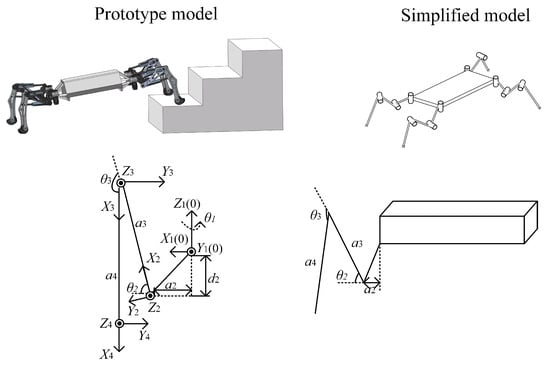
Figure 1. D-H coordinate system of the single-leg structure of the prototype and the simplified model.

Figure 1 shows the D-H coordinate system of the single-leg structure, where $a_2$ = 98.5 mm, $a_3$ = 350 mm, $a_4$ = 420 mm, and $d_2$ = 152 mm; and the circle represents the vector facing outward from the vertical paper.

The D-H parameter table of the leg is shown in Table 2:

Table 2. D-H parameterTable.

i	${\mathit{a}}_{\mathit{i}}$/mm	${\mathit{\alpha }}_{\mathit{i}}$/rad	${\mathit{d}}_{\mathit{i}}$/mm	${\mathit{\theta }}_{\mathit{i}}$/rad	Range of ${\mathit{\theta }}_{\mathit{i}}$
1	$\theta$	0	0	${\theta }_1$	($-\pi$/2, $\pi$/2)
2	$a_2$	$\pi$/2	$d_2$	${\theta }_3$	(0, $\pi$/3)
3	$a_3$	0	0	${\theta }_3$	($-\pi$/6, $-5\pi$/6)
4	$a_4$	0	0	0	(0, 0)

All the symbols and abbreviations can be seen in the Abbreviations section. By using the D-H parameters, the kinematic solution of the robot can be found.

Robotic inverse kinematics involves the calculation of joint-angle solutions with a known terminal pose [32]. The inverse solution results are:

$${\theta }_1=arctan\left(p_y,p_x\right)-arctan\left(0,1\right)$$

(1)

$${\theta }_2=arctan\left(a_3+a_{4}cos{\theta }_3,-a_{4}sin{\theta }_3\right)-arctan\left(K,\sqrt{{(a_3+a_{4}cos{\theta }_3)}^2+{(-a_{4}sin{\theta }_3)}^2-K^2}\right)$$

(2)

where $K=\frac{cos{\theta }_1}{{cos}^2{\theta }_1-{sin}^2{\theta }_1}{p}_x-\frac{sin{\theta }_1}{{cos}^2{\theta }_1-{sin}^2{\theta }_1}{p}_y-a_2$.

$${\theta }_3=-arccos\left(\frac{-{\left(p_{x}cos{\theta }_1-68.5\right)}^2-{\left(p_{y}sin{\theta }_1\right)}^2-{\left(p_z+152\right)}^2+a_3^2+a_4^2}{2a_3{a}_4}\right)$$

(3)

2.2. A Penalty Function That Optimizes the Limit of the Angular Velocity

The goal of trajectory planning for the robot is to generate a suitable joint motion rule ${\varphi }_t$ without violating the additional constraints to complete the task. In this paper, a 3-3-5 mixed polynomial algorithm (3-3-5 algorithm) is used to fit robot trajectory [33].

To realize the constraint on the angular velocity of each joint of the robot in the algorithm and reduce the impact on the motor, a penalty function is introduced to limit the maximum angular velocity of each joint. Additionally, in the case of the penalty function introduced in this paper, the joint motion law ${\varphi }_t$ can be represented as a fitness function that satisfies the inequality constraint and the equation constraint. ZHENG K M et al. [34] adopted a penalty function to take maximum torque as a constraint condition and ensured that the trajectory of each joint of the manipulator was within a safe range by introducing a penalty function.

To ensure that the running speed of each joint of the robot does not exceed the speed limit, we set the maximum angular velocity Vmax for each joint. Since this robot hardware can support a maximum motor speed of 25°/s, to ensure safety, the speed limit was set to 20°/s, which is $V_{max}$ = 0.349 rad/s. By introducing the penalty function, the maximum speed of each joint is restricted to the speed limit. The penalty function formula is as follows:

$$\left\{\begin{array}{c}minf\left(t\right),t\in A\\ A\subseteq \left\{\left.t\right|\left|{\phi }_j\left(t\right)\right|\le {\phi }_{max}\right\}\end{array}\right.$$

(4)

where ${\phi }_j\left(t\right)\le {\phi }_{max}$, and $j=1,2,3\dots \dots m$ is a constraint, which can be rewritten as $\left|{\phi }_j\left(t\right)\right|-{\phi }_{max}\le 0$ and is equal to $max\left[\left|{\phi }_j\left(t\right)\right|-{\phi }_{max},0\right]=0$. The updated fitness function formula is obtained as follows:

$$F\left(t\right)=f\left(t\right)+M{G}_j\left(t\right)$$

(5)

where $F\left(t\right)$ is the updated time-dependent fitness function; $G_j\left(t\right)={\displaystyle \sum _{j=1}^m}max\left[\left|{\phi }_j\left(t\right)\right|-{\phi }_{max},0\right]$; and M is the penalty factor, which must be a large nonnegative integer. Using a particularly large penalty factor M is consistent with the result obtained by taking a relatively small penalty factor [35]. The penalty function algorithm is shown in Algorithm 1:

Algorithm 1 Plenty function.

Input: $V_{max}$, M, ${\phi }_j\left(t\right)$, $t_1$, $t_2$, $t_3$ Output: $Fitness$ 1: $fitness=t_1+t_2+t_3$ 2: if ${\phi }_j\left(t\right)>{\phi }_{max}$ then 3:     $max[{\phi }_j\left(t\right)-{\phi }_{max},0]$ 4:     $G_j\left(t\right)=$${\sum }_{j=1}^9$$max[{\phi }_j\left(t\right)-{\phi }_{max},0]$ 5:     $Fitness=fitness+M{G}_j\left(t\right)$ //M is penalty factor 6: else 7:     Accept current value ${\phi }_j\left(t\right)$ 8: end if

3. Brief Introduction to the Whale Optimization Algorithm

The whale optimization algorithm is a new type of bionic intelligent optimization algorithm, proposed by Mirjalili and Lewis [36] in 2016. The algorithm simulates the bubble net feeding behavior of whales. When whales detect the location of the target, they produce spiral-shaped bubbles that surround the prey and move along the bubbles. The WOA process can be divided into three parts: encircling prey, foaming attack, and random searching. Given the issue that the convergence speed of the WOA cannot adjusted, and it converges too fast, the adaptive weight is introduced into the WOA to balance the exploration and exploitation ability of the algorithm.

3.1. Encircling Prey

In the whale optimization algorithm, assuming that the optimal position in the current population is prey, and the other whale individuals in the population are close to the optimal individual, and each position is updated according to the optimization rules, the mathematical expression is:

$$D=\left|C\ast X^{{}^{\prime }}\left(t\right)-X\left(t\right)\right|$$

(6)

$$X(t+1)=X^{{}^{\prime }}\left(t\right)-A\ast D$$

(7)

where t is the number of iterations, $X^{{}^{\prime }}$ is the current optimal solution position of the population (target position), X is the whale position, and D is the distance between the target location and the whale position. The expressions for A and C are as follows:

$$A=2a\ast ran{d}_1-a$$

(8)

$$C=2\ast ran{d}_2$$

(9)

where $rand$ is a random number between [0, 1] and a is the convergence factor, which decreases linearly from 2 to 0 as the number of iterations increases. The advantage of defining a like this is to make individuals gradually converge to target, which meets the requirements of encircling prey.

3.2. Bubble-Net Attacking Method

During the hunt, the whale approaches the prey in a spiral path and sends out bubbles to attack. To describe the mathematical model of the process, shrinking the encircling mechanism and spiral updating of the position are introduced to describe it.

3.2.1. Shrinking Encircling Mechanism

The shrinkage encircling mechanism reflects the local search aspect of the algorithm, which is achieved by reducing the value of a. If A is in the interval [−1, 1], the whale, after the updated position, is restricted to the current position and the prey position, thereby achieving the encirclement of the prey.

Figure 2 shows the possible positions from $\left(X,Y\right)$ toward ($X^{{}^{\prime }}$,$Y^{{}^{\prime }}$), which can be achieved by $0\le A\le 1$ in a 2D space.

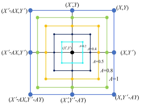
Figure 2. Shrinking encircling mechanism ($X^{{}^{\prime }}$ is the current optimal solution).

3.2.2. Spiral Updating of Position

As shown in Figure 2, to simulate the spiral updating of position, it is necessary to first calculate the distance between each whale $\left(X,Y\right)$ and the prey ($X^{{}^{\prime }}$,$Y^{{}^{\prime }}$) and then simulate the way the whale moves by using a spiral mathematical model, which is modeled as follows:

$$X(t+1)=D^{\ast }\ast e^{bl}\ast cos\left(2\pi l\right)+X^{{}^{\prime }}\left(t\right)$$

(10)

where $D^{\ast }=\left|X^{{}^{\prime }}\left(t\right)-X\left(t\right)\right|$ is the distance between the individual and the current optimal position; b is the logarithmic helix shape constant; l is a random number on [−1, 1]. As shown in Figure 3, the whales swim alongside their prey within a shrinking circle while swimming in spiral paths. To model this behavior, assume that the probability of choosing between shrinkage enveloping mechanisms or spiral update locations is 50%. The mathematical model for the position updating of the whale optimization algorithm is shown in Equation (11).

$$X(t+1)=\left\{\begin{array}{c}\begin{array}{cc}{X}^{{}^{\prime }}\left(t\right)-A\ast D& P<0.5\end{array}\\ \begin{array}{cc}{D}^{\ast }\ast e^{bl}\ast cos\left(2\pi l\right)+X^{{}^{\prime }}\left(t\right)& P\ge 0.5\end{array}\end{array}\right.$$

(11)

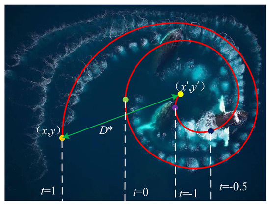
Figure 3. Process of spiral updating of position.

3.2.3. Search for Prey

In fact, whales search randomly based on each other’s location. Therefore, the process is represented by the random variable A. If A is beyond the range of [−1, 1], the whale is far away from the current optimal individual and updates its own position according to others’ positions. The mathematical model is as follows.

$$D=\left|C\ast X_{\mathrm{rand}}-X\right|$$

(12)

$$X(t+1)=X_{rand}-A\ast D$$

(13)

where $X_{rand}$ is the position of a random individual in the current population.

4. Hybrid Improved-Whale-Optimization–Simulated-Annealing Algorithm

The traditional polynomial-interpolation trajectory-planning algorithm requires setting conditions such as time velocity and acceleration at the interpolation point before planning, so time optimization cannot be achieved [7]. To address the above problems, we propose an improved IWOA-SA algorithm to optimize the trajectory generated by the 3-3-5 polynomial interpolation algorithm based on time optimization. By introducing adaptive weights, the exploration and exploitation capabilities of the algorithm are balanced and combined with the simulated annealing algorithm, and the problem of easily falling into a local optimum is avoided.

The introduction of SA into the WOA is a combination of the solid annealing principle and bionics. The main idea is to put randomness into the process of the WOA iteration; at the same time, this kind of randomness has to converge in the final stage of iteration; otherwise, the whole algorithm will be in a divergent state. ELHOSSEINI M A [29] set an adaptive random parameter C, but its convergence ability is relatively small. In addition, whether this kind of algorithm can fall into a local optimum is not proven.

4.1. Improved Whale Optimization Algorithm

To balance the exploration and exploitation ability of the WOA, adaptive weights are introduced. The adaptive weight formula is shown in Equation (11).

$$w=e^{-{\left(\frac{t}{t_{max}}\right)}^3}$$

(14)

When the maximum number of iterations is 100, and the adaptive weight curve is shown in Figure 4:

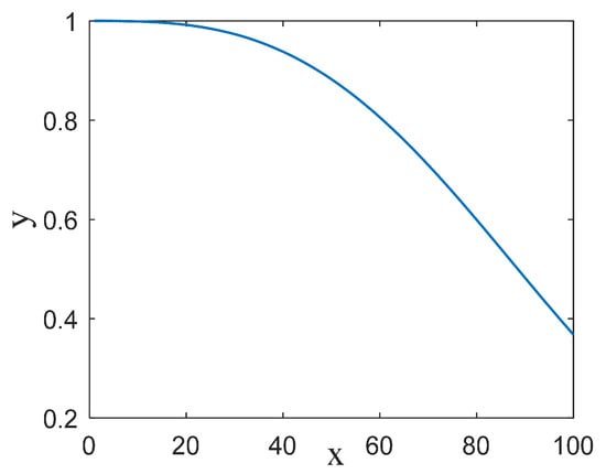
Figure 4. Function curve of $y=e^{-{\left(\frac{x}{100}\right)}^3}$.

As shown in Figure 4, in the initial stage of the iteration, the weight is larger and the slope is smaller, guaranteeing an appropriate search range; in the end stage, the weight is smaller and the slope is larger, which improves the optimization ability of the algorithm and accelerates the convergence speed. It also balances the exploration and exploitation ability of the algorithm. After adopting the adaptive weight, the mathematical model for the position update of the whale optimization algorithm is shown in Equation (15).

$$X(t+1)=\left\{\begin{array}{c}\begin{array}{cc}w\ast X^{{}^{\prime }}\left(t\right)-A\ast D& P<0.5\end{array}\\ \begin{array}{cc}{D}^{\ast }\ast e^{bl}\ast cos\left(2\pi l\right)+w\ast X^{{}^{\prime }}\left(t\right)& P\ge 0.5\end{array}\end{array}\right.$$

(15)

4.2. Simulated Annealing Algorithm

The simulated annealing algorithm (SA) was first proposed in 1953 by N Metropolis. S Kirkpatrick introduced the idea of annealing into the field of combinatorial optimization in 1983 [37]. The Metropolis acceptance criterion was integrated into the SA algorithm. The Metropolis criterion is used to describe the equilibrium set of atoms at a particular temperature and is able to accept higher energies with a certain probability [38].

The algorithm idea of SA algorithm is as follows: start cooling from a high initial temperature $T_k$, make $T_{K+1}=\delta \times T_K$ gradually lower the temperature and search at each temperature. It accepts a solution worse than the current one with probability p in each round of searching until temperature equilibrium is reached. The acceptance probabilities used in this article are:

$$p=\left\{\begin{array}{c}\begin{array}{cc}1,& f\left(x_0^{\ast }\right)\le f\left(x_0\right)\end{array}\\ \begin{array}{cc}{e}^{-\Delta f/T},& Otherwise\end{array}\end{array}\right.$$

(16)

where f is the fitness function.

$x_0^{\ast }$ is the position of the new particle spawned near $x_0$; if $f\left(x_0^{\ast }\right)$ is less than $f\left(x_0\right)$, the new solution a is accepted (probability is 1), and update the velocity and position of the particle; if $f\left(x_0^{\ast }\right)$ is greater than $f\left(x_0\right)$, it means that $x_0^{\ast }$ deviates further from the global optimal value. At this point, the algorithm does not immediately discard the new solution but determines it based on the acceptance probability p.

In the case of a high initial temperature, the probability of an inferior solution being accepted is larger, and with a decreasing temperature, the probability of accepting an inferior solution gradually decreases.

4.3. Hybrid Improved-Whale-Optimization–Simulated-Annealing Algorithm

In this paper, on the basis of inheriting the advantages of the WOA, the simulated annealing mechanism is introduced. In each update iteration, the Metropolis criterion is used to accept the better solution while accepting the worse solution with a certain probability, which makes the WOA jump out of the local optimization.

The global optimal position obtained in the SA algorithm is used to replace the global optimal position in the WOA, and the position-update equation after replacement is as shown in Equations (17)–(19):

$$D=\left|C\ast Leade{r}_{pos}-X\left(t\right)\right|$$

(17)

$$D^{\ast }=\left|Leade{r}_{pos}-X\left(t\right)\right|$$

(18)

$$X\left(t+1\right)=\left\{\begin{array}{c}\begin{array}{cc}w\ast Leade{r}_{pos}-A\ast D& P<0.5\end{array}\\ \begin{array}{cc}{D}^{\ast }\ast e^{bl}\ast cos\left(2\pi l\right)+w\ast Leade{r}_{pos}& P\ge 0.5\end{array}\end{array}\right.$$

(19)

If the initial temperature $T_k$ is high enough, the high-quality solution can be obtained, but the running time will be too long. If $T_k$ is too small, it will affect the quality of the solution; therefore, one should choose a reasonable $T_k$ and cooling coefficient $\delta$. The value of the $\delta$ is between 0.4 and 0.99 [39].

Referring to the work done by P J van Laarhoven [40] and Yang Dan et al. [39], the initial temperature $T_k$ in this paper is shown in Equation (20):

$$T_k=\frac{F\left(p_g^0\right)}{ln\left({\chi }_0^{-1}\right)}$$

(20)

where $F\left(p_g^0\right)$ is the fitness value corresponding to the global optimal position obtained by the IWOA-SA algorithm population initialization, and ${\chi }_0$ takes a value of approximately one, which is the initial acceptance rate of the new solution. The main loop of the IWOA-SA algorithm is shown in Algorithm 2.

As shown in Algorithm 2, the combination of the SA algorithm with the improved WOA can give the randomness of the WOA, making it not just a simple hillclimber. As we can see from Step 7, we first compare the current optimal solution with $fitness\left(x_i\left(t\right)\right)$ ($x_i\left(t\right)$ is a random unit in SA algorithm). When the current best solution is better than the $fitness\left(x_i\left(t\right)\right)$, we do not just accept the solution. Instead, we calculate the probability p and compare it with a random number between 0 and 1 and accept a new value near $x_i\left(t\right)$ (can see from the Step 11 to 14), and we take the new value $Leade{r}_{pos}$ into the WOA. By this method, we successfully add the randomness into the proposed algorithm; as a result, the proposed algorithm can jump out of the local optimum.

Algorithm 2 IWOA-SA main loop.

Input: $Dim$, $t_{max}$, $NP$//space dimensionality; iteration number; population number Output: $X^{\ast }\left(t\right)$ // global best position vector   $fgb=fitness\left(p_g\right)$ //$p_g$ is current optimal position vector 2: $fx=fitness\left(x_i\left(t\right)\right)$   $T_k=fitness\left(p_g\right)/ln\left(1.5\right)$ 4: $t=0$//initialization   while t < $t_{max}$ do 6:     for i = 1 to $NP$ do             if $fx$ < $fgb$ then //Compare with current optimal solution 8:                 $p_g=x_i\left(t\right)$                  $fgb=fx$ 10:          else                   p = e$(fitness\left(p_g\right)-fitness\left(y_i\left(t\right)\right))/T_k$ // accept $y_i\left(t\right)$ with accept rate p 12:               if rand(0, 1) < p then                         $p_g=y_i\left(t\right)$ // $y_i\left(t\right)$ is a new value near $x_i\left(t\right)$ in SA algorithm 14:                     $fgb=fitness\left(y_i\left(t\right)\right)$                  end if 16:          end if        end for 18:     $Leade{r}_{pos}=p_g$        for i = 1 to $NP$ do 20:         $a=2-t\ast (2/t_{max})$//a decreases linearly fron 2 to 0            $a_2=-1+t\ast ((-1)/t_{max})$//$a_2$ linearly dicreases from −1 to −2 22:         $A=2\ast a\ast rand(0,1)-a$            $C=2\ast rand(0,1)$ 24:         $l=(a_2-1)\ast rand(0,1)+1$            if P < 0.5 then 26:               if $\left|A\right|\ge 1$ then                      $D=|C.X_{rand}-X\left(t\right)|$ 28:                   $X^{\ast }(t+1)=X_{rand}-A.D$                  else if $\left|A\right|<1$ then 30:                   $D=|C.Leade{r}_{pos}-X\left(t\right)|$                     $X^{\ast }(t+1)=w.Leade{r}_{pos}-A.D$ 32:                end if             else if $P\ge 0.5$ then 34:                $D^{\ast }=|Leade{r}_{pos}-X\left(t\right)|$                   $X^{\ast }(t+1)=D^{\ast }.$e${}^{bl}.cos\left(2\pi l\right)+w.Leade{r}_{pos}$ 36:         end if       end for 38:     $T_{k+1}=T_k\ast \delta$//Annealing operation, $\delta$ is the attenuation factor of the SA algorithm        $t=t+1$ 40: end while

4.4. Convergence Proof of the IWOA-SA Algorithm

The probability-measure method can be used to prove the global convergence of IWOA-SA. According to the global convergence criterion and theorem [41], to prove that the algorithm can converge into the global optimum, the algorithm needs to meet the following two conditions:

 Theorem 1.

$f\left(W\right(x,\zeta \left)\right)\le f\left(x\right)$ and if $\zeta \in S$, then $f\left(W\right(x,\zeta \left)\right)\le f\left(\zeta \right)$

where f is fitness function, W is the algorithm, and x is a point of the subset S of the solution space $R^N$, which can minimize the value of the function or produce an acceptable infimum of the function’s value on S. $\zeta$ is the solution searched in the iterative search of algorithm W.

 Theorem 2.

For any Borel subset A in S, have:

$$\prod _{k=0}^{\infty }(1-{\mu }_k\left(A\right))=0$$

(21)

where ${\mu }_k\left(A\right)=P(x^k\in A|x^0,x^1,\dots x^{k-1})$ is the probability measure of the result of the kth iteration of algorithm W on the set A. The significance of this assumption is, for subset A in S, after infinite iterations of the algorithm, it is impossible to miss the solution space S of any Borel subset A; that is, the probability that an algorithm which satisfies the condition does not search for an approximate global optimum for an infinite number of consecutive iterations is zero.

 Corollary 1

(Global Search [41]). Suppose that f is a measurable function, S is a measurable subset of $R^N$, and Theorem 1 Theorem 2 are satisfied. ${\left\{x_k\right\}}_{k=1}^{\infty }$ is a sequence generated by the algorithm. Then:

$$\underset{k\to \infty }{lim}P\left[x^k\in R\right]=1$$

(22)

where R is the global optimal set, and $P\left[x^k\in R\right]$ is the probability that the result of the kth generation of the algorithm falls in R.

Proof of Theorem 1. 

According to description of IWOA-SA, define D as:

$$W(G_t,X_t^i)=\left\{\begin{array}{c}\begin{array}{cc}{G}_t& f\left(g\left(X_t^i\right)\right)\ge f\left(G_t\right)\end{array}\\ \begin{array}{cc}g\left(X_t^i\right)& f\left(g\left(X_t^i\right)\right)<f\left(G_t\right)\end{array}\end{array}\right.$$

(23)

where $g\left(X_t^i\right)$ represents the position of whale individual i after the tth update after the second interpolation operation and $G_t$ is the location of the current global optimal solution. The SA annealing process shows that at the end stage of the algorithm, the probability of accepting a worse solution is very small; as a result, the value of the fitness function is monotonic and does not increase. In addition, it gradually converges to the infimum of the solution space. □

Proof of Theorem 2. 

Suppose that the individual i of the IWOA-SA algorithm in discrete space in time t has $X_i^{\left(t\right)}=x_i^t$, $x_i^t\in B$, B is state space, $x_i^t$ is the state of individual i at time t. The sequence $\{X_i^{\left(t\right)},t\ge 1\}$ of state $X_i^{\left(t\right)}$ is a discrete random variable in discrete space. We can see from the population update formula (15) of IWOA-SA, the current individual state is only related to the state of the previous moment and has no connection with the number of present iterations; therefore, sequence $\{X_i^{\left(t\right)},t\ge 1\}$ is a homogeneous Markov chain.

Assuming that the individual i of IWOA-SA falls into local optimal state $h^{\left(t\right)}$ in time t, the one-step transfer probability of population sequence $\{X_i^{\left(t\right)},t\ge 1\}$ is:

$$P\{X_i^{(t+1)}=h^{(t+1)}|X_i^{\left(t\right)}=h^{\left(t\right)}\}=P\{X_i^{(t+1)}=w\ast L\left(t\right)-A\left|C\ast L\left(t\right)-X_i^{\left(t\right)}\right||X_i^{\left(t\right)}=h^{\left(t\right)}\}=\left\{\begin{array}{c}\begin{array}{cc}1& w\ast L\left(t\right)=h^{\left(t\right)}\mathrm{and}A=0\end{array}\\ \begin{array}{cc}0& otherwise\end{array}\end{array}\right.$$

(24)

where $L\left(t\right)$ is the optimal solution after SA replacement. Due to the parameter A in this paper not being zero, the IWOA-SA algorithm does not easily fall into local optima.

Set B as a Borel subset in solution space S. If individual i of IWOA-SA cannot be involved in disaggregation B at iteration time t, there will be:

$$P\{X_i^{\left(t\right)}\notin B\}=P\{X_i^{\left(t\right)}\notin B|X_i^{(t-1)}\in B\}\ast P\{X_i^{(t-1)}\in B\}+P\{X_i^{\left(t\right)}\notin B|X_i^{(t-1)}\notin B\}\ast P\{X_i^{(t-1)}\notin B\}$$

(25)

As IWOA-SA is an absorbing Markov process, as a result, $P\{X_i^{\left(t\right)}\notin B|X_i^{(t-1)}\in B\}=0$, so Equation (25) can be transformed into:

$$P\{X_i^{\left(t\right)}\notin B\}=P\{X_i^{\left(t\right)}\notin B|X_i^{(t-1)}\notin B\}\ast P\{X_i^{(t-1)}\notin B\}$$

(26)

It is known from the one-step transfer probability of IWOA-SA that it cannot fall into a local optimum; as a result, individual i will reach the globally optimal solution with a certain probability in the iteration process, which is:

$$0<P\{X_i^{\left(t\right)}\in B|X_i^{(t-1)}\notin B\}<1$$

(27)

Equation (26) can be changed into:

$$P\{X_i^{\left(t\right)}\notin B\}=\{1-P\{X_i^{\left(t\right)}\in B|X_i^{(t-1)}\notin B\}\}\ast P\{X_i^{(t-1)}\notin B\}$$

(28)

As a result:

$$P\{X_i^{\left(t\right)}\notin B\}=\prod _{k=0}^t\{1-P\{X_i^{\left(k\right)}\in B|X_i^{\left(k\right)}\notin B\}\}\ast P\{X_i^{\left(0\right)}\notin B\}$$

(29)

As $0<P\{X_i^{\left(t\right)}\in B|X_i^{(t-1)}\notin B\}<1$, when the number of iterations tends to infinity, there will be:

$$\prod _{k=0}^{\infty }\{1-P\{X_i^{\left(k\right)}\in B|X_i^{(k-1)}\notin B\}\}=0$$

(30)

Therefore, $\prod _{k=0}^{\infty }P\{X_i^{\left(t\right)}\notin H^{\ast }\}=0$, which is $\prod _{k=0}^{\infty }(1-{\mu }_k\left(B\right))=0$.

Certification established. □

As the result, we can know from the Corollary 1 that IWOA-SA has global convergence.

5. Experimental Verification

To verify the feasibility of the method, six unconstrained optimization problems were solved by simulation, and the trajectory generated by the 3-3-5 mixed polynomial interpolation equation (Appendix A) was optimized by the proposed optimization algorithm. The IWOA-SA algorithm and the WOA, PSO, and GWO algorithms used for comparative analysis were programmed by MATLAB R2017b. The global optimal solution obtained by optimization was used to evaluate the effectiveness and stability of IWOA-SA, and the average (MEAN) and standard deviation (STD) of the optimal solution were used as the evaluation statistics. The formula is shown in (31) and (32):

$$MEAN=\frac{1}{N}\sum _{i=1}^N{f}_i^{best}$$

(31)

$$STD=\sqrt{\frac{1}{N}\sum _{i=1}^N{(f_i^{best}-MEAN)}^2}$$

(32)

where $f_i^{best}$ is the optimal solution obtained in the ith operation, and N is the number of runs. The smaller the values of the mean and the standard deviation are, the more reliable and stable the solution provided by the algorithm [42].

5.1. Validate the Algorithm by Testing Functions

Six classical unconstrained optimization functions include the unimodal function ($F_1$-$F_2$), fixed-dimensional peak function ($F_3$-$F_4$), and variable-dimensional peak function ($F_5$-$F_6$). The details of the test function are shown in Table 3. There is only one optimal solution in the unimodal function to evaluate the convergence speed and exploitation ability of the algorithm. However, there is a global optimal solution in the multipeak function, which contains several local optimal solutions to evaluate the exploration ability of the algorithm. Each algorithm ran 10 times, the number of populations was set to 100, and the number of iterations was set to 600. The inertial weight of PSO was set to 0.8, and the learning factor was 1.5. The subpopulation of NHWOA was set to 4.

Table 3. Details of the test functions.

Functions	Dim	Range	Min
$F_1\left(x\right)={\displaystyle \sum _{i=1}^n}{x}_i^2$	30	$\left[-100,100\right]$	0
$F_2\left(x\right)={\displaystyle \sum _{i=1}^n}i{x}_i^4+rand[0,1)$	30	$\left[-1.28,1.28\right]$	0
$F_3\left(x\right)=4x_1^2-2.1x_1^4+\frac{1}{3}{x}_1^6+x_1{x}_2-4x_2^2+4x_2^4$	2	$\left[-5,5\right]$	−1.0316
$$\begin{gathered} F_4\left(x\right)=[1+{(x_1+x_2+1)}^2(19-14x_1+3x_1^2-14x_2+6x_1{x}_2+3x_2^2)]\times \\ [30+{(2x_1-3x_2)}^2\times (18-32x_1+12x_1^2+48x_2-36x_1{x}_2+27x_2^2)] \end{gathered}$$	2	$\left[-2,2\right]$	3
$F_5\left(x\right)={\displaystyle \sum _{i=1}^n}-x_{i}sin\left(\sqrt{x_i}\right)$	30	$\left[-500,500\right]$	−12,569.5
$F_6\left(x\right)={\displaystyle \sum _{i=1}^n}[x_{{}_i}^2-10cos\left(2\pi x_i\right)+10]$	30	$\left[-5.12,5.12\right]$	0

Table 4 shows that the IWOA-SA algorithm has advantages in global searching, can effectively avoid falling into a local optimum, and has better performance under the unimodal function (the mean value was the lowest and was the most stable one among six algorithms) and the variable-dimensional peak function (the mean value was lowest, about 33.6% lower than that of WOA-LFDE, and the stability was 38.2% higher than that of WOA; it was the most stable algorithm among six algorithms). The proposed algorithm has higher stability compared with WOA and GWO under fixed-dimensional peak functions. Our algorithm performed better in this experiment and demonstrated greater stability than the other algorithms. Therefore, the IWOA-SA effectively balances exploration and exploitation abilities.

Table 4. Comparison of test-function results.

		WOA	IWOA-SA	GWO	PSO	WOA-LFDE	NHWOA
$F_1$	MEAN	0	0	0	0.0247	0	0
	STD	0	0	0	0.0151	0	0
$F_2$	MEAN	$2.33\times {10}^{-3}$	$5.59\times {10}^{-5}$	$1.69\times {10}^{-3}$	0.456	6.41 × ${10}^{-3}$	1.22 × ${10}^{-2}$
	STD	3.16 × ${10}^{-3}$	$6.08\times {10}^{-5}$	0.79 × ${10}^{-3}$	0.249	2.36 × ${10}^{-3}$	7.97 × ${10}^{-3}$
$F_3$	MEAN	−1.0316	−1.0316	−1.0316	−1.0316	−1.0316	−1.0316
	STD	0	0	0	0	0	0
$F_4$	MEAN	3	3	3	3	3	3
	STD	2.41 × ${10}^{-5}$	0	$1.61\times {10}^{-5}$	0	0	0
$F_5$	MEAN	−1.12 ×${10}^4$	−1.16 ×${10}^4$	−5.71 ×${10}^3$	−6.73 ×${10}^3$	−7.708 ×${10}^3$	−6.17 ×${10}^3$
	STD	1.42 × ${10}^3$	3.21 × ${10}^2$	8.78 × ${10}^2$	7.25 × ${10}^2$	360.45	420.1
$F_6$	MEAN	0	0	1.2754	55.8276	32.23	47.75
	STD	0	0	2.7224	13.6437	8.0591	23.503

In Figure 5, the convergence curves of IWOA-SA, WOA, GWO, PSO, WOA-LFDE [43] and NHWOA [44] are compared. The “average” denotes the average of 10 runs. The WOA has advantages in local searching, but it easily falls into local optima. The GWO algorithm had good search performance for low-dimensional functions but poor search ability for high-dimensional functions. The optimization abilities of the PSO, WOA-LFDE, and NHWOA under the variable-dimensional peak function were poor, and they needed to be iterated more times to reach the optimal solution. Compared with the other five algorithms, the IWOA-SA algorithm converged quickly and could always obtain the best results among all six algorithms.

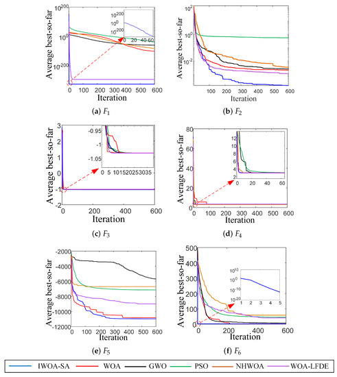
Figure 5. Convergence curves of the IWOA-SA, WOA, GWO, and PSO algorithms. (a) F1, (b) F2, (c) F3, (d) F4, (e) F5, (f) F6.

5.2. IWOA-SA Solves the Problem of Time-Optimal Trajectory Planning

The trajectory planning of the quadruped robot mentioned above was carried out, and the interpolation points selected in the experiment are shown in Table 5. At the same time, considering the actual situation of the robot, the maximum angular velocity of the joint was set to 20°/s through a penalty function. For all algorithms, the number of populations was 100, the number of iterations was 200, and each algorithm ran 10 times.

Table 5. Interpolation points selected in the experiment.

	Interpolation Point 1	Interpolation Point 2	Interpolation Point 3	Interpolation Point 4
Joint 1	0	0	0	0
Joint 2	−0.888	−0.90	−1.1545	−1.4122
Joint 3	2.527	2.4	1.5027	1.00659

The comparison of the optimization results of IWOA-SA, WOA, GWO, PSO, WOA-LFDE, and NHWOA are shown in Table 6.

Table 6. Comparison of experimental results of trajectory planning.

	WOA	IWOA-SA	GWO	PSO	NHWOA	WOA-LFDE
MEAN (S)	7.58	6.745	7.592	6.825	6.819	7.015
STD (S)	0.034	0.0167	0.00273	0.0208	0.0184	0.0179

Table 6 shows that the average time taken to reach the optimal solution by IWOA-SA was the smallest (over 10 runs), which shows that the IWOA-SA algorithm has strong optimization ability and is more stable than the others.

To verify whether the time taken by IWOA-SA is significantly different from that of the other five algorithms, we used the Kruskal–Wallis test. The $KW$ statistic can be tested using a chi-square distribution.

$$KW=\frac{12}{\mathrm{n}\ast (n+1)}\sum _{i=1}^K\frac{R_i^2}{n_i}-3\ast (n+1)$$

(33)

If there are knot values in the sample (number of data with the same rank value), the correction factor C is:

$$C=1-\frac{\sum ({\tau }_i^3-{\tau }_i)}{n^3-n}$$

(34)

Therefore, the expression for the sample statistic $K{W}_C$ is:

$$K{W}_C=\frac{KW}{C}$$

(35)

In cases of large samples, $n_i>5$, the larger is n, the more $KW$ approximately obeys the cardinal distribution with degrees of freedom $K-1$ under the null hypothesis, so the $KW$ statistic can be tested using the cardinal distribution. Assumptions:

 H0:

There was no significant difference in the running times obtained by the six algorithms;

 H1:

There was a significant difference in the running times obtained by the six algorithms.

After bringing in the parameters of this paper for calculation, $KW$ = 45.3268 and $K{W}_C$ = 45.431.

By checking the chi-square test table, the chi-square value was 12.833 for the degrees of freedom of $K-1=5$ and a significance level of 0.05. $K{W}_C>5.9915$. Therefore, the original hypothesis was rejected, and the six data groups were considered to be significantly different.

In Figure 6, the motion curves of each joint of the robot before and after optimization by the IWOA-SA algorithm are compared.

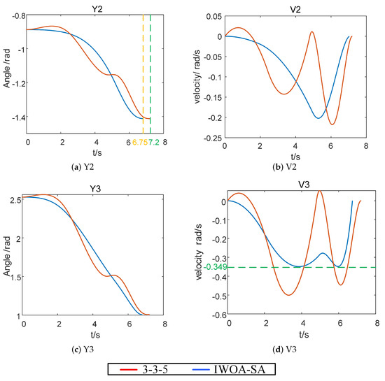
Figure 6. Running curve of each joint after using the optimization algorithm. (a) Y2, (b) V2, (c) Y3, (d) V3.

Table 7 shows the joint running-time comparison before and after using the optimization algorithm.

Table 7. Time comparison before and after using the optimization algorithm.

	Time (s)
3-3-5	7.2
IWOA-SA	6.745

In Table 7 and Figure 6, we can see that: (1) The IWOA-SA algorithm ensures that the angular velocity of each joint is within the velocity limit ($\pm 0.349$ rad/s). (2) The running time of each joint is reduced by about 6.25% compared with the 3-3-5 algorithm. As shown in Figure 6d, before using the optimization algorithm, the angular velocity of each joint of the robot easily exceeds the speed limit, and after using the optimization algorithm, the angular velocity of each joint is limited to the velocity range. Figure 7 shows the foot-end trajectory curve after using the IWOA-SA optimization algorithm.

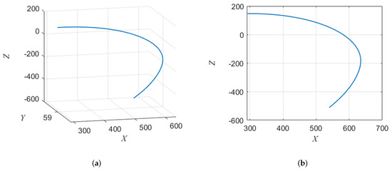
Figure 7. Foot-end trajectory curve. (a) Foot-end trajectory curve, (b) Trajectory curve in two-dimensional plane.

Figure 7 illustrates that when simulating a downstairs process, a retraction can be observed at the end of the foot-end trajectory curve, which effectively reduces the landing impact during touchdown. upon touchdown.

6. Conclusions

In this paper, an IWOA-SA algorithm was proposed to achieve the optimal time movement of the quadruped robot. The proposed algorithm adopts the simulated annealing mechanism of the SA algorithm to “jump” out of the local optima of the WOA. Adaptive weights were also introduced to balance the exploration and exploitation capabilities of the algorithm. To solve the time-optimal trajectory planning problem under certain kinematic constraints, we introduced a penalty function to transform unconstrained optimization problems into constrained optimization problems. Using Markov chains of stochastic process theory, we proved that our algorithm converges to the global optimal value as the number of iterations approaches infinity. Simulation results demonstrated the effectiveness of our method and the correctness of our theoretical analysis. Compared to other mainstream algorithms, our IWOA-SA algorithm performs better, being on average 33.6% better than the WOA-LFDE and having 38.2% higher stability than the WOA.

Additionally, our algorithm always constrains the angular velocity of each joint within the range of kinematic constraints, reducing joint running time by 6.25%. Our method can be effectively applied to the robot trajectory planning field, and future research will focus on extending IWOA-SA to optimize other trajectory models and address the dynamical problems of quadruped robots, such as the shifting of the center of mass.

References

- Li, X.; Zhou, H.; Feng, H.; Zhang, S.; Fu, Y. Design and Experiments of a Novel Hydraulic Wheel-Legged Robot (WLR). In Proceedings of the 2018 IEEE/RSJ International Conference on Intelligent Robots and Systems (IROS), Madrid, Spain, 1–5 October 2018; pp. 3292–3297. [Google Scholar]
- Zeng, X.; Zhang, S.; Zhang, H.; Li, X.; Zhou, H.; Fu, Y. Leg Trajectory Planning for Quadruped Robots with High-Speed Trot Gait. Appl. Sci. 2019, 9, 1508. [Google Scholar] [CrossRef]
- Hwangbo, J.; Lee, J.; Dosovitskiy, A.; Bellicoso, D.; Tsounis, V.; Koltun, V.; Hutter, M. Learning agile and dynamic motor skills for legged robots. Sci. Robot. 2019, 4, eaau5872. [Google Scholar] [CrossRef]
- Kolter, J.Z.; Ng, A.Y. The Stanford LittleDog: A learning and rapid replanning approach to quadruped locomotion. Int. J. Robot. Res. 2011, 30, 150–174. [Google Scholar] [CrossRef]
- Basile, F.; Caccavale, F.; Chiacchio, P.; Coppola, J.; Curatella, C. Task-oriented motion planning for multi-arm robotic systems. Robot. -Comput.-Integr. Manuf. 2012, 28, 569–582. [Google Scholar] [CrossRef]
- Chen, C.; He, Y.Q.; Bu, C.G.; Han, J.D. Feasible trajectory generation for autonomous vehicles based on quartic Bézier curve. Zidonghua Xuebao/Acta Autom. Sin. 2015, 41, 486–496. [Google Scholar]
- Wang, M.; Luo, J.; Walter, U. Trajectory planning of free-floating space robot using Particle Swarm Optimization (PSO). Acta Astronaut. 2015, 112, 77–88. [Google Scholar] [CrossRef]
- Haddad, M.; Khalil, W.; Lehtihet, H.E. Trajectory Planning of Unicycle Mobile Robots with a Trapezoidal-Velocity Constraint. IEEE Trans. Robot. 2010, 26, 954–962. [Google Scholar] [CrossRef]
- Dinçer, Ü.; Çevik, M. Improved trajectory planning of an industrial parallel mechanism by a composite polynomial consisting of Bézier curves and cubic polynomials. Mech. Mach. Theory 2019, 132, 248–263. [Google Scholar] [CrossRef]
- Huang, Q.; Yokoi, K.; Kajita, S.; Kaneko, K.; Arai, H.; Koyachi, N.; Tanie, K. Planning walking patterns for a biped robot. IEEE Trans. Robot. Autom. 2001, 17, 280–289. [Google Scholar] [CrossRef]
- Xiong, C.; Chen, D.; Lu, D.; Zeng, Z.; Lian, L. Path planning of multiple autonomous marine vehicles for adaptive sampling using Voronoi-based ant colony optimization. Robot. Auton. Syst. 2019, 115, 90–103. [Google Scholar] [CrossRef]
- Srinivas, T.; Madhusudhan, A.K.K.; Manohar, L.; Stephen Pushpagiri, N.M.; Ramanathan, K.C.; Janardhanan, M.; Nielsen, I. Valkyrie—Design and Development of Gaits for Quadruped Robot Using Particle Swarm Optimization. Appl. Sci. 2021, 11, 7458. [Google Scholar] [CrossRef]
- Seo, J.H.; Im, C.H.; Kwak, S.Y.; Lee, C.G.; Jung, H.K. An Improved Particle Swarm Optimization Algorithm Mimicking Territorial Dispute Between Groups for Multimodal Function Optimization Problems. IEEE Trans. Magn. 2008, 44, 1046–1049. [Google Scholar] [CrossRef]
- Sharma, A.; Sharma, A.; Pandey, J.K.; Ram, M. Swarm Intelligence: Foundation, Principles, and Engineering Applications; CRC Press: Boca Raton, FL, USA, 2022. [Google Scholar]
- Mirjalili, S.; Mirjalili, S.M.; Lewis, A. Grey Wolf Optimizer. Adv. Eng. Softw. 2014, 69, 46–61. [Google Scholar] [CrossRef]
- Malyshev, D.; Cherkasov, V.; Rybak, L.; Diveev, A. Synthesis of Trajectory Planning Algorithms Using Evolutionary Optimization Algorithms. In Proceedings of the Advances in Optimization and Applications: 13th International Conference, OPTIMA 2022, Petrovac, Montenegro, 26–30 September 2022; Springer Nature: Cham, Switzerland, 2023; pp. 153–167. [Google Scholar]
- Husnain, G.; Anwar, S. An Intelligent Probabilistic Whale Optimization Algorithm (i-WOA) for Clustering in Vehicular Ad Hoc Networks. Int. J. Wirel. Inf. Netw. 2022, 29, 1–14. [Google Scholar]
- Nadimi-Shahraki, M.H.; Fatahi, A.; Zamani, H.; Mirjalili, S.; Oliva, D. Hybridizing of Whale and Moth-Flame Optimization Algorithms to Solve Diverse Scales of Optimal Power Flow Problem. Electronics 2022, 11, 831. [Google Scholar] [CrossRef]
- Nadimi-Shahraki, M.H.; Fatahi, A.; Zamani, H.; Mirjalili, S.; Abualigah, L. An Improved Moth-Flame Optimization Algorithm with Adaptation Mechanism to Solve Numerical and Mechanical Engineering Problems. Entropy 2021, 23, 1637. [Google Scholar] [CrossRef]
- Abualigah, L.; Al-Betar, M.A.; Mirjalili, S. Migration-Based Moth-Flame Optimization Algorithm. Processes 2021, 9, 2276. [Google Scholar]
- Zamani, H.; Nadimi-Shahraki, M.H.; Gandomi, A.H. Starling murmuration optimizer: A novel bio-inspired algorithm for global and engineering optimization. Comput. Methods Appl. Mech. Eng. 2022, 392, 114616. [Google Scholar] [CrossRef]
- Sharma, A.; Sharma, A.; Chowdary, V.; Srivastava, A.; Joshi, P. Cuckoo Search Algorithm: A Review of Recent Variants and Engineering Applications. In Metaheuristic and Evolutionary Computation: Algorithms and Applications; Springer Nature: Singapore, 2021; pp. 177–194. [Google Scholar]
- Grenko, T.; Šegota, S.B.; Anđelić, N.; Lorencin, I.; Štifanić, D.; Štifanić, J.; Car, Z. On the Use of a Genetic Algorithm for Determining Ho–Cook Coefficients in Continuous Path Planning of Industrial Robotic Manipulators. Machines 2023, 11, 167. [Google Scholar] [CrossRef]
- Nadimi-Shahraki, M.H.; Zamani, H.; Mirjalili, S. Enhanced whale optimization algorithm for medical feature selection: A COVID-19 case study. Comput. Biol. Med. 2022, 148, 105858. [Google Scholar] [CrossRef]
- Zamani, H.; Nadimi-Shahraki, M.H.; Gandomi, A.H. QANA: Quantum-based avian navigation optimizer algorithm. Eng. Appl. Artif. Intell. 2021, 104, 104314. [Google Scholar] [CrossRef]
- Zhang, H.; Wang, H.; Li, N.; Yu, Y.; Su, Z.; Liu, Y. Time-optimal memetic whale optimization algorithm for hypersonic vehicle reentry trajectory optimization with no-fly zones. Neural Comput. Appl. 2018, 32, 2735–2749. [Google Scholar] [CrossRef]
- Lv, H.; Feng, Z.; Wang, X.; Zhou, W.; Chen, B. Structural damage identification based on hybrid whale annealing algorithm and sparse regularization. J. Vib. Shock 2021, 40, 85–91. [Google Scholar]
- Wang, T.; Xin, Z.J.; Miao, H.; Zhang, H.; Chen, Z.Y.; Du, Y. Optimal Trajectory Planning of Grinding Robot Based on Improved Whale Optimization Algorithm. Math. Probl. Eng. 2020, 2020, 1–8. [Google Scholar] [CrossRef]
- El-Hosseini, M.A.; Haikal, A.Y.; Badawy, M.M.; Khashan, N. Biped robot stability based on an A-C parametric Whale Optimization Algorithm. J. Comput. Sci. 2019, 31, 17–32. [Google Scholar] [CrossRef]
- Locatelli, M. Convergence properties of simulated annealing for continuous global optimization. J. Appl. Probab. 1996, 33, 1127–1140. [Google Scholar] [CrossRef]
- Zhao, J.; Wang, H.; Liu, W.; Zhang, H. A learning-based multiscale modelling approach to real-time serial manipulator kinematics simulation. Neurocomputing 2020, 390, 280–293. [Google Scholar] [CrossRef]
- Zheng, C.; Su, Y.; Müller, P.C. Simple online smooth trajectory generations for industrial systems. Mechatronics 2009, 19, 571–576. [Google Scholar] [CrossRef]
- Xu, R.; Tian, J.; Zhai, X.; Li, J.; Zou, J. Research on Improved Hybrid Polynomial Interpolation Algorithm for Rail Inspection Robot. In Proceedings of the 2021 5th International Conference on Electronic Information Technology and Computer Engineering, Xiamen, China, 22–24 October 2021; Association for Computing Machinery: New York, NY, USA, 2022; pp. 1207–1213. [Google Scholar]
- Zheng, K.; Hu, Y.; Wu, B. Trajectory planning of multi-degree-of-freedom robot with coupling effect. J. Mech. Sci. Technol. 2019, 33, 413–421. [Google Scholar] [CrossRef]
- Si, C.Y.; Lan, T.; Hu, J.J.; Wang, L.; Wu, Q.D. Penalty parameter of the penalty function method. Control. Decis. 2014, 29, 1707–1710. [Google Scholar]
- Mirjalili, S.; Lewis, A. The Whale Optimization Algorithm. Adv. Eng. Softw. 2016, 95, 51–67. [Google Scholar] [CrossRef]
- Javidrad, F.; Nazari, M.H. A new hybrid particle swarm and simulated annealing stochastic optimization method. Appl. Soft Comput. 2017, 60, 634–654. [Google Scholar] [CrossRef]
- Borkar, V.S. Equation of State Calculations by Fast Computing Machines. Resonance 2022, 27, 1263–1269. [Google Scholar] [CrossRef]
- Yang, D.; Lu, T.; Guo, W.X.; Wang, X. MIT Image Reconstruction Method Based on Simulated Annealing Particle Swarm Algorithm. J. Northeast. Univ. 2021, 42, 531–537. [Google Scholar]
- Laarhoven, P.J.V.; Aarts, E.H.L. Simulated Annealing: Theory and Applications; Springer: Berlin/Heidelberg, Germany, 1987. [Google Scholar]
- Solis, F.J.; Wets, R.J.B. Minimization by Random Search Techniques. Math. Oper. Res. 1981, 6, 19–30. [Google Scholar] [CrossRef]
- Zhao, W.; Wang, L.; Mirjalili, S.M. Artificial hummingbird algorithm: A new bio-inspired optimizer with its engineering applications. Comput. Methods Appl. Mech. Eng. 2022, 388, 114194. [Google Scholar] [CrossRef]
- Liu, M.; Yao, X.; Li, Y. Hybrid whale optimization algorithm enhanced with Lévy flight and differential evolution for job shop scheduling problems. Appl. Soft Comput. 2020, 87, 105954. [Google Scholar] [CrossRef]
- Lin, X.; Yu, X.; Li, W. A heuristic whale optimization algorithm with niching strategy for global multi-dimensional engineering optimization. Comput. Ind. Eng. 2022, 171, 108361. [Google Scholar] [CrossRef]
Disclaimer/Publisher’s Note: The statements, opinions and data contained in all publications are solely those of the individual author(s) and contributor(s) and not of MDPI and/or the editor(s). MDPI and/or the editor(s) disclaim responsibility for any injury to people or property resulting from any ideas, methods, instructions or products referred to in the content. |
© 2023 by the authors. Licensee MDPI, Basel, Switzerland. This article is an open access article distributed under the terms and conditions of the Creative Commons Attribution (CC BY) license (https://creativecommons.org/licenses/by/4.0/).