Traffic Signal Control with Successor Feature-Based Deep Reinforcement Learning Agent

Abstract

In this paper, we study the problem of traffic signal control in general intersections by applying a recent reinforcement learning technique. Nowadays, traffic congestion and road usage are increasing significantly as more and more vehicles enter the same infrastructures. New solutions are needed to minimize travel times or maximize the network capacity (throughput). Recent studies embrace machine learning approaches that have the power to aid and optimize the increasing demands. However, most reinforcement learning algorithms fail to be adaptive regarding goal functions. To this end, we provide a novel successor feature-based solution to control a single intersection to optimize the traffic flow, reduce the environmental impact, and promote sustainability. Our method allows for flexibility and adaptability to changing circumstances and goals. It supports changes in preferences during inference, so the behavior of the trained agent (traffic signal controller) can be changed rapidly during the inference time. By introducing the successor features to the domain, we define the basics of successor features, the base reward functions, and the goal preferences of the traffic signal control system. As our main direction, we tackle environmental impact reduction and support prioritized vehicles’ commutes. We include an evaluation of how our method achieves a more effective operation considering the environmental impact and how adaptive it is compared to a general Deep-Q-Network solution. Aside from this, standard rule-based and adaptive signal-controlling technologies are compared to our method to show its advances. Furthermore, we perform an ablation analysis on the adaptivity of the agent and demonstrate a consistent level of performance under similar circumstances.

1. Introduction

Nowadays, there are more and more areas of life wherein people utilize the help of artificial intelligence (AI). From medical applications [1,2], through industrial settings [3] to household gadgets [4], most products are already using or will use some machine learning (ML) or AI technique. This is also true for transportation, where researchers, stakeholders, companies, and also investors see great potential in autonomous vehicles (AVs), smart infrastructures, and intelligent traffic signals [5,6]. Among others, safety, security, and efficiency are the main motivations for developing such systems. The techniques of AI can be built into systems, which can be extrapolated and generalized to situations that have not been encountered before, unlike their classic rule-based controller ancestors [2]. This is fitting, especially in the case of reinforcement learning (RL), where the agents learn by interactions. There are a vast amount of successful applications in the literature where the AI created with RL shows superhuman performance [7,8,9]. From simple games such as the Atari domain, to more complicated strategic quests such as [10] or the complex game of Go, researchers have demonstrated that powerful results could be generated from scratch. In domains where the situations are endless, and there is no excellent and final amount of data, supervised learning (SL) methods can be used poorly. This is why RL algorithms may give a better solution in a traffic scenario, be it commuting cars or the supporting infrastructure.

With rapid population growth and urbanization, the traffic demand is steadily rising in metropolises worldwide, which causes more traffic jams and thus wastes people’s time. Existing intersections and infrastructure must become highly efficient to satisfy the rising needs of modern traffic. To tackle this problem, intelligent traffic lights and signal control devices were used in the US as early as the 1970s, and AI-based solutions were introduced in 2012 [11]. Thanks to modern technological advances, rapidly accelerated communication, and connectivity options, traffic control devices can be efficiently inserted into our daily commute. Apart from the vehicle-to-anything (V2X) communication, where the vehicles communicate with the infrastructure, a smart intersection without communication also holds promise in optimizing existing road network throughput, emergency, and priority vehicle allowance, reducing waiting times, and allowing more efficient flows, fewer traffic jams, and optimized emissions. In the city of Surrey in Canada [12], for instance, the traffic throughput is managed by a central control center with adaptive control signal periods.

Accordingly, different types of systems can be developed based on the infrastructural possibilities. Solutions to optimize a traffic flow in a neighborhood based on some requirements have been published and applied with different approaches in recent years [13,14,15]. However, most of the current working algorithms are rule-based, which are limited in their adaptivity, the most desired attribute of AI. These algorithms optimize for a particular goal forged into the training or coding at the programming time of the algorithms. Standard DRL also has a single or multi-objective function but is not adaptive to new tasks emerging after training. Even with a multi-objective target function, it can only be optimized for multiple goals at once (e.g., optimize traffic signal scheduling and timing to ameliorate traffic congestion at moderately and heavily busy single or multiple intersections), and we are unable to change it after training [16,17,18]. In the field of RL, recent works provide an adaptable framework for training agents, where the preferences can be altered even after the agent is deployed [19].

In this work, we intend to tackle the problem of traffic signal control (TSC) with RL methods to make the flows effective, environmentally friendly, and sustainable. Moreover, utilizing successor features (SFs), we provide an adaptive framework where the flow can be controlled based on our preferences after deploying the trained model. In some sustainable scenarios, we show how our proposed method compares to the classical rule-based and more advanced traffic-based algorithms. In addition to the classical, already applied solutions, we compare our solution to a Deep-Q-Network (DQN) agent to emphasize why our method is more viable and flexible. The novelty in our solution lies in the combination of the different reward signals and the possible adaptation to the current preferences of the network flow. Unlike other works, our multi-objective learning can be personalized and is not fixed to a value during training. With this, we present a more viable option for adaptive TSC. To the best of our knowledge, we are the first to report SF usage in the domain of TSC.

Our goal is to show that the SFs can be used in traffic signal problems. The paper progresses as follows: Section 2 shows the recent research literature in RL and TSC. The methodology is provided in Section 3, where SFs, General Policy Evaluation (GPE), and Improvement (GPI) are detailed. The following Section 4 shows our experimental settings and the ablation study setup. Finally, in Section 5, we highlight the results of our method and show the advantages of our method compared to classical, adaptive, and deep RL techniques. Lastly, Section 6 summarizes our paper and provides future work possibilities and opportunities.

2. Related Work

Traffic congestion is a persistent issue that affects urban areas and harms individuals and society. The trend of flocking to urban areas further accelerates these adverse outcomes over time. For instance, in 2020, traffic congestion cost Americans over USD 101 billion in lost productivity and wasted over 1.7 billion gallons of fuel. Traffic congestion was also attributed to over 18 million tons of harmful greenhouse gases [20]. The more troubling news is that this is due to the pandemic. The years before 2020 showed almost double the amount of waste and lost productivity. Reducing congestion would substantially benefit the economy, the environment, and society. One way to do this is by improving signalized intersections, a common cause of traffic bottlenecks in cities, and thus TSC plays a vital role in urban traffic management. A significant amount of research is being done on TSC systems to improve traffic flow at intersections by adjusting traffic phase splits. As the complexity and size of the control problem increase, classic approaches lack the required computational resources to provide a real-time solution. Hence, besides the classic control applications, adaptive methods started appearing in traffic control in recent decades. New solutions became feasible as the technology advanced for sensing and controlling hardware. One of the modern control applications is ML-based solutions. From the domain of ML, as stated above, RL has been the preferred unsupervised technique for accomplishing a fully dynamic TSC. Recent developments in RL, specifically deep RL, have made it possible to efficiently handle high-dimensional input data such as images or LiDAR measurements. This allows the agent to learn a state abstraction and a policy approximation directly from the input states. These advances have led to outstanding performance in various transportation-related domains and have potential for real-time application and in solving complex sequential decision-making problems [21,22].

There is a vast amount of research building around TSC and RL synergy. The following papers justify the usage of RL in this domain.

The suitable algorithms in the TSC problem have expanded along with the advances in RL. Some have originated from the value-based and policy-based solutions, such as DQN and Policy Gradient (PG), and evolved to the Actor-Critic approaches. Generally, the methods and solutions target three main areas of learning.

State-space: One is the state and action space representation, where authors work on their environment descriptions fed to the agent. In [23], the authors developed a state representation by utilizing Convolutional Neural Networks (CNN). Their method is called discrete traffic state encoding (DTSE). The authors of [24] utilized high-resolution event-based data for state representation, outperforming fixed-time and actuated controllers in queue length and total delay metrics. In [25], for decision-making, the authors construct signal groups and represent them as individual agents that operate on the intersection level. As for action space modification, an interesting example is shown in [26]. The authors developed an agent with a hybrid action space that combines discrete and continuous actions. Additionally, they compared their solution to deep reinforcement learning (DRL) algorithms with discrete and continuous action spaces and fixed-time control. The results showed that the proposed method outperformed all other methods in average travel time, queue length, and average waiting time.

Communication: The second area is communication. Connecting vehicles to the infrastructure results in valuable data that cannot be wasted. In [27], the researchers introduced an algorithm that builds on communication between the traffic signals and the traffic monitoring sensors in complex real-world networks. Recent advancements in this field have taken advantage of V2X technologies, which involve collaboration between vehicles and infrastructure to reduce delay and carbon emissions [28,29,30].

Rewarding: The last concept that RL practitioners consider is the rewarding concept. From the aspect of performance, rewarding is one of the most influential components of RL. It can ruin or advance the same algorithms by falsely assigning credit to non-relatable actions. In single TSC problems, the environment is the road traffic condition. The agent controls the traffic signal based on preset objectives, including reducing emissions, fuel consumption stops, delay times, managing vehicle density, queue lengths, increasing speed, and increasing throughput. Most traditional traffic control methods are single-objective, which means that they focus on optimizing a single parameter, e.g., [31]. However, the literature presents various multi-objective RL solutions to the TSC problem by selecting and optimizing these metrics. Multi-objective RL is comparable to single-objective RL in terms of time complexity since it only requires extending the reward signal with additional components. This means that significant performance improvements can be achieved at a low computational cost, unlike with traditional algorithms. However, with a more complex reward signal, the agent has a more challenging task. It is more difficult to decipher the environment and the results of the control signals.

The authors of [32] present an algorithm tailored to three traffic scenarios, where adaptation occurs offline based on the vehicle count in a given time frame. In [33], the authors introduced a dynamically changing discount factor in the DQN setting, modifying the target value of the Bellman equation. The coder in [34] decomposes the original RL problem into sub-problems, thus leading to straightforward RL goals. A new, rewarding concept is investigated by [35] with the DQN algorithm, combined with a coordination algorithm for controlling multiple intersections. Others, such as Ref. [36], proposed a Multi-Agent Advantage Actor-Critic (A2C) algorithm for solving the multi-intersection TSC problem. Most recently, Ref. [37] proposed a novel rewarding concept and compared its performance with the most common rewarding strategies in the literature. We refer the reader to [38,39,40] for other examples in the domain. Most similar to our proposed method are [17,18]. Their contribution shows a multi-objective RL-TSC algorithm, where they replace the single-objective reward with a scalarized signal, which is a weighted sum of the reward. Their objectives are one for light and one for heavy traffic. The onus is on the user to select weightings that will give good results. They showed a reduced convergence time and decreased the average delay in the network compared to a single-objective approach. While performance gains appear, selecting appropriate values for the weightings of rewards ought to be a time-consuming task, especially if there are various demands in the intersections. In [31], the authors extended their work further, considering a total of seven different parameters in the reward function.

The problem with the above-mentioned methods is that the agent has to solve the Markov Decision Process (MDP) and reveal the underlying reward components, which can be complex and error-prone. In contrast, by default, our solution decomposes the different reward functions, resulting in a more straightforward setting for training. Moreover, the composition of different reward components is a matter of preference change. The method can be quickly adapted to not only one or two setups but any arbitrary settings. We intend to propose a novel approach to the problem, where the different multi-objectives can be decomposed into individual ones and later, based on the inferencing preference, combined for a more tailored behavior. As a remark, one should mention the approaches based on Multi-Agent RL (MARL), traffic networks consisting of multiple intersections, where an independent RL agent controls the signals. These cases are much more relevant to real-world TSC problems than the Single-Agent RL (SARL) cases. From 2000, Ref. [41] was one of the most significant early works in Multi-Agent RL-TSC. The model-based approach clearly outperformed fixed-time controllers at high levels of network saturation. Although there are MARL algorithms in the literature, we limit our current work to the single-agent setup because we want to argue that the SFs can indeed be used with TSC as well.

Limitations: Various assumptions are often made to simplify the simulation process to make the optimization problem manageable. However, these assumptions often do not reflect real-world situations in which traffic conditions are influenced by a range of factors, such as driver behavior, interactions with vulnerable road users (e.g., pedestrians, cyclists), weather, and road conditions. These factors can hardly be fully described in a traffic model [40].

Based on the aforementioned works, we also restrict our optimization problem to random traffic flows; we discard any vulnerable road users (pedestrians, cyclists, or such). The intersection is a straight and right-way one. There is no signal for the left turn; thus, there is no possible blocking of one another. It should be noted that many of the proposed reward definitions above rely on information that is easy to obtain in a simulation but quite difficult or impractical to obtain in a real-world setting using current technologies. Data about ATWT, ATT, fuel usage, or emissions could not be collected reliably without some form of vehicle to junction (V2J) communication [42].

Contribution: As shown above, it has been presented several times that classical control algorithms can be beaten by RL technology on TSC. They can minimize the delay and improve the average throughput of the traffic intersection [14,15,37].

However, our goal is not to show this once again but to provide significant development in the domain of adaptivity and information decomposition and representation. Thus, after presenting our algorithm and methodology in Section 3, we compare our method to the DQN agent as most of the aforementioned works measure their solution to the original DQN agent and some fixed-time controller. Thus, our evaluation is also designed based on these works. Finally, we provide insight into how and why our method is preferable to previous ones.

3. Methodology

In RL, we distinguish an actor (agent) and its surroundings (an environment). They have continuous interaction. The agent selects an action based on the current state of the environment, with which it changes its state. In response, the agent receives feedback (reward), and the new state indicates the effect of the applied action. In the case of a TSC setting, the states might be lane occupancy, flow rate, standing vehicles, or lamp states. The state generally contains valuable information about the environment that helps the agent to make decisions. RL agents aim to observe the changes and their effects and devise a policy to maximize the rewards. Rewards, typically scalar signals, describe the goodness of the selected action. Due to the abstraction of the reward signal, RL opens the door for solving problems where the exact right answer is unknown; only an approximate estimate is given. One might imagine the RL training similarly to human learning. We learn based on the interaction and its consequences. Moreover, deciding the goodness of a complete process comes naturally because evaluating each step and assessing exactly which move was good or bad is intractable. By using the trial and error mechanism, RL agents explore their options of interactions and come to a conclusion about how best to act in a specific state. On the other hand, one must mention the credit assignment problem, which can hinder the training. Deciding what the optional action is depends on the planning horizon, long-term strategy, the problem itself, and the available action possibilities.

3.1. Markov Decision Processes

MDPs are used for the formulation of RL problems. It is a mathematical framework for decision-making in a situation where the system’s output (environment) is partially randomized but depends on the current action. Suppose that an MDP system has the Markov property. In this case, it means that the conditional probability distribution of the following state of a random process depends only on the current state, given all the previous states [43]. This implies that the state should contain all information needed to draw this probability and also helps us to make decisions based on the current observable state.

An MDP usually is characterized by a 4-element tuple, $M\equiv <\mathcal{S},\mathcal{A},P_{\mathbf{S},\mathbf{A}},\mathcal{R}>$. Interactions create episodes. At each time step t, an RL agent manipulates the environment with arbitrary action $a\in \mathcal{A}$. This results in an observation for every $t\in \{1,2,3,4,\dots \}$ as state $s\in \mathcal{S}$, and a reward $r\in \mathcal{R}$. The agent’s goal is to maximize the sum of the expected rewards along the interactions of the episodes.

As discussed above, multi-objective RL has several reward functions, but, during the steps, it is compressed into a scalar value by weighting the reward components preferably. One can think of these reward functions as different tasks, and, thus, the goal of RL is to find a policy $\pi :\mathcal{S}\mapsto \mathcal{A}$ that maximizes the value of every state–action pair for a given reward component (task):

$$Q_r^{\pi }(s,a)\equiv \mathbb{E}\left[\sum _{i=0}^{\infty }{\gamma }^{i}r\left(S_{t+i},A_{t+i},S_{t+i+1}\right)|S_t=s,A_t=a\right],$$

(1)

where ${\mathbb{E}}^{\pi }[·]$ denotes the expectation over the trajectories induced by $\pi$, and $\gamma \in [0,1)$ is the discount factor, used for discounting future rewards. Having (1), the next step is to introduce the formulation of GPE and GPI with SFs.

3.2. SFs, GPE, and GPI

Successor Features (SFs) were formalized to aid multi-objective RL algorithms, where the reward functions are complicated. Their utilization helps to decompose complex reward functions into simpler ones, meanwhile enabling the exchange of information between tasks and promoting the reuse of the skills [19]. This section briefly introduces the method and provides the necessary equations without the full deduction. We refer the reader to [19] for a more detailed description.

First, we choose $\varphi :\mathcal{S}\times \mathcal{A}\times \mathcal{S}\mapsto {\mathbb{R}}^d$ as our arbitrarily selected feature function vector, where each element is a “feature”. It is selected smartly to create our goal tasks, as described in Section 4.2. Then, according to [44], with any arbitrary preference vector $\mathbf{w}\in {\mathbb{R}}^d$, we can define the reward function as

$$r_{\mathbf{w}}(s,a,s^{\prime })=\varphi {(s,a,s^{\prime })}^{\top }\mathbf{w}.$$

(2)

Basically, Equation (2) results in a scalar value that displays a weighted sum of multi-objective reward components, where $\mathbf{w}$ is the preference vector. In general RL, this multiplication is included inside the environment, where the different components of the reward are “hard-codedly” weighted and thus cannot be changed rapidly. However, using (2), the reward function values can be modified instantly by simply changing $\mathbf{w}$.

Following [19], the SFs are defined as the expected values of the discounted feature functions along a trajectory when acting on policy $\pi$. This yields Equation (3).

$${\psi }^{\pi }(s,a)\equiv \mathbb{E}\left[\sum _{i=0}^{\infty }{\gamma }^i\varphi \left(S_{t+i},A_{t+i},S_{t+i+1}\right)|S_t=s,A_t=a\right]$$

(3)

By multiplying (3) with $\mathbf{w}$, we arrive at (4).

$$\begin{array}{cc}{\psi }^{\pi }{(s,a)}^{\top }\mathbf{w}\hfill & =\mathbb{E}\left[\sum _{i=0}^{\infty }{\gamma }^i\varphi {\left(S_{t+i},A_{t+i},S_{t+i+1}\right)}^{\top }\mathbf{w}|S_t=s,A_t=a\right]\hfill \\ \hfill & =\mathbb{E}\left[\sum _{i=0}^{\infty }{\gamma }^i{\mathbf{r}}_{\mathbf{w}}\left(S_{t+i},A_{t+i},S_{t+i+1}\right)|S_t=s,A_t=a\right]\hfill \\ \hfill & =Q_{{\mathbf{r}}_{\mathbf{w}}}^{\pi }(s,a)\equiv Q_{\mathbf{w}}^{\pi }(s,a)\hfill \end{array}$$

(4)

$Q_{\mathbf{w}}^{\pi }(s,a)$ characterizes the same Q-function as (1) does; however, additionally, it is parametrized by $\mathbf{w}$, and, most favorably, it is simplified to the inner product of ${\psi }^{\pi }{(s,a)}^{\top }\mathbf{w}$. In terms of dimensionality, for n policies $\psi \in {\mathbb{R}}^{n\times d}$ and $\mathbf{w}\in {\mathbb{R}}^{d\times k}$, $d,k\in {\mathbb{Z}}^{+}$ where d is the number of feature functions and k is the number of policies (training tasks). Using (4) as an efficient form of GPE, thus, for all policies, we can calculate the value function rapidly. For a deeper explanation of the deduction and proof of (4), see [19].

The last missing piece of the method is GPI. In this context, after Barreto et al., the improved policy yields

$${\pi }^{\prime }\left(s\right)\in \underset{a\in \mathcal{A}}{\mathrm{argmax}}\underset{\pi \in \mathsf{\Pi }}{(\max }{Q}_r^{\pi }(s,a))$$

(5)

Basically, we evaluate the value function of the state–action pair over all policies (GPE). (In [44], Theorem 1 shows that Equation (5) is a legitimate form of GPI). Based on (5), we choose the actions with the highest values.

The following section deals with the environment and provides the details of the applied neural networks and training settings.

4. Experiments

This work aims to show that SFs are also an excellent choice in terms of multi-objective RL for TSC. Thus, we aim to set up a simple environment with simple agents and emphasize the advantages gained by utilizing the SF methodology.

4.1. Environment

To formulate a TSC problem in the literature, several different simulators are used, e.g., PARAMICS [45], Simulation of Urban MObility (SUMO) [46], or AnyLogic [47]. Similar to [23], we prefer SUMO due to its accessibility and high-fidelity capabilities.

4.1.1. Intersection

A single 4-way intersection was created with a length of 500 m for each lane. At the end of each line, random vehicle flow is generated, either uniformly or asymmetrically. A traffic light controls the intersection. As reasoned above, the cars can turn right or go straight. The simulation runs with 1 Hz, and the agents can interact every 15 s to allow some transition between the east–west and north–south directions and ensure that there is an actual traffic flow after a decision. A decision can be either opening the east–west lanes (EW) or the north–south (NS) direction. To highlight the adaptivity of the SF method, a prioritized vehicle (PV) is emitted to the road with a random position at a random time. The occupancy of each lane represents the scenario at every step. The work [23] uses SUMO as well, selects a discretized state space with grids, and shows how occupied a cell is. Instead of cells, we use the lanes and promote a fair comparison to classic rule-based optimizing algorithms. The lanes are further divided into 100 m chunks; thus, our RL-based agents can better understand the incoming flow. The location of the prioritized vehicle is indicated by the current lane and its position in that lane. In the 22-element-long state space, every value is normalized between 0 and 1.

4.1.2. Measures

To monitor the performance of the different methods in the environment, we selected a few metrics from the available set of the simulator so that the state of the environment can be characterized. The most important metrics include the $C{O}_2$, $CO$, fuel consumption, total delay, and the currently standing vehicles. Note: the simulator calculates the $C{O}_2$ emissions from the fuel consumption; thus, only one is meaningful. Additionally, to accent the SF-based method’s adaptivity, we monitor the total waiting time of the emitted PV ($t_{prio}$).

From these metrics, we created a reward function where the components are the following: $r_1$, $r_2$, $r_3$, and $r_4$ are negative values of $CO$, fuel consumption, delay, and the standing vehicle count of each time step, respectively, and $r_5=-t_{prio}$. The resulting reward function is the sum of these.

4.2. Agents

Our method combines the described reward functions during evaluation and training time, which has several advantages. In this section, we introduce the other agents that our agent competes against.

Fixed time: The first is a standard time-based fix TSC. The signals are switched periodically after 15 s, with a transition of red–yellow states of 3 s.

Classic: A more sophisticated and traffic-optimizing algorithm is provided by SUMO [46]. The Classic TSC sees the incoming flow from 100 m and decides on the next lamp state to optimize the delay of all participants. The shortest time is set to 15 s to align with the other methods.

DQN: A baseline agent is also created to compare ourselves to a general existing RL solution. A DQN agent [48] is created with a standard 2-layer MLP network to estimate each action’s Q-values. The state space is the described 22-element-long vector, and the best action is selected based on $ϵ$-greedy policy. The reward function for DQN is the sum of all components: $r_{DQN}(s,a)={\sum }_i{r}_i$.

SF base: The difference in the DQN agent lies in calculating the Q values. It is not the output of the MLP, but, as described in (4), the network predicts the SF values, from which, with a preference $\mathbf{w}$ and (${\psi }_i$), the Q values are calculated, and, using (5), we select the best action. This entails the essence of our approach. We can modify our training targets with a simple change in the $\mathbf{w}$. During training, our rewards serve as the features (${\varphi }_i$), and the preferences are one-hot vectors for each reward component, e.g., ${\mathbf{w}}_{\mathbf{3}}=[0,0,1,0,0]$. This results in 5 policies, from which we uniformly select one for each episode. Thus, ${\pi }_1$ is optimized for CO emission minimization, and ${\pi }_5$ minimizes the total waiting time of the PV. In this way, all policies have only one objective, one goal, which helps the training, as given in Section 5. During the evaluation, we can set ${\mathbf{w}}_{\mathbf{eval}}$ arbitrarily, and thus weight the reward components according to our current preference and summarize the knowledge of the learned policies. Since each policy has an opinion about the best action, the best of all policies will be selected. The performance guarantees for this are derived in [19]. The $S{F}_{base}$ agent is evaluated with ${\mathbf{w}}_{\mathbf{eval}}=[1,1,1,1,1]$ to align the objectives with and become comparable to DQN, which, by default, learns on this reward combination.

$S{F}_{prioritized}$ is using the $S{F}_{base}$ network and weights but is evaluated with ${\mathbf{w}}_{\mathbf{eval}}=[0,0,0,0,1]$, focusing only on the PV. $S{F}_{Nostop}$ has ${\mathbf{w}}_{\mathbf{eval}}=[0,0,0,1,0]$, trying to minimize the number of vehicles standing. The parameters for both training agents are shown in

Table 1. Training parameters.

Transitions	1,000,000	Learning Policies	5 ${}^1$
Model hidden size/feature	12,864	Replay memory size	20,000
Initial learning rate $\alpha$	0.001 (AdamW)	Discount factor $\gamma$	0.9
Exploration factor $ϵ$	0.5–0.1	Activation layer	ReLU

¹ only for SF_base.

.

5. Results

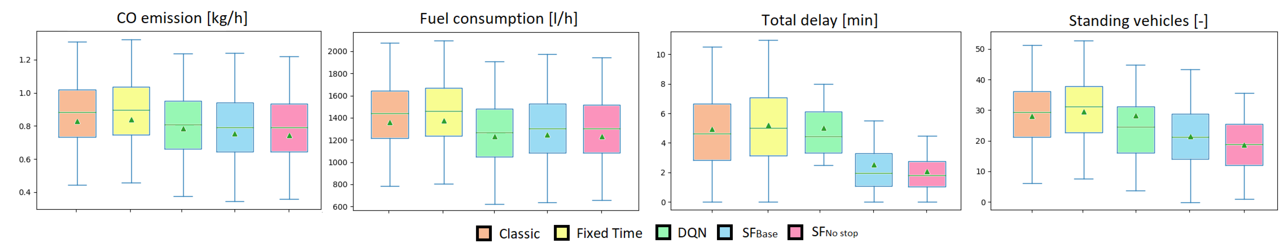
First, we look at a uniform flow distribution and compare the rule-based and learning algorithms by using boxplots in Figure 1. Each agent is given 1000 random episodes, and their performance is compared with the metrics of CO, fuel consumption, total delay, and standing vehicles. Each boxplot represents the average values based on 1000 random episodes that are identical. With the help of the boxplots, we can see the mean (green triangle) and the median (green line) of the data. Meanwhile, the boxes show points between the lower and upper quartiles (Q1–Q3), and the whiskers on top of the boxes are for the minimum and maximum ranges. The lower the values and the smaller the boxes are, the better.

In Figure 1, values are as expected; the fixed time agent scores the worst in each metric, followed by the classic agent. Although classic optimizes for the delay, the DQN and SF techniques perform better, as was shown before in the literature. The difference between $S{F}_{base}$ and DQN is marginal in CO and fuel usage, while the $SFbase$ agent did not explicitly learn to optimize the objective generated by ${\mathbf{w}}_{\mathbf{eval}}=[1,1,1,1,1]$. A more apparent advantage is observable when comparing the total delays of an episode. Both $SF$ agents reduce the average delay minutes of the network. Note: $S{F}_{no\_stop}$ tries to optimize the number of vehicles halting in the scene. Interestingly, despite the different perspectives, it performs almost as well as $S{F}_{base}$. The reason lies in our method. Each policy has its SF prediction, and when combined with ${\mathbf{w}}_{\mathbf{eval}}$, each has an idea of the best action. Furthermore, ${\pi }_4$ knows how to minimize the halting, but in situations when the scene is optimal for ${\pi }_4$, the others can contribute to the decision, as Equation (5) suggests. This performs similarly to the all-optimizing $S{F}_{base}$. In regard to performing better than DQN, we can state that the complex reward function of five components allows the agent to optimize for the one with the highest magnitude: fuel consumption.

Table 2. Comparison of the performance between the different solutions in case of uniform flows.

Agent	${\mathit{t}}_{\mathbf{prio}}$		CO Emission		Fuel Consumption		Standing Vehicles		Total Delay
	%	min	%	kg/h	%	l/h	%	-	%	min
Fixed Time	100	0.51	100	0.84	100	1339.2	100	29.8	100	5.19
Classic	81.3	0.41	97.6	0.82	99.8	1336.8	94.7	28.2	94.8	4.92
DQN	63.8	0.32	94.0	0.79	90.7	1214.7	95.9	28.6	95.3	4.95
$S{F}_{base}$	24.7	0.12	89.2	0.75	92.3	1236.0	73.0	21.7	48.7	2.53
$S{F}_{nostop}$	26.9	0.13	88.1	0.74	91.5	1225.6	70.2	20.9	39.7	2.06

indicates the mean values of Figure 1 and displays the percentage of the improvement compared to the fixed time baseline. We can observe that DQN has the best score in fuel consumption as anticipated, but is closely followed by the $SF$ agents. Meanwhile, the other metrics show a more significant difference in favor of our method. Table 2 also highlights the PV total waiting time average among the 1000 episodes, and it is clear that the $SF$ methods allow the PV to pass approximately four times faster on average.

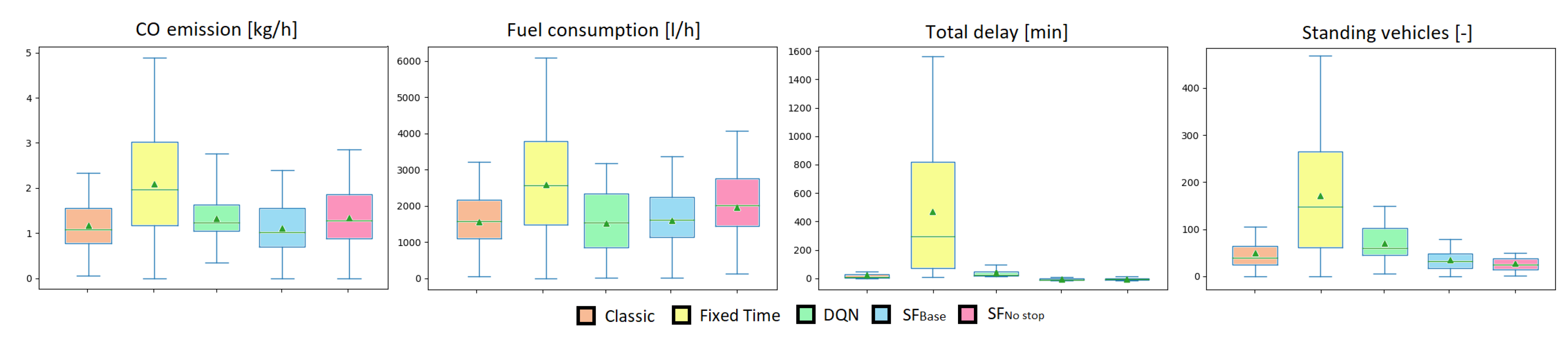
As an ablation of the possibilities using SF-based agents, we investigated 1000 scenarios using asymmetric flows. This meant that either the EW or the NS lanes had drastically more incoming vehicles. As seen in Figure 2, the metrics of the fixed time agent suffered the most. This can be also seen in

Table 3. Comparison of the performance between the different solutions in case of asymmetric flows.

Agent	${\mathit{t}}_{\mathbf{prio}}$		CO Emission		Fuel Consumption		Standing Vehicles		Total Delay
	%	min	%	kg/h	%	l/h	%	-	%	min
Fixed Time	100	150.1	100	2.1	100	2595.1	100	173.6	100	460.3
Classic	0.4	0.69	53.3	1.12	60.1	1561.7	28.8	49.9	4.9	22.4
DQN	1.2	1.8	57.6	1.21	59.8	1554.4	46.1	80.0	12.5	57.7
$S{F}_{base}$	0.1	0.18	52.8	1.11	61.5	1597.8	20.6	35.7	2.2	10.3
$S{F}_{nostop}$	0.1	0.23	63,8	1.34	75.6	1963.7	23.9	41.5	1.9	9.1

. It is natural that switching between the methods equally in an uneven load results in the worst performance. Our attention is guided toward our learning methods. DQN falters the most in standing vehicles because, as mentioned before, it learns to optimize primarily for fuel consumption. $S{F}_{base}$ could perform the best in all metrics except fuel. Visibly, $S{F}_{no\_stop}$ could achieve the most negligible variance and mean regarding standing vehicles, but all other metrics were affected. Due to the long queues trying to pass the intersections, $t_{prio}$ increased for all agents, but $S{F}_{base}$ could keep it small. In reality, as the prioritized vehicle entered the scene, it opened the route and allowed all preceding cars to pass. This caused some degradation in other metrics, but it seems reasonable and acceptable.

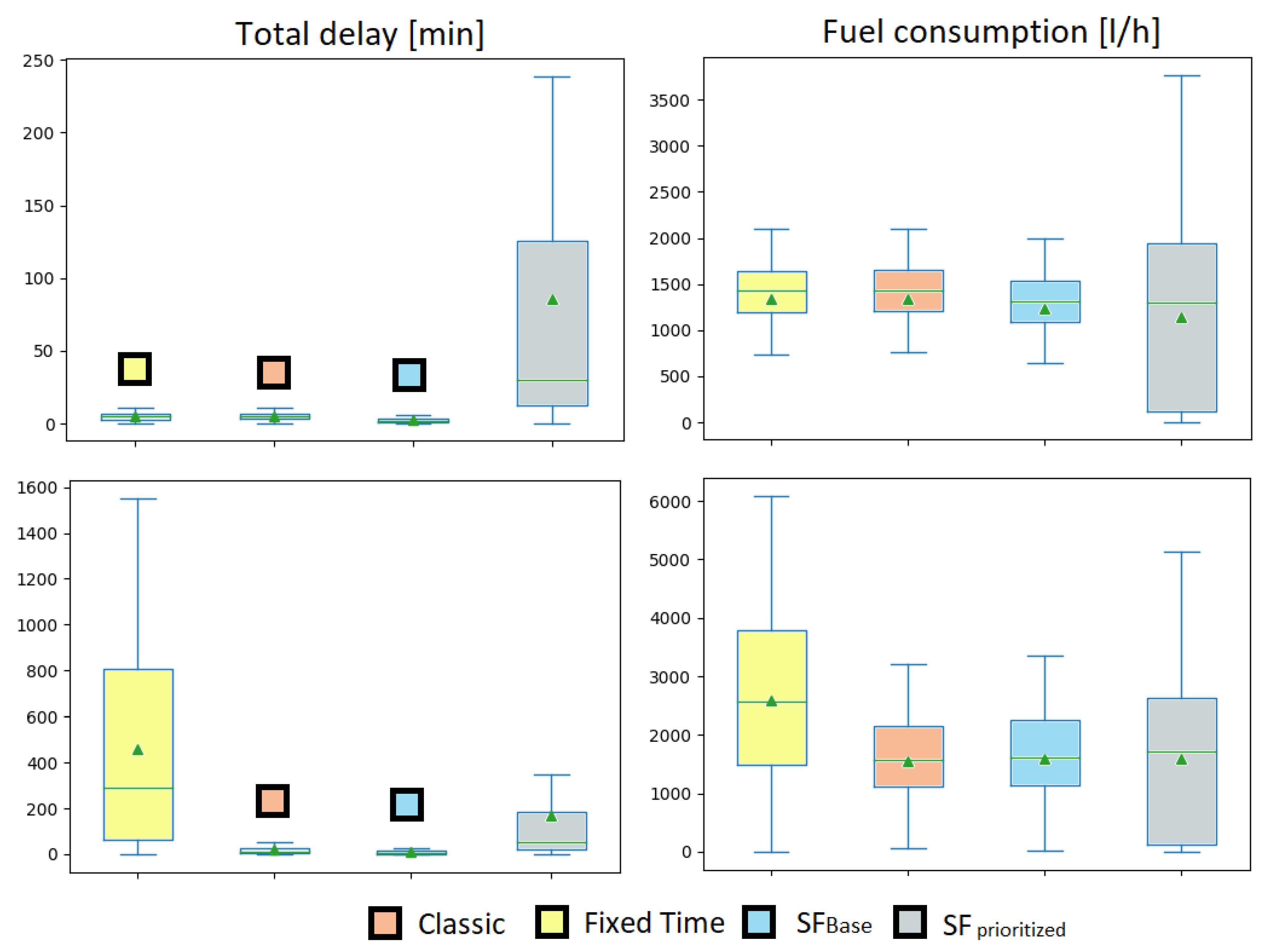
Lastly, Figure 3 shows how selected metrics change when evaluating the only prioritized interested policy ${\pi }_5$. The total delay and fuel consumption worsening is significant in both the uniform and asymmetric cases, but $S{F}_{prioritized}$ managed to achieve $t_{prio}=0$. In the case of uneven loads, the $S{F}_{prioritized}$ outperformed the baseline. This indicates that with our adaptive preferences, we could allow the prioritized vehicles to move when needed and optimize the network emissions altogether otherwise. By using SF values to estimate the Q values, we gained a method to set the traffic preferences on the fly adaptively. We can change the ${\mathbf{w}}_{\mathbf{eval}}$ any time and have a more suitable local solution for the intersection. Additionally, our method needs no supplementary sensors, as we have loop detectors. The PV’s location measurement can be based on GPS and internet communication with the traffic control system.

6. Conclusions

In summary, our work emphasizes the adaptivity of our method, which uses SFs for TSC optimization. By introducing reward components or features, we can design multi-objective RL that can be used to train agents for various target tasks.

To the best of our knowledge, we are the first to use SFs in TSC optimization and have successfully demonstrated their advantages over other baselines. Our approach allows for the alteration of a trained agent’s behavior within the range of the SF combinations simply by adjusting the weight vector $\mathbf{w}$. This means that we can prioritize different objectives, such as queue length or total CO emissions, without a significant performance deterioration.

We have thoroughly tested our method in different scenarios and shown that it outperforms known algorithms for optimizing a single four-way intersection. Additionally, our approach remains capable of adapting to new and personalized preferences without requiring the agent to be retrained. Furthermore, we demonstrate that prioritized vehicles could be given the freeway when necessary, thus helping services such as public transport or emergency vehicles.

Moving forward, we plan to extend our method to complex networks and multiple intersections with cooperation between them. An exciting direction for future research is investigating the objective preferences of individual networks, which poses significant challenges but also has high potential. Furthermore, we aim to broaden our method and explore how a general optimizing network could recognize different scenarios and select preferences based on them.

Overall, our work provides yet another powerful ML-based method for optimizing traffic at intersections, with promising applications for real-world traffic management systems.