Low Complexity Speech Enhancement Network Based on Frame-Level Swin Transformer

Abstract

In recent years, Transformer has shown great performance in speech enhancement by applying multi-head self-attention to capture long-term dependencies effectively. However, the computation of Transformer is quadratic with the input speech spectrograms, which makes it computationally expensive for practical use. In this paper, we propose a low complexity hierarchical frame-level Swin Transformer network (FLSTN) for speech enhancement. FLSTN takes several consecutive frames as a local window and restricts self-attention within it, reducing the complexity to linear with spectrogram size. A shifted window mechanism enhances information exchange between adjacent windows, so that window-based local attention becomes disguised global attention. The hierarchical structure allows FLSTN to learn speech features at different scales. Moreover, we designed the band merging layer and the band expanding layer for decreasing and increasing the spatial resolution of feature maps, respectively. We tested FLSTN on both 16 kHz wide-band speech and 48 kHz full-band speech. Experimental results demonstrate that FLSTN can handle speech with different bandwidths well. With very few multiply–accumulate operations (MACs), FLSTN not only has a significant advantage in computational complexity but also achieves comparable objective speech quality metrics with current state-of-the-art (SOTA) models.

1. Introduction

Speech enhancement (SE) is a technology for recovering clean speech signals from noisy backgrounds [1], which covers a wide range of applications, including voice calls, teleconferencing, hearing aid devices, etc. [2]. Although SE technology appears to be a simple process of speech recovery, the algorithms involved are extensive and diverse. Traditional SE approaches such as spectral subtraction [3] and Wiener filtering [4] can effectively deal with stationary noise but are powerless to suppress the non-stationary noise that is widely present in the natural environment. In recent years, with the introduction of deep learning, SE technology based on deep learning has attracted extensive attention [5,6]. The method based on deep learning has strong modelling ability for nonlinear complex signals, which can effectively make up for the shortcomings of traditional methods, and has become the current mainstream.

Convolutional neural networks (CNNs) have a relatively large advantage in extracting local features but have limitations in modelling a wider range of dependencies for low-level features [7]. Traditional models which use CNN block as their backbone network cannot learn global and long-term information well. But the information is necessary and important for many SE tasks. Encouraged by the success of Transformer [8] in the field of natural language processing (NLP), speech enhancement Transformer (SETransformer) [9] applied Transformer to speech enhancement tasks for the first time. And with the deepening of research, advanced Transformer-based models such as two-stage transformer neural network (TSTNN) [10] and Uformer (Unet based dilated complex & real dual-path conformer) [11] have been gradually developed. However, Transformer has a limitation that the high computational complexity makes it difficult to implement on some devices with limited computing power. Recently, researchers developed a hierarchical Swin Transformer architecture in [12], which takes the Swin Transformer as the visual backbone and achieves SOTA performance in semantic segmentation, object detection, and image classification. In the audio field, Chen [13] first employed Swin Transformer for audio classification and achieved SOTA results on several audio datasets. This implies that Swin Transformer also has high research value in the field of audio processing.

In order to explore the application potential of Swin Transformer in speech enhancement tasks, we propose a novel frame-level Swin Transformer architecture for speech enhancement. Specifically, the frame-level Swin Transformer takes several consecutive frames as a local window and restricts self-attention within it to make the complexity becomes linear to spectrogram size. A shifted window mechanism is adopted to strengthen the information exchange between adjacent windows. The authors of [13] continued the processing method used in the image field by employing square windows to construct local windows. However, the time frequency features of speech are usually rectangular in shape, so the operation of padding a large number of zeros at the boundaries increases the amount of invalid computation. Our proposed frame-level Swin Transformer can adapt to different sizes of feature maps and directly process rectangular time frequency windows, so it is more computationally efficient. These ingenious designs not only consider the global modelling ability of Transformer, but also greatly reduce the computational cost of self-attention. We use frame-level Swin Transformer modules as the backbone of the proposed model FLSTN. Furthermore, the band merge layer and the band expand layer are designed for the reduction and restoration of the spatial resolution of the feature maps, respectively. The multi-scale and long-term speech feature information extracted by FLSTN is beneficial for the recovery of target speech in strong noise environments [14]. Experimental results show that FLSTN achieves the best performance while maintaining low complexity compared to other SOTA models.

The main contributions of this paper can be summarized as the following three points:

• Our study is the first work to explore the application of Swin Transformer structure in speech enhancement tasks.
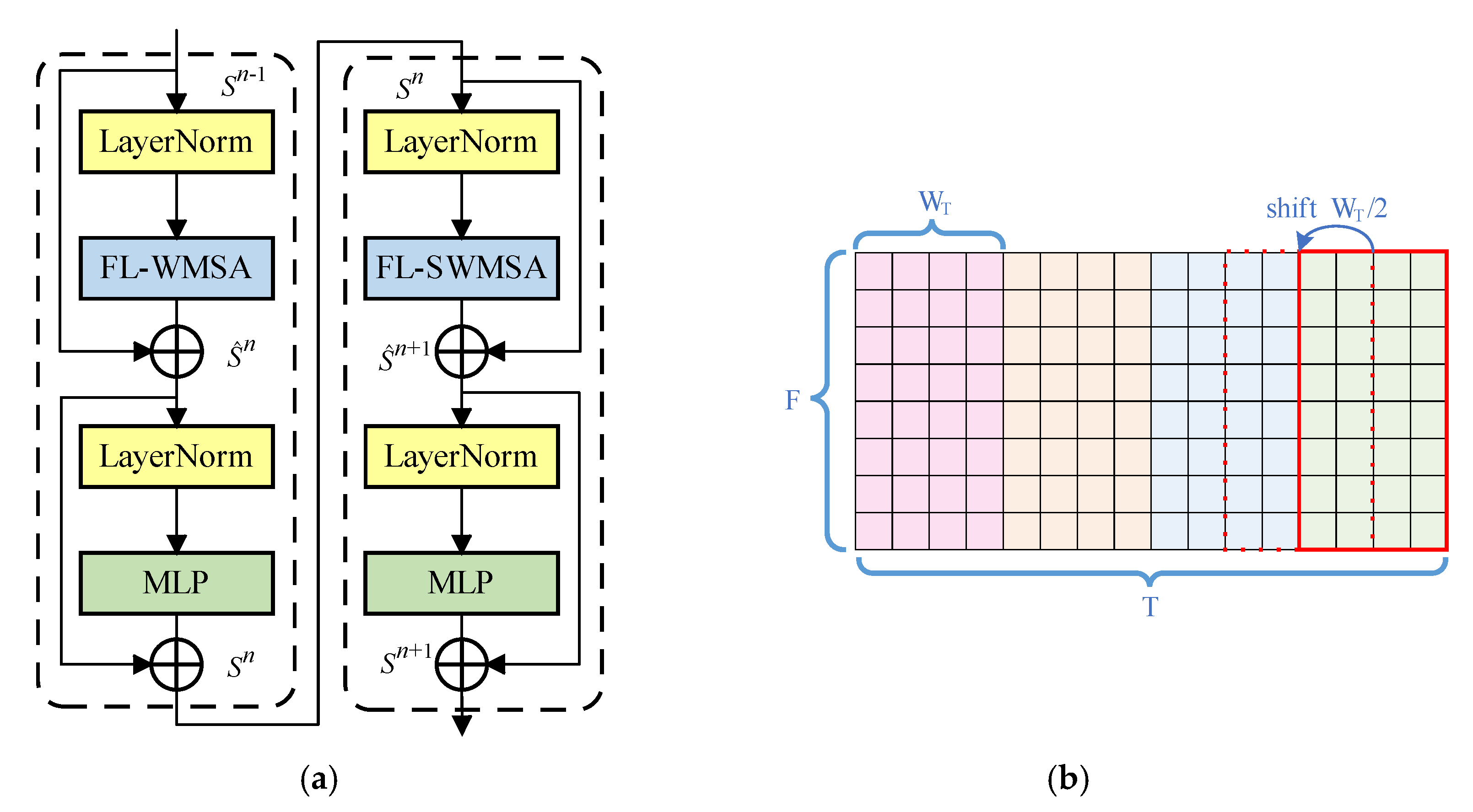
• We propose a novel frame-level Swin Transformer structure suitable for speech processing tasks, which adopts the frame-level shifted window mechanism for attention calculation. The proposed structure greatly saves computing resources, facilitates the construction of speech stream processing, and provides a new solution for future speech enhancement systems.
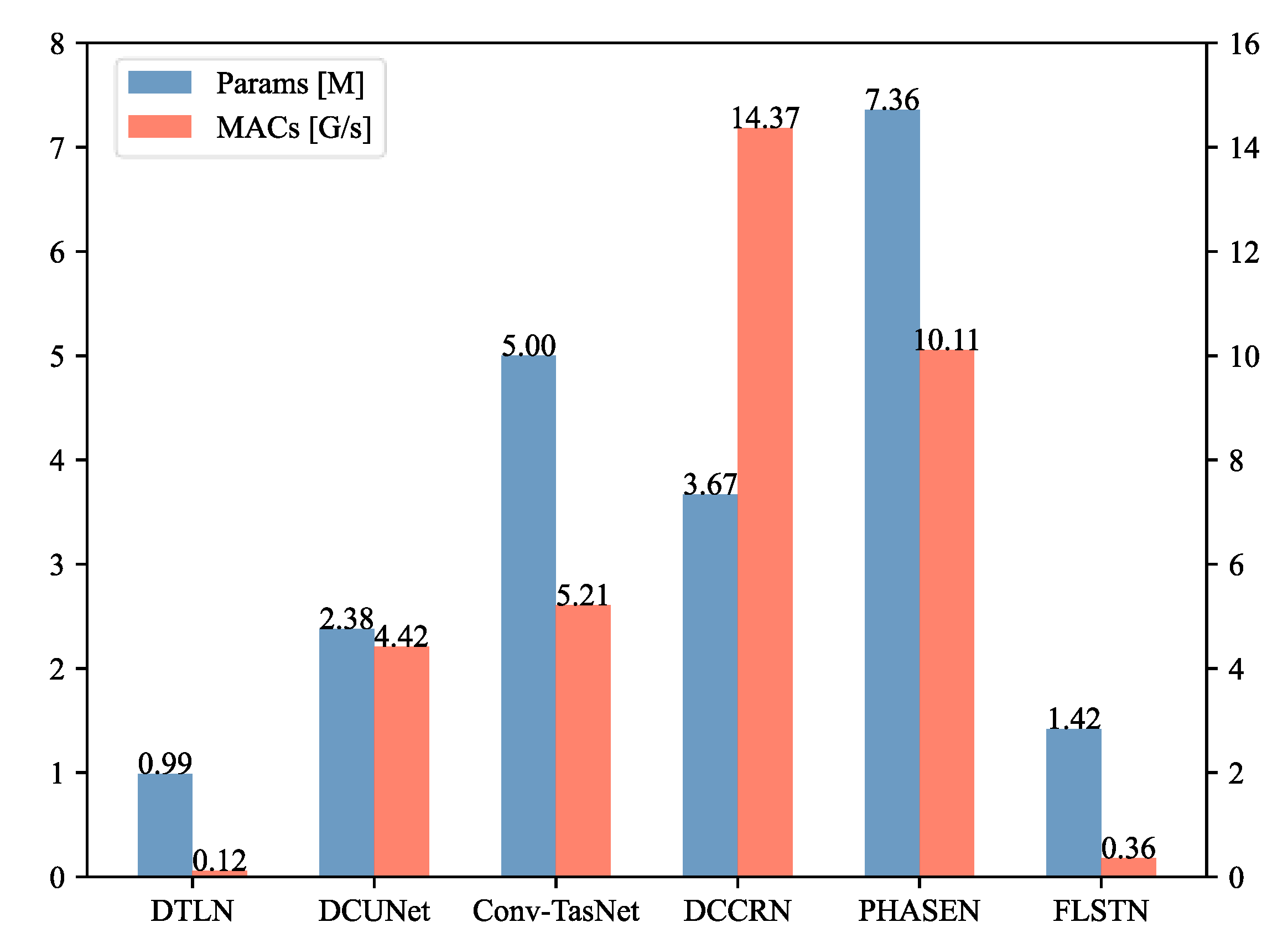
• The proposed FLSTN model utilizes frame-level Swin Transformer modules as the backbone, maintaining low computational complexity and achieving outstanding performance.

2. Related Work

2.1. CNN-Based Speech Enhancement Methods

Early speech enhancement methods were mainly based on traditional signal processing algorithms. With the development of deep CNN, many excellent CNN-based speech enhancement models have emerged, such as temporal convolutional neural network (TCNN) [15], deep complex U-Net (DCUNet) [16] and deep complex convolution recurrent network (DCCRN) [14]. Although CNN and its variants remain the main backbone architecture for speech enhancement tasks, the Transformer architecture with more powerful modelling capabilities has shown great potential. Our work is to explore a more suitable Transformer architecture for speech enhancement.

2.2. Transformer-Based Speech Enhancement Methods

Transformer was first proposed by [8] to solve machine translation problems. Not only limited to the field of NLP, current Transformer-based approaches have achieved SOTA performance in almost all fields. But Transformer also has its drawbacks. Taking speech enhancement as an example, most methods based on Transformer are complex, slow, and require high hardware requirements, which make them difficult to train. Therefore, it is imperative to find a variant Transformer structure that is more suitable for speech enhancement tasks. In our work, we try to utilize the Swin Transformer from image field as a new backbone for speech enhancement model.

3. Problem Formulation

Let us take a speech signal contaminated by independent additive noise as an example. Given a clean speech signal s(t) and a background noise signal c(t). The mixed noisy speech signal can be expressed by the following equation:

$$y(t)=s(t)+c(t)$$

(1)

Assume the speech is quasi-smooth [17], so it can be analyzed frame-by-frame using short-time Fourier transform (STFT). The STFT of the noisy speech is given by Equation (2).

$$Y(n,k)={\displaystyle \sum _{m=-\infty }^{\infty }y(m)w(n-m){{\displaystyle e}}^{-j2\pi km/L}}$$

(2)

Here w(n) denotes an analysis window function. k is the index of the discrete acoustic frequency, and the range is {1, 2, …, L}. L is the length of frequency analysis. n is the index of time-frame, and the range is {1, 2, …, N}. So, after STFT, we can represent the noisy speech signal as:

$$Y(n,k)=S(n,k)+C(n,k)$$

(3)

We take Y(n, k) as the input feature of the model and output the real mask M_r(n, k) and imaginary mask M_i(n, k). Complex ratio mask (CRM) [18] is employed to obtain the plural form of estimated speech. Inverse short-time Fourier transform (ISTFT) is responsible for converting $\widehat{S}(n,k)$ to a time domain signal $\widehat{s}(t)$.

$$\left\{\begin{array}{l}{\widehat{S}}_r=M_r{Y}_r-M_i{Y}_i\\ {\widehat{S}}_i=M_r{Y}_i+M_i{Y}_r\end{array}\right.$$

(4)

Signal approximation (SA) minimizes the difference between the estimated and clean speech by applying a loss function $L=Loss[\widehat{s}(t),s(t)]$, which usually gives better enhancement than direct estimation.

4. Method

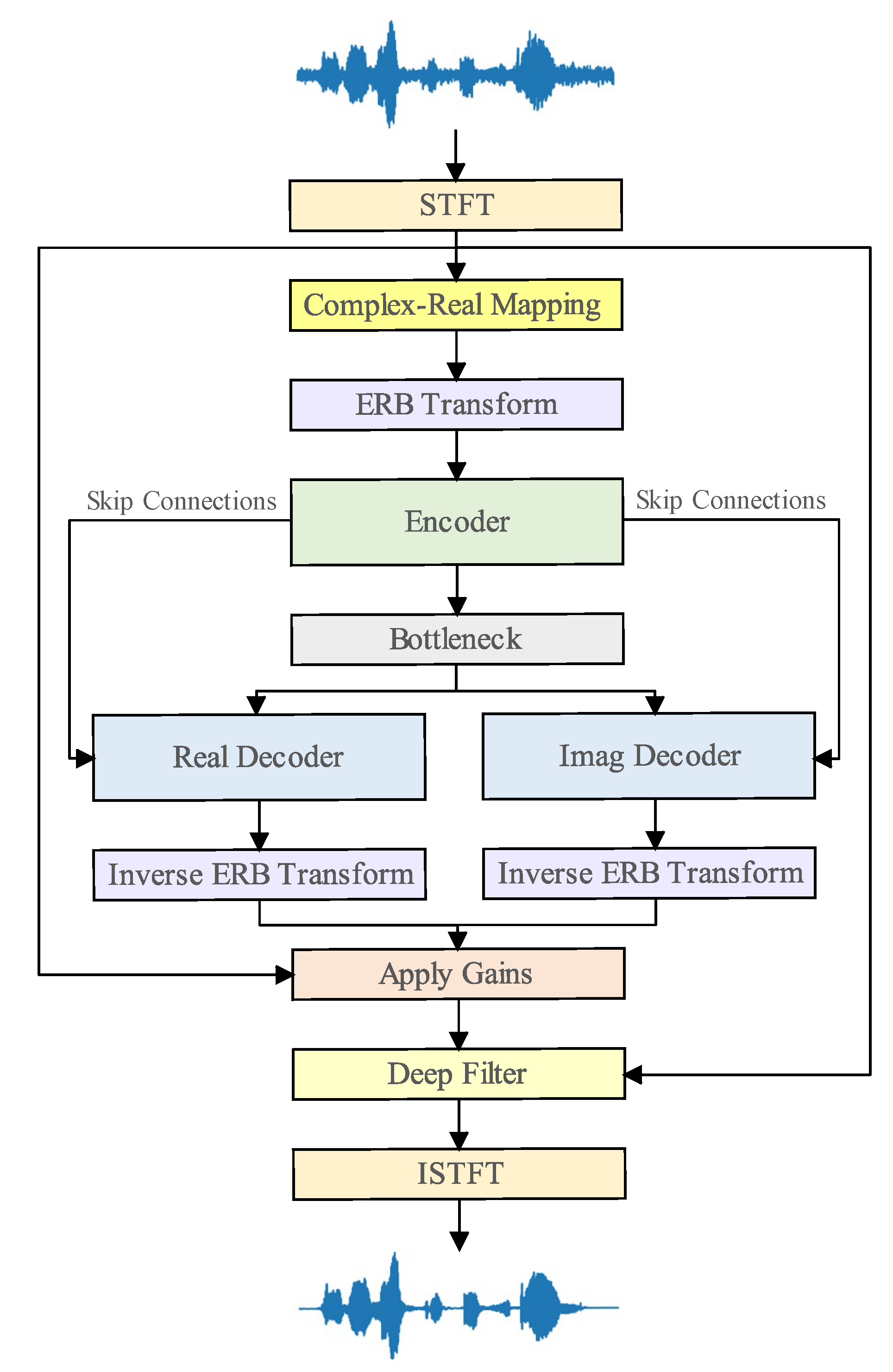
4.1. Architecture Overview

The overall architecture of FLSTN is illustrated in Figure 1. Firstly, complex spectral features are extracted from the noisy speech by STFT, and then mapped to a real number field by a complex-real mapping module. Equivalent rectangular bandwidth (ERB) scale is adopted to reduce the frequency dimension to 32 bands, which greatly reduces redundant calculation in high frequency bands. Figure 2a–c show the structures of encoder, bottleneck layer and decoder, respectively. The encoder responsible for down-sampling is composed of hierarchical frame-level Swin Transformer layers and band merging layers. The bottleneck layer is stacked by lightweight temporal-frequential convolution modules (TFCM) to enhance the long-term information learning ability of FLSTN. We also design a real decoder and an imaginary decoder symmetric to the encoder for up-sampling, which consist of frame-level Swin Transformer blocks and band expanding layers. Multi-scale low-level features and high-level features are fused by add-skip connections, thus retaining more abundant speech details. A deep filter [19] is employed to eliminate residual noise, especially nonlinear noise. Each module is elaborated in the following.

4.2. Complex-Real Mapping Module

Although the performance of complex networks is slightly better than real networks, their complexity is usually much higher. Therefore, in order to balance complexity and performance, we design a module that maps the complex features of speech to real features. The complex-real mapping module consists of a complex convolution layer, a complex-to-real projection layer, and a feature compression layer. In our experiment, the compression factor is set to 0.5.

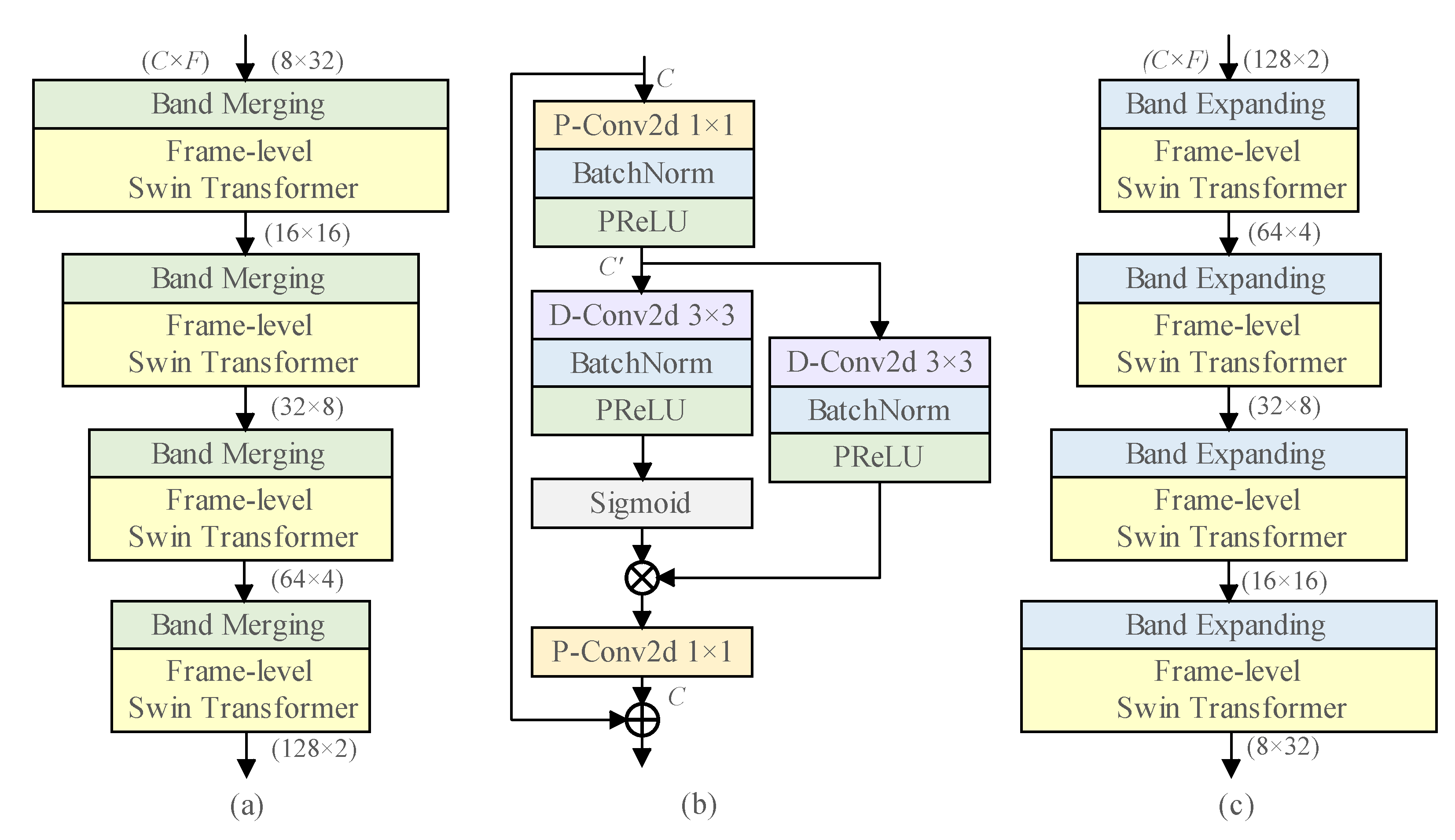
4.3. Frame-Level Swin Transformer

As shown in Figure 3a, a frame-level Swin Transformer layer is composed of two successive frame-level Swin Transformer blocks. Each Swin Transformer block [12] contains two layer normalization layers and a two-layer multi-layer perceptron (MLP) with Gaussian Error Linear Unit (GELU) activation function. The difference from traditional Transformer is that the multi-head self-attention (MSA) is replaced by frame-level window-based MSA (FL-WMSA) or frame-level shifted window-based MSA (FL-SWMSA). FL-WMSA restricts attention to each window, resulting in a lack of information interaction between windows, which makes FL-WMSA ineffective when used alone. Therefore, FL-SWMSA adds shifted window mechanism based on FL-WMSA to compensate for this deficiency. For FL-WMSA, we first split the feature map into N non-overlapping (F × W_T) windows, as shown in Figure 3b. Then we compute the self-attention limited to each window instead of the global self-attention calculation, so we can obtain N window self-attention matrices. In this study, W_T = 4. For FL-SWMSA, the window shifts towards past time by W_T/2 in length each time. It can be clearly found that frame-level Swin Transformer removes the square window limitation of the original Swin Transformer, which greatly enhances its universality. By analogy with [12], the complexity of traditional MSA and FL-WMSA can be described as follows.

$$\left\{\begin{array}{l}\mathrm{\Omega }(MSA)=4FT{C}^2+2{(FT)}^{2}C\\ \mathrm{\Omega }(FL-WMSA)=4FT{C}^2+2F^{2}T{W}_{T}C\end{array}\right.$$

(5)

where F, T and C denote the number of frequency bands, frames, and the channel dimension, respectively. For the complexity of the above two, FL-WMSA reduces the dominant second term by T/W_T times. The complexity of MSA is quadratic to T, while FL-WMSA is linear, and W_T is much small than T. As a result, the complexity of FL-WMSA is far less than that of MSA, which cannot be ignored in practical applications.

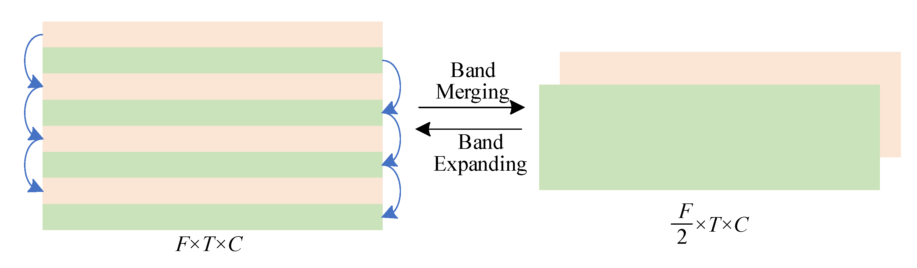
4.4. Band Merging and Expanding

Band merging and expanding layers reduce and restore the resolution of speech feature maps, respectively. For example, the band merging layer transforms a feature of shape (C × F × T) into $(2C\times \frac{F}{2}\times T)$, while the band expanding layer is responsible for restoring the feature size. Then the feature map is fed into frame-level Swin Transformer modules for deep representation learning. Notably, the band merging and expanding layers require almost no additional parameters, which further reduces the complexity of FLSTN. The graphical illustration of band merging and expanding is illustrated in Figure 4.

4.5. Lightweight TFCM

Long short-term memory (LSTM) can effectively model time series, but it requires many parameters, so we design a lightweight temporal-frequential convolution module as the basic unit of bottleneck layer instead of LSTM. The structure of the proposed lightweight TFCM is shown in Figure 2b. Firstly, the input channel C is compressed to C′ by a 1 × 1 2D pointwise convolution (P-Conv2d). Then we use a two-branch 2D dilated convolution (D-Conv2d) instead of D-Conv1d for multi-scale modeling along time dimension with a kernel size of 3 × 3. The output of one branch is restricted to (0, 1) by a sigmoid function and multiplied by the output of the other branch. In this experiment, we use 3 stacked lightweight TFCM blocks to form the bottleneck layer and each TFCM block consists of 6 TFCMs. The dilation rates of the two branches are 2ⁱ, 2^L−i, where L = 6 and I $\in$ {0, 1, 2, 3, 4, 5}. Complementary dilation rates enable the two branches to learn long-term and short-term dependencies simultaneously.

4.6. Apply Gains

The pre-estimated speech is generated by CRM, and it should be noted that we convert the mask to polar coordinates. The Cartesian coordinate representation of mask can also be expressed in polar coordinates:

$$\left\{\begin{array}{l}{M}_{mag}=\sqrt{M_r^2+M_i^2}\\ M_{pha}=\arctan 2(M_i,M_r)\end{array}\right.$$

(6)

The pre-estimated clean speech S_p can be calculated as below:

$$S_p=Y_{mag}•M_{mag}•{\exp }^{Y_{pha}+M_{pha}}$$

(7)

where Y_mag and Y_pha represent the magnitude and phase of noisy speech, respectively.

4.7. Deep Filter

We believe that the dot product operation of the mask-based method is inherently more inclined to remove linear noise, so we introduce a deep filter module to remove residual nonlinear noise. In deep filter module, each TF bin of the output spectrogram is mapped from adjacent local TF bins of the pre-estimated spectrogram. A deep filter is defined as follows:

$$S(t,f)={\displaystyle \sum _{i=0}^{N}D(i,t,f)•Y(t-i,f)}$$

(8)

$$S_{out}(t,f)=\theta •{S^{\prime }}_{out}(t,f)+(1-\theta )•S_p(t,f)$$

(9)

where D is the complex coefficients of the N^th order filter of the input spectrogram Y, and $\theta$ is the weighting factor. Previous studies [19,20] have shown that a deep filter can effectively enhance the harmonics of speech.

4.8. Loss Function

Both objective and subjective results reveal that better speech enhancement performance can be achieved *-96+when using suitable power compress loss. The spectrogram after power compression can be expressed as $S^p={\left|S\right|}^{\alpha }{e}^{i\theta }$, Thus, the real and imaginary parts can be formulated by

$$\left\{\begin{array}{l}{S}_r^p={\left|S\right|}^{\alpha }\cos \theta \\ S_i^p={\left|S\right|}^{\alpha }\sin \theta \end{array}\right.$$

(10)

The loss function $L_{RI}(\widehat{S},S)$, used to describe the similarity of the estimated complex spectrogram and the clean complex spectrogram can be given as

$$L_{RI}(\widehat{S},S)={‖{\widehat{S}}_r^p-S_r^p‖}_F^2+{‖{\widehat{S}}_i^p-S_i^p‖}_F^2$$

(11)

where $\widehat{S}$, ${\widehat{S}}_r^p$ and ${\widehat{S}}_i^p$ denote the estimated spectrogram, compressed estimated real part and compressed estimated imaginary part, respectively. $‖•{‖}_F$ is the Frobenius norm. Because magnitude is much more important than phase in speech enhancement tasks, we add compressed magnitude loss.

$$L_{mag}(\widehat{S},S)={‖|\widehat{S}{|}^{\alpha }-|S{|}^{\alpha }‖}_F^2$$

(12)

Total loss can be given by the following equation, where $\alpha =\frac{1}{3}$ in this paper.

$$Loss=L_{RI}(\widehat{S},S)+L_{mag}(\widehat{S},S)$$

(13)

5. Experiment

5.1. Experiment I

5.1.1. Dataset and Evaluation Metric

We first evaluate the enhancement effect of FLSTN on wideband speech at 16 kHz. All clean utterances come from the training set si_tr_s of Wall Street Journal (WSJ0) corpus [21], which consists of 9321 utterances from 101 speakers. We randomly select six speakers (three male and three female) for the validation set, and the clean speech for evaluation set is selected in the same way. The remaining samples from 89 speakers are used for training. The noises of training and validation sets are from Interspeech 2021 deep noise suppression (DNS) noise set [22], and each clean utterance is corrupted with three types of noises randomly selected from 65303 noises at signal-to-noise ratios (SNRs) between −5 dB and 15 dB with an interval of 1 dB. In order to evaluate the model performance under various unknown noises, we use the babble and factory1 noises from NOISEX92 [23] for evaluation set. The SNR levels are {0 dB, 5 dB, 10 dB}.

We select perceptual evaluation of speech quality (PESQ) [24], short-time objective intelligibility (STOI) [25] and composite metrics CSIG, CBAK, COVL [26] as evaluation metrics. The typical values for PESQ range from −0.5 to 4.5 and STOI values range from 0 to 1. Three other composite metrics: CSIG for signal distortion MOS (Mean Opinion Score), CBAK for background noise interferences, and MOS and COVL for overall speech quality MOS. All MOSs range between 1 and 5, i.e., 1-bad, 2-poor, 3-fair, 4-good, 5-excellent.

5.1.2. Experimental Setup and Baselines

In our experiments, the window length and hop size of STFT are 25 ms and 12.5 ms, and the FFT length is 400. We use the Adam optimizer with an initial learning rate of 0.001 as the optimizer. A dynamic strategy is used in the training stage. More specifically, the learning rate is halved when the loss of validation set does not improve for 3 consecutive epochs. The model is selected by early stopping. If there is no loss improvement for 10 consecutive epochs, the training stage will stop and the best performing model will be taken. All models are trained for a maximum of 100 epochs to avoid over-adaptation.

DTLN: a real-time noise suppression method based on stacked double signal transformation LSTM network [27]. It has less than 1 M parameters.

DCUNet: a variant UNet based on the complex domain [16]. We use DCUNet-16 for comparison, and the channels in the encoder are set to {32, 32, 64, 64, 64, 64, 64, 64}.

Conv-TasNet: a deep learning framework for end-to-end full convolutional time-domain speech separation [28]. We set the number of speakers to one and apply the framework to speech enhancement tasks.

DCCRN: a deep complex convolutional recurrent network [14]. It ranks first on the real-time track for the Interspeech 2020 DNS challenge. We use DCCRN-CL for comparison, and the channels in the encoder are set to {32, 64, 128, 256, 256, 256}.

PHASEN: a phase-and-harmonics-aware speech enhancement network [29]. It is a two-stream network composed of an amplitude stream and a phase stream for simultaneously predicting amplitude and phase.

5.1.3. Experimental Results

We use the utterances polluted by babble and factory1 noises as the evaluation set to test the generalization of the model under different SNRs. The results are shown in

Table 1. Experimental results on WSJ0-babble and WSJ0-factory1 evaluation sets.

Model	SNR	Babble					Factory1
		PESQ	STOI	CSIG	CBAK	COVL	PESQ	STOI	CSIG	CBAK	COVL
Noisy	0 dB	1.09	0.684	2.30	1.40	1.58	1.06	0.683	2.22	1.43	1.54
DTLN		1.29	0.780	2.65	1.94	1.89	1.34	0.805	2.61	2.06	1.92
DCUNet		1.31	0.794	2.54	2.02	1.84	1.36	0.820	2.59	2.14	1.91
Conv-TasNet		1.32	0.838	2.85	2.12	2.03	1.32	0.837	2.78	2.15	2.01
DCCRN		1.35	0.828	2.52	1.65	1.86	1.33	0.836	2.44	1.72	1.83
PHASEN		1.33	0.810	2.67	1.60	1.92	1.43	0.830	2.76	1.74	2.04
FLSTN(Pro.)		1.45 *	0.825	3.04	2.20	2.19	1.54	0.843	3.09	2.33	2.27
Noisy	5 dB	1.18	0.799	2.68	1.73	1.85	1.13	0.803	2.58	1.74	1.79
DTLN		1.63	0.886	3.19	2.32	2.36	1.62	0.889	3.04	2.37	2.30
DCUNet		1.68	0.895	3.11	2.47	2.34	1.70	0.903	3.03	2.53	2.32
Conv-TasNet		1.68	0.915	3.34	2.49	2.48	1.64	0.912	3.21	2.49	2.40
DCCRN		1.79	0.916	3.14	1.94	2.43	1.70	0.917	2.95	1.94	2.29
PHASEN		1.77	0.907	3.27	1.90	2.48	1.80	0.912	3.21	1.97	2.47
FLSTN(Pro.)		1.97	0.916	3.65	2.72	2.78	2.00	0.918	3.58	2.76	2.77
Noisy	10 dB	1.37	0.887	3.09	2.13	2.18	1.32	0.894	3.01	2.13	2.13
DTLN		2.10	0.939	3.71	2.70	2.88	2.01	0.938	3.49	2.68	2.73
DCUNet		2.19	0.946	3.69	2.96	2.92	2.18	0.948	3.54	2.98	2.84
Conv-TasNet		2.15	0.954	3.83	2.88	2.98	2.10	0.952	3.69	2.86	2.89
DCCRN		2.39	0.956	3.76	2.27	3.06	2.24	0.958	3.51	2.23	2.86
PHASEN		2.34	0.954	3.83	2.23	3.07	2.30	0.954	3.70	2.25	2.99
FLSTN(Pro.)		2.55	0.957	4.19	3.23	3.36	2.50	0.957	4.04	3.20	3.27
Noisy	AVG.	1.21	0.790	2.69	1.75	1.87	1.17	0.793	2.60	1.77	1.82
DTLN		1.67	0.868	3.18	2.32	2.38	1.66	0.878	3.05	2.37	2.31
DCUNet		1.73	0.878	3.11	2.48	2.37	1.75	0.891	3.05	2.55	2.36
Conv-TasNet		1.72	0.902	3.34	2.50	2.50	1.69	0.900	3.23	2.50	2.43
DCCRN		1.84	0.902	3.14	1.95	2.45	1.76	0.903	2.97	1.96	2.33
PHASEN		1.81	0.890	3.26	1.91	2.49	1.84	0.899	3.22	1.99	2.50
FLSTN(Pro.)		1.99	0.899	3.63	2.72	2.78	2.01	0.906	3.57	2.77	2.77

* In each case, the best result is highlighted by a boldface number.

. We can intuitively see that the results show consistency for the two different noises. FLSTN demonstrates excellent performance in terms of both PESQ, STOI and the three MOSs when compared with other SOTA models. For babble noise, compared with unprocessed noisy speech, PESQ improves by 0.78 on average, STOI improves by 10.9% on average, and the three MOSs improve by 0.94, 0.97, and 0.91, respectively. Similarly, for factory1 noise, PESQ and STOI are improved by 0.84 and 11.3%, and the three MOSs are improved by 0.97, 1.00 and 0.95, respectively. Among all the metrics, CSIG and CBAK show more improvement than others. This means that our method introduces less interference noise and recovers speech components effectively during the enhancement process. It also suppresses background noise strongly and improves the overall quality and listening effect of speech, making speech distortion and background noise hardly detectable. At low SNRs, the speech enhancement performance of all models under factory1 noise is lower than that under babble noise, which may be attributed to the effect of the spectral structure of different noise sources. Because babble noise is dominated by human voice, its spectral structure is very similar to that of clean speech. This increases the difficulty of distinguishing noise from clean speech, especially at low SNRs. In addition, the advantage of our method is not weakened compared with other methods at 0 dB, indicating that our model also has good performance at low SNR. Better speech quality indicates the effectiveness of the proposed frame-level Swin Transformer structure.

An illustrative diagram of the number of parameters and MACs for the proposed FLSTN and all competing baselines is shown in Figure 5. FLSTN requires only 1.42 M parameters and 0.36 G MACs per second, which provides a significant complexity advantage over other baselines except DTLN. Although the complexity of FLSTN is slightly higher than that of DTLN, we believe that it is well worthwhile to increase the computational effort by a small amount in exchange for a great improvement in performance.

5.2. Experiment II

5.2.1. Dataset and Evaluation Metric

In Experiment II, we use the VoiceBank-DEMAND dataset at 48 kHz. The clean speech in this dataset derives from the VoiceBank corpus [30], which consists of 28 speakers for training (11,572 utterances) and two additional speakers for evaluation (824 utterances), where male speakers and female speakers are equal in number. The noises of training set consist of 8 kinds of noises from DEMAND corpus [31] and two kinds of artificially generated noises (SNRs are 0 dB, 5 dB, 10 dB and 15 dB respectively). The evaluation set is generated by five kinds of unseen noises from DEMAND (SNRs are 2.5 dB, 7.5 dB, 12.5 dB and 17.5 dB respectively).

The evaluation metrics used in experiment II are the same as those in experiment I.

5.2.2. Experimental Setup and baselines

Due to lack of validation set for VoiceBank-DEMAND dataset, our network is trained on the training set for 50 epochs with a fixed learning rate of 0.0005. The STFT configuration and parameter settings are the same as in experiment I, except that the sampling rate and FFT length are changed to 48 kHz and 1200 respectively.

The baseline models for experiment II include RNNoise [32], NSNet2 [33], PercepNet [34], DCCRN [14], DCCRN+ [20], S-DCCRN [35], DeepFilterNet [36], and FullSubNet+ [37]. It should be noted that the data we use are provided by relevant papers, and the unreported values of related works are indicated as ‘-‘.

5.2.3. Experimental Results

We evaluate the applicability of FLSTN to the more challenging 48 kHz full-band speech in experiment II.

Table 2. Experimental results on VoiceBank-DEMAND test set.

Model	Year	Params[M]	MACs[G/s]	PESQ	STOI	CSIG	CBAK	COVL
Noisy	-	-	-	1.97	0.921	3.34	2.44	2.63
RNNoise	2018	0.06 *	0.04	2.33	0.922	3.40	2.51	2.84
PercepNet	2020	8.00	0.80	2.73	-	-	-	-
DCCRN	2020	3.70	14.36	2.54	0.938	3.74	3.13	2.75
NSNet2	2021	6.17	0.43	2.47	0.903	3.23	2.99	2.90
DCCRN+	2021	3.30	-	2.84	-	-	-	-
S-DCCRN	2022	2.34	-	2.84	0.940	4.03	2.97	3.43
DeepFilterNet	2022	1.78	0.35	2.81	0.942	4.14	3.31	3.46
FullSubNet+	2022	8.67	30.06	2.88	0.940	3.86	3.42	3.57
FLSTN	2022	1.42	0.38	2.88	0.944	4.18	3.43	3.53

* In each case, the best result is highlighted by a boldface number.

shows the comparison results between FLSTN and other SOTA methods. As can be found, FLSTN requires only a very few parameters and MACs to achieve the best scores for four metrics. The reason for this superior performance may be that FLSTN adopts Transformer as the backbone, which has stronger learning ability than other CNN-based models. It also uses a shifted window strategy to better capture the long-term features of the speech signal. These techniques enable FLSTN to produce clear and natural speech outputs with minimal distortion and noise. Although the COVL score of FLSTN is 0.04 lower than that of FullSubNet+, the complexity of the latter is obviously much higher. Incidentally, although RNNoise requires the fewest parameters and MACs, it significantly performs much worse than other methods. In conclusion, FLSTN can achieve satisfactory quality of enhanced speech while maintaining low complexity, which further emphasizes its excellent speech enhancement performance.

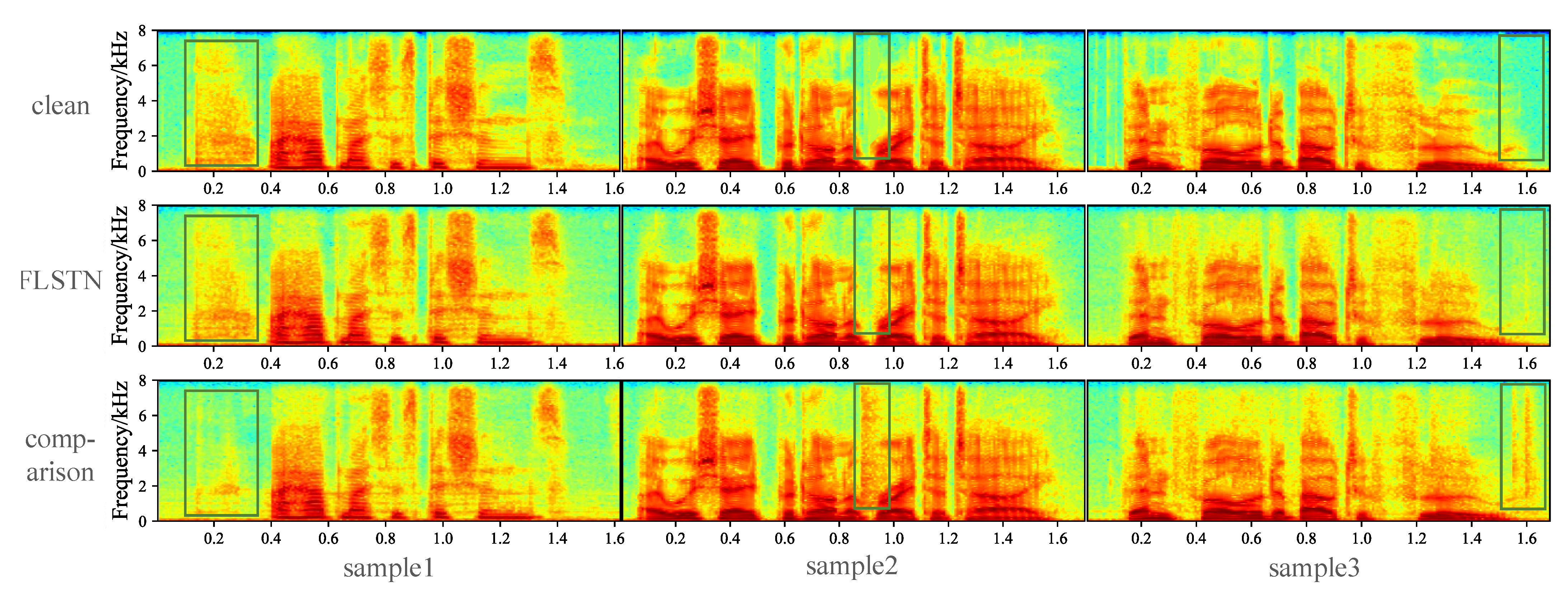
5.2.4. The Influence of Frame-Level Swin Transformer

To further demonstrate the effectiveness of our proposed frame-level Swin Transformer, we also designed an additional architecture with FLSTN for an ablation study. In this comparison model, we replace all frame-level Swin Transformer modules in the encoder and decoder of FLSTN with 2D convolution and transposed convolution with the same channel dimension, respectively. Each convolution or transpose convolution layer is followed by a 2D batch normalization layer and a parametric rectified linear unit (PReLU) activation function. The remaining configurations are identical to FLSTN. The results of the ablation study are shown in

Table 3. FLSTN vs. comparison model.

Model	PESQ	STOI	CSIG	CBAK	COVL
FLSTN	2.88 *	0.944	4.18	3.43	3.53
comparison	2.57	0.939	3.86	3.27	3.20

* In each case, the best result is highlighted by a boldface number.

and Figure 6.

It is obvious that FLSTN with frame-level Swin Transformer as the backbone outperforms the comparison model in all metrics. Furthermore, from Figure 6, we can find that the speech spectrograms enhanced by FLSTN are closer to the clean spectrograms. Compared with the comparison model, FLSTN has better denoising effect and loses less spectral information. We think there are three main reasons for the significant difference in scores between the two methods. First, Swin Transformer can capture long-distance dependencies in spectrograms, while CNN is limited by local receptive fields. Second, Swin Transformer can easily fuse multi-scale features, while CNN needs additional upsampling or downsampling operations. Third, Swin Transformer can adaptively adjust attention weights, while CNN needs to predefine kernel size and stride. Therefore, we believe that Swin Transformer is effective for speech enhancement because it can better extract details and structural information from speech signals and adapt to speech feature changes under different noise environments.

6. Conclusions

In this work, we proposed FLSTN, a low complexity speech enhancement network based on frame-level Swin Transformer. FLSTN has a lightweight structure and achieves SOTA results for both wideband and full-band speech enhancement tasks. The backbone of FLSTN is the frame-level Swin Transformer, which utilizes frame-level window attention to replace the global attention of spectrums, thus reducing the computational complexity of the network. We believe that the frame-level Swin Transformer has great potential for other speech processing tasks. Most notably, the frame-level shifted window mechanism can capture relevant and long-term historical information from adjacent windows, which is very suitable for building real-time speech streaming processing systems. In our future work, we will investigate different architectures and hyperparameters of the frame-level Swin Transformer to further enhance its robustness and performance for speech enhancement in noisy and reverberant environments. Moreover, we will apply our approach to other speech processing tasks, such as echo cancellation and speech recognition.

References

1. Loizou, P.C. Speech Enhancement: Theory and Practice; CRC Press: Boca Raton, FL, USA, 2007. [Google Scholar]
2. Kumar, S.; Kumar, B.; Kumar, N. Speech enhancement techniques: A review. Rungta Int. J. Electr. Electron. Eng. 2016, 1, 183–185. [Google Scholar]
3. Boll, S. Suppression of acoustic noise in speech using spectral subtraction. IEEE Trans. Acoust. Speech Signal Process. 1979, 27, 113–120. [Google Scholar] [CrossRef] [Green Version]
4. Scalart, P. Speech enhancement based on a priori signal to noise estimation. In Proceedings of the 1996 IEEE International Conference on Acoustics, Speech, and Signal Processing Conference, Atlanta, GA, USA, 9 May 1996; pp. 629–632. [Google Scholar]
5. Zhou, N.; Du, J.; Tu, Y.-H.; Gao, T.; Lee, C.-H. A speech enhancement neural network architecture with SNR-progressive multi-target learning for robust speech recognition. In Proceedings of the 2019 Asia-Pacific Signal and Information Processing Association Annual Summit and Conference (APSIPA ASC), Lanzhou, China, 1 June 2019; pp. 873–877. [Google Scholar]
6. Wu, B.; Yu, M.; Chen, L.; Xu, Y.; Weng, C.; Su, D.; Yu, D. Distortionless multi-channel target speech enhancement for overlapped speech recognition. arXiv 2020, arXiv:2007.01566. [Google Scholar]
7. O’Shea, K.; Nash, R. An introduction to convolutional neural networks. arXiv 2015, arXiv:1511.08458. [Google Scholar]
8. Vaswani, A.; Shazeer, N.; Parmar, N.; Uszkoreit, J.; Jones, L.; Gomez, A.N.; Kaiser, Ł.; Polosukhin, I. Attention is all you need. Adv. Neural Inf. Process. Syst. 2017, 30, 5998–6008. [Google Scholar]
9. Yu, W.; Zhou, J.; Wang, H.; Tao, L. SETransformer: Speech Enhancement Transformer. Cogn. Comput. 2022, 14, 1152–1158. [Google Scholar] [CrossRef]
10. Wang, K.; He, B.; Zhu, W.-P. TSTNN: Two-stage Transformer based neural network for speech enhancement in the time domain. In Proceedings of the 2021 IEEE International Conference on Acoustics, Speech and Signal Processing (ICASSP), Toronto, ON, Canada, 6–11 June 2021; pp. 7098–7102. [Google Scholar]
11. Fu, Y.; Liu, Y.; Li, J.; Luo, D.; Lv, S.; Jv, Y.; Xie, L. Uformer: A unet based dilated complex & real dual-path conformer network for simultaneous speech enhancement and dereverberation. In Proceedings of the 2022 IEEE International Conference on Acoustics, Speech and Signal Processing (ICASSP), Singapore, 22–27 May 2022; pp. 7417–7421. [Google Scholar]
12. Liu, Z.; Lin, Y.; Cao, Y.; Hu, H.; Wei, Y.; Zhang, Z.; Lin, S.; Guo, B. Swin transformer: Hierarchical vision transformer using shifted windows. In Proceedings of the 2021 IEEE/CVF International Conference on Computer Vision, Montreal, BC, Canada, 11–17 October 2021; pp. 10012–10022. [Google Scholar]
13. Chen, K.; Du, X.; Zhu, B.; Ma, Z.; Berg-Kirkpatrick, T.; Dubnov, S. HTS-AT: A Hierarchical Token-Semantic Audio Transformer for Sound Classification and Detection. arXiv 2022, arXiv:2202.00874. [Google Scholar]
14. Hu, Y.; Liu, Y.; Lv, S.; Xing, M.; Zhang, S.; Fu, Y.; Wu, J.; Zhang, B.; Xie, L. DCCRN: Deep complex convolution recurrent network for phase-aware speech enhancement. arXiv 2020, arXiv:2008.00264. [Google Scholar]
15. Pandey, A.; Wang, D. TCNN: Temporal convolutional neural network for real-time speech enhancement in the time domain. In Proceedings of the 2019 IEEE International Conference on Acoustics, Speech and Signal Processing (ICASSP), Brighton, UK, 12–17 May 2019; pp. 6875–6879. [Google Scholar]
16. Choi, H.-S.; Kim, J.-H.; Huh, J.; Kim, A.; Ha, J.-W.; Lee, K. Phase-aware speech enhancement with deep complex u-net. In Proceedings of the International Conference on Learning Representations, Vancouver, BC, Canada, 30 April–3 May 2018. [Google Scholar]
17. Sun, C.; Zhu, Q.; Wan, M. A novel speech enhancement method based on constrained low-rank and sparse matrix decomposition. Speech Commun. 2014, 60, 44–55. [Google Scholar] [CrossRef]
18. Williamson, D.S.; Wang, Y.; Wang, D. Complex ratio masking for monaural speech separation. IEEE/ACM Trans. Audio Speech Lang. Process. 2015, 24, 483–492. [Google Scholar] [CrossRef] [PubMed] [Green Version]
19. Mack, W.; Habets, E.A. Deep filtering: Signal extraction and reconstruction using complex time-frequency filters. IEEE Signal Process. Lett. 2019, 27, 61–65. [Google Scholar] [CrossRef]
20. Lv, S.; Hu, Y.; Zhang, S.; Xie, L. Dccrn+: Channel-wise subband dccrn with snr estimation for speech enhancement. arXiv 2021, arXiv:2106.08672. [Google Scholar]
21. Paul, D.B.; Baker, J. The design for the Wall Street Journal-based CSR corpus. In Speech and Natural Language, Proceedings of the Workshop on Speech and Natural Language, Harriman, New York, NY, USA, 23–26 February 1992; Association for Computational Linguistics: Stroudsburg, PA, USA, 1992. [Google Scholar]
22. Reddy, C.K.; Dubey, H.; Koishida, K.; Nair, A.; Gopal, V.; Cutler, R.; Braun, S.; Gamper, H.; Aichner, R.; Srinivasan, S. Interspeech 2021 deep noise suppression challenge. arXiv 2021, arXiv:2101.01902. [Google Scholar]
23. Varga, A.; Steeneken, H.J. Assessment for automatic speech recognition: II. NOISEX-92: A database and an experiment to study the effect of additive noise on speech recognition systems. Speech Commun. 1993, 12, 247–251. [Google Scholar] [CrossRef]
24. Rix, A.W.; Beerends, J.G.; Hollier, M.P.; Hekstra, A.P. Perceptual evaluation of speech quality (PESQ)-a new method for speech quality assessment of telephone networks and codecs. In Proceedings of the 2001 IEEE International Conference on Acoustics, Speech, and Signal Processing, Salt Lake City, UT, USA, 7–11 May 2001; pp. 749–752. [Google Scholar]
25. Taal, C.H.; Hendriks, R.C.; Heusdens, R.; Jensen, J. An algorithm for intelligibility prediction of time–frequency weighted noisy speech. IEEE Trans. Audio Speech Lang. Process. 2011, 19, 2125–2136. [Google Scholar] [CrossRef]
26. Hu, Y.; Loizou, P.C. Evaluation of objective quality measures for speech enhancement. IEEE Trans. Audio Speech Lang. Process. 2007, 16, 229–238. [Google Scholar] [CrossRef]
27. Westhausen, N.L.; Meyer, B.T. Dual-signal transformation lstm network for real-time noise suppression. arXiv 2020, arXiv:2005.07551. [Google Scholar]
28. Luo, Y.; Mesgarani, N. Conv-tasnet: Surpassing ideal time–frequency magnitude masking for speech separation. IEEE/ACM Trans. Audio Speech Lang. Process. 2019, 27, 1256–1266. [Google Scholar] [CrossRef] [PubMed] [Green Version]
29. Yin, D.; Luo, C.; Xiong, Z.; Zeng, W. Phasen: A phase-and-harmonics-aware speech enhancement network. In Proceedings of the AAAI Conference on Artificial Intelligence, New York, NY, USA, 17–20 February 2020; pp. 9458–9465. [Google Scholar]
30. Veaux, C.; Yamagishi, J.; King, S. The voice bank corpus: Design, collection and data analysis of a large regional accent speech database. In Proceedings of the 2013 International Conference Oriental COCOSDA Held Jointly with 2013 Conference on Asian Spoken Language Research and Evaluation (O-COCOSDA/CASLRE), Gurgaon, India, 25–27 November 2013; pp. 1–4. [Google Scholar]
31. Thiemann, J.; Ito, N.; Vincent, E. The Diverse Environments Multi-Channel Acoustic Noise Database (DEMAND): A database of multichannel environmental noise recordings. Proceedings of Meetings on Acoustics (ICA2013), Montreal, QC, Canada, 2–7 June 2013; p. 3591. [Google Scholar]
32. Valin, J.-M. A hybrid DSP/deep learning approach to real-time full-band speech enhancement. In Proceedings of the 2018 IEEE 20th International Workshop on Multimedia Signal Processing (MMSP), Vancouver, BC, Canada, 29–31 August 2018; pp. 1–5. [Google Scholar]
33. Braun, S.; Gamper, H.; Reddy, C.K.; Tashev, I. Towards efficient models for real-time deep noise suppression. In Proceedings of the 2021 IEEE International Conference on Acoustics, Speech and Signal Processing (ICASSP), Toronto, ON, Canada, 6–11 June 2021; pp. 656–660. [Google Scholar]
34. Valin, J.-M.; Isik, U.; Phansalkar, N.; Giri, R.; Helwani, K.; Krishnaswamy, A. A perceptually-motivated approach for low-complexity, real-time enhancement of fullband speech. arXiv 2020, arXiv:2008.04259. [Google Scholar]
35. Lv, S.; Fu, Y.; Xing, M.; Sun, J.; Xie, L.; Huang, J.; Wang, Y.; Yu, T. S-dccrn: Super wide band dccrn with learnable complex feature for speech enhancement. In Proceedings of the 2022 IEEE International Conference on Acoustics, Speech and Signal Processing (ICASSP), Singapore, 22–27 May 2022; pp. 7767–7771. [Google Scholar]
36. Schroter, H.; Escalante-B, A.N.; Rosenkranz, T.; Maier, A. DeepFilterNet: A low complexity speech enhancement framework for full-band audio based on deep filtering. In Proceedings of the 2022 IEEE International Conference on Acoustics, Speech and Signal Processing (ICASSP), Singapore, 22–27 May 2022; pp. 7407–7411. [Google Scholar]
37. Chen, J.; Wang, Z.; Tuo, D.; Wu, Z.; Kang, S.; Meng, H. FullSubNet+: Channel Attention FullSubNet with Complex Spectrograms for Speech Enhancement. In Proceedings of the 2022 IEEE International Conference on Acoustics, Speech and Signal Processing (ICASSP), Singapore, 22–27 May 2022; pp. 7857–7861. [Google Scholar]
Figure 1. The overall architecture of FLSTN.
Electronics 12 01330 g001
Figure 2. (a) The detail of encoder. (b) The proposed lightweight TFCM. (c) The detail of decoder.
Electronics 12 01330 g002
Figure 3. (a) The structure of a frame-level Swin Transformer layer. (b) The illustration of the window self-attention mechanism of a frame-level Swin Transformer.
Electronics 12 01330 g003
Figure 4. The illustration of band merging and expanding layers.
Electronics 12 01330 g004
Figure 5. Complexity comparison with various competing network models.
Electronics 12 01330 g005
Figure 6. Enhanced spectrograms of FLSTN and comparison model (samples are saved at 16 KHz).
Electronics 12 01330 g006