Hyperspectral Image Classification with Deep CNN Using an Enhanced Elephant Herding Optimization for Updating Hyper-Parameters

Abstract

Deep learning approaches based on convolutional neural networks (CNNs) have recently achieved success in computer vision, demonstrating significant superiority in the domain of image processing. For hyperspectral image (HSI) classification, convolutional neural networks are an efficient option. Hyperspectral image classification approaches are often based on spectral information. Convolutional neural networks are used for image classification in order to achieve greater performance. The complex computation in convolutional neural networks requires hyper-parameters that attain high accuracy outputs, and this process needs more computational time and effort. Following up on the proposed technique, a bio-inspired metaheuristic strategy based on an enhanced form of elephant herding optimization is proposed in this research paper. It allows one to automatically search for and target the suitable values of convolutional neural network hyper-parameters. To design an automatic system for hyperspectral image classification, the enhanced elephant herding optimization (EEHO) with the AdaBound optimizer is implemented for the tuning and updating of the hyper-parameters of convolutional neural networks (CNN–EEHO–AdaBound). The validation of the convolutional network hyper-parameters should produce a highly accurate response of high-accuracy outputs in order to achieve high-level accuracy in HSI classification, and this process takes a significant amount of processing time. The experiments are carried out on benchmark datasets (Indian Pines and Salinas) for evaluation. The proposed methodology outperforms state-of-the-art methods in a performance comparative analysis, with the findings proving its effectiveness. The results show the improved accuracy of HSI classification by optimising and tuning the hyper-parameters.

1. Introduction

Deep learning techniques based on convolutional neural networks (CNNs) have recently made significant progress in computer vision, demonstrating high efficiency in image processing [1,2]. As a result, there has been a lot of interest in CNN models, which has led to the use of CNNs in a variety of image processing contexts, such as remote sensing image processing [3]. Hyperspectral image categorization has long been a feature in the remote sensing sector. Meanwhile, CNN-based hyperspectral classification algorithms are becoming increasingly popular [4]. Researchers face issues with a large number of spectral bands, larger data sizes, high redundancy, and limited training samples while working with hyperspectral images [5].

Due to the versatility of conceptual model structures and their ability to avoid global optimization problems, meta-heuristic optimization methods are recommended for image classification. A single solution-based meta-heuristic approach and a population-based meta-heuristic technique are the two sorts of meta-heuristic techniques. The population-based method includes swarm intelligence (SI) algorithms [6]. Swarms, natural colonies, herds, and other natural phenomena provide the basis for SI approaches. Particle swarm optimization (PSO) [7], ant colony optimization (ACO) [8], the cuckoo search algorithm (CS) [9], the artificial bee colony (ABC) algorithm [10], and elephant herding optimization (EHO) [11] are some of the most prevalent SI algorithms. Classical optimization issues, feature extraction, and weight tuning in neural networks are all highly functional for these types of optimization techniques.

Several research studies have shown how to optimize spatial–spectral HSI across several classification phases, starting with input data and sampling configurations and finishing with classifier parameter tuning analysis. Some of them concentrate on enhancing the precision of the input data by modifying the training sample, data size, balanced distribution, and clipping the outline of the auxiliary data [12]. Different methodologies with deep learning, such as CNNs, have the ability to extract low-, mid-, and high-level spatial properties. Many CNN-based models have been applied to HSI classification with limited labelled samples. In order to appropriately train CNN in the context of few labelled samples and fine-tuned hyper-parameters, many approaches have been proposed to either increase the training set or decrease the network’s parameters. CNN’s HSI classification is appropriate because of its local layer interconnection and shared weights, which make it effective in capturing feature correlations. CNN-based HSI classification approaches can be split into three types based on the input data of the models: spectral-based CNN, spatial-based CNN, and spectral–spatial-based CNN. The pixel vectors are used as input for spectral CNN-based HSI classification, which employs CNN to exclusively characterize the HSI in the spectral domain. To extract the spectral properties of HSI, Hu et al. suggested a 1D CNN with five convolutional layers [13]. Furthermore, [14] provided a valuable work in which CNN was used to extract pixel-pair un-mixing features for HSI classification, resulting in a higher classification rate.

Spatial CNN-based techniques are the next category of HSI classification methodology. As the abundance information of HSI data contains significant spatial information in addition to spectral information, it is important to extract the spatial features of HSI to obtain the full-fledged classification of data. The majority of available spatial CNN-based HSI classification techniques are based on primary components. For instance, in [15], spatial patches’ with initial principal components were clipped at the centre pixel.

And neighbouring pixel was used to build a 2D CNN for HSI classification. The most popular and trending CNN-based HSI classification methods are spectral–spatial CNN-based approaches, which attempt to exploit both spectral and spatial HSI information in a single structure. HSI’s input is a 3D tensor, and 3D convolution is utilized to classify it [16]. In [17], He et al. developed a 3D deep CNN to concurrently extract spatial and spectral features using multiscale features. To retrieve spectral–spatial information and standardize the model, the 3D convolutional layer and batch normalization layer were illustrated in [17]. Hyungtae Lee et al. [18] developed CNN architecture to strengthen HSI’s spectral and spatial information at the same time. They used a residual structure to improve CNN performance, which was mostly driven by minimal training data. CNN-based approaches are the preferred standard algorithm for HSI classification today due to their high classification performance.

In [19], Res-3D CNN, which was developed by the authors, attempted to enhance the extraction of spatial–spectral features by adding residual interconnections to 3D CNN. Although feature extraction with a small number of training samples can cause serious information leakage, this technique also advises using a limited amount of training data. This calls for the model to be tuned with hyper-parameters. Zhong [20] constructed an SSRN (spectral–spatial residual network) from unstructured hyperspectral data without dimensionality reduction. They partitioned the fully convolutional learning procedure into independent spatial feature learning and spectral feature extraction, and then added residual interconnections to the existing system. SSRN acquired more prominent features, and the extracted feature training strategy has a growing hand in hyperspectral classification studies in the future. It has also been noted that, in some instances, classifying spatial information tends to lose small amounts of substantial information, although the classification performance relies on the proposed classifier. In the paper of Sharma, [8], a spatial–spectral HSI classification is presented, using nature-inspired ant colony optimization. Improved classification accuracy was attained by combining two separate supervised classifiers: Spectral Angle Mapper (SAM) and Support Vector Machine (SVM). One major contributing aspect was the loss of minimal spatial information on classification due to the small training samples. The EHO technique was followed by Jayanth et al. [21] to classify high-spatial-resolution multispectral images. EHO determines the information class and multispectral image fitness evaluation function. The experimental findings of the datasets show that the proposed approach enhances overall accuracy by 10.7% for the Arsikere taluk dataset and 6.63 percent for the National Institute of Technology Karnataka (NITK) campus dataset, when contrasted with the SVM algorithm. The classification of hyperspectral images was strengthened by the substantially optimised hyper-parameters. An optimized algorithm that can compute fast and deliver efficient performance despite the constraints is needed.

The effectiveness of the optimization algorithm will be more affected by the hyper-parameter values. The most ideal values for hyper-parameters in optimization algorithms are determined using a variety of techniques, such as evolutionary algorithms, trial and error (TE), and random search gradients. The adaptive-moment estimation method (Adam) [22] is frequently used for weight updates in deep learning neural networks. However, in this study, a new adaptive optimizer called AdaBound [23] was applied to achieve faster hyper-parameter convergence. At the same time, the AdaBound optimizer can minimize the generalization gaps in existing adaptive methods and SGD optimizers, while maintaining a faster dynamic learning rate early in the training phase. The proposed method is based on enhanced EHO optimization with the AdaBound optimizer for HSI classification.

Elephant herding optimization (EHO) is a method for tackling global optimization issues that is based on elephant herding behaviour [24]. Elephants from different families live under the same authority as matriarch elephants, and when the male elephants reach adulthood, they leave their family group. The phenomenal behaviour of elephants is separated into clans by updating operators and separation operators. The present position of the elephant is modified by the clan-updating operator. Later, the separating operator is utilized. The applications of the EHO algorithm demonstrate its outstanding performance in solving optimization challenges. Due to the sheer stochastic character of EHO and the incorrect balance between analysis and development, it is confined to the local optimum. This is considered a key drawback of EHO. As a result, The EHO’s capability for analysis is constrained, thus its convergence speed is slower [25].

To fix the low varying convergence of EHO towards the source and ensure an effective balance between the analysis and development stages, this research proposes a spatial–spectral enhanced elephant herding optimization algorithm with the AdaBound optimizer on a CNN classifier for supervised HSI classification, by combining spatial–spectral features. The proposed method uses spectral classifier capabilities to provide effective results with a limited training data set. To test the efficiency of our suggested strategy, we analysed two different standardized hyperspectral image datasets, Indian Pines and Salinas, with their respective ground truths. When compared to other existing classification algorithms, the suggested technique outperforms them in terms of computation time and accuracy rate when deployed on hyperspectral images. The following are the key contributions of the research.

• To provide efficient accuracy for hyperspectral images, an improved and enhanced EHO method with an AdaBound optimizer updating a hyper-parameter algorithm was developed. As matriarch, the fittest elephant in the clan with the most recent position is chosen. Fixing the clan operator in EEHO improved the evaluation by enhancing its population randomly and removing inappropriate convergence towards the source. In EEHO–AdaBound, the algorithm’s global convergence performance is improved. It has a better convergence speed and a higher convergence accuracy rate than traditional optimization techniques. It can also determine the best CNN hyper-parameters.
• In this study, the EEHO–AdaBound was designed to optimize the CNN’s initial threshold values and weights. The results of the experiments reveal that the proposed method achieves the best accuracy for classification issues while also overcoming the drawbacks of CNN, which are readily trapped in local minimum values and have low stability. In addition, when compared to other CNN approaches, CNN–EEHO–AdaBound classification is greatly enhanced.
• The proposed enhanced elephant herding optimization with the AdaBound optimizer on the CNN classifier verifies and validates HIS datasets, and shows that they are superior to the optimization algorithms.

The following outlines how the rest of the article is organized: The basic literature of the EHO algorithm is presented in Section 2. Section 3 explains the methodology of the proposed work, as well as the enhanced EHO with the AdaBound optimizer for updating the hyper-parameters. Section 4 depicts the proposed work’s experimental analysis, Section 5 the results and their discussions, and Section 6 the work’s conclusion.

2. Related Work EHO

Metaheuristic optimization approaches are used as solutions for a variety of situations where exhaustive variable selection techniques are either too expensive or require efficient solutions. Swarm intelligence optimization algorithms are global, powerful optimization procedures that try to address a variety of issues that can be simplified to a fitness function of optimization [26]. In recent research, these are frequently employed for time-series signal processing, analysis, and image classification applications [27]. The ability to obtain the finest classification models and feature sets in a short period of computation time is key to the success of swarm algorithms in image classification. In the studies, SI methods have been used to classify land cover by utilising metaheuristic optimization techniques, such as particle swarm optimization (PSO), with CNNs [28] and SVM [29]. In an impressive empirical investigation (9), SVM was integrated with ant colony optimization, genetic algorithms, and artificial bee colony optimization [30]. SI methods have indeed been improving over time, and there are now a variety of upgraded methods and applications with improved search techniques. The EHO optimization algorithm is a new technique used in a hybrid model for hyperspectral image classification with the objective of fine-tuning the hyper-parameters and appropriate feature selections. Wang et al. were the first to propose the EHO method [11]. It was combined with the SVM classifier to create a hybrid system for identifying human behaviour [31]. A further study [32], in which the researchers presented a customised form of EHO as an independent classifier to increase hyperspectral image classification accuracy, used EHO with long short-term memory (LSTM) for spatial–spectral hyperspectral image classification enhancement. Whereas the EHO technique can approximate ideal accuracy with dimensionality reduction as the primary goal, it does not guarantee it. When an SI method such as EHO combines feature reduction and feature selection in the same phase, it becomes a great optimizer. Hence, this paper proposes a spatial–spectral enhanced elephant herding optimization algorithm with an AdaBound optimizer on the CNN classifier method, in order to achieve improved accuracy and relatively reduced computational time. The research proposes an enhanced EHO optimization technique with parameter tuning, spatial–spectral feature extraction, and selection stages linked, in order to avoid feature set selection dependencies and system hyper-parameter tuning.

2.1. Basics of EHO

Elephants, as communal animals, live in matriarchal societies with females and offspring. An elephant clan comprises several elephants and is led by a matriarch. Female members wish to reside with their families, whilst male leaders prefer to remain outside and will progressively gain complete independence from their family. Figure 1 depicts the elephant population devised in paper [11] after observing genuine elephant herding behaviour. In EHO, the following assumptions are factored in:

(1)

The elephant clan population is confined to a specific number of elephants in each clan.

(2)

From each generation, a predetermined number of male elephants from the chief group will leave their associated family and live alone in a remote location.

(3)

Each clan’s elephants are governed by a matriarch.

2.1.1. Clan-Updating Operator

As per elephant habit, each clan has a matriarch who governs the elephants. As a result, each elephant’s new position is determined by the matriarch. Equation (1) shows the calculation of the position of an elephant $m$ in the clan $Cn$:

$$p_{new,Cn,m}=p_{Cn,m}+s\times \left(p_{best,Cn}-p_{Cn,m}\right)\times f$$

(1)

The new and old positions for elephant $m$ in clan $Cn$ are represented by $p_{new,Cn,m}$ and $p_{Cn,m}$, respectively. $p_{best,Cn}$ is the matriarch of the clan, and she represents the best and fittest elephant. New position $s$ [0, 1] is a scale factor determining the influence of the matriarch, and the best elephant position belongs to $f$ [0, 1]. The best and fittest elephant in clan is calculated by Equation (2)

$$p_{new,Cn,m}=\omega \times p_{center,Cn}$$

(2)

where $\omega$ [0, 1] is a factor that affects the elephants new position at $p_{center,Cn}$ and influence $Cn$ on best fit elephant $p_{new,Cn,m}$. Clan centre individual is $p_{center,Cn}$, which is calculated using Equation (3).

$$p_{center,Cn,z}=\frac{1}{g_{Cn}}\times {\displaystyle \sum }_{m=1}^{g_{Cn}}{p}_{Cn,m,z}$$

(3)

where $1\le$ z $\le Z$ and $g_{Cn}$ denote the number of elephants in clan $Cn$, and $p_{Cn,m,z}$ denotes the individual elephant $p_{Cn,m,z}$ in the z-dimension. Hence, $p_{center,Cn}$ is the new best position of an elephant in clan $Cn$, and it is updated using Equation (3).

2.1.2. Separating Operator

When tackling optimization issues, the parting process by which male elephants depart their family group can be simulated as a separation operator. As indicated in Equation (4), the separation operator is applied by the elephant member with the lowest performance in each generation.

$$p_{worst, Cn }=p_{min}+\left(p_{max}-p_{min}+1\right)\times Rand$$

(4)

where $p_{max}$ denotes the upper bound and $p_{min}$ denotes the lower bound of each individual elephant position in the family. $p_{worst, Cn}$ denotes the worst member of clan $Cn$. $Rand$ [0, 1] is a stochastic distribution with values ranging from 0 to 1.

The mainframe of EHO is summarised based on the descriptions of the clan-updating and separating operators. EHO Algorithm 1 corresponds to the following:

Algorithm 1: Elephant herding optimization algorithm

Start

Initialize. Set the number of iterations E = 1; set P for population initialization; choose Gen Max for maximum generation and elephant count as.

While searching, do

Sorting the individual elephant’s actual fitness is used to classify the population.

For all clans, generate count

For elephant j in the family clan

Compute $p_{new,Cn,m}$ and update $p_{Cn,m}$ by Equation (1).

Sort the population according to the fitness of individuals.

For all clans’ ci do

For elephant $m$ in the clan $Cn$ do

Generate $p_{new,Cn,m}$ and update $p_{Cn,m}$ by Equation (1).

If$p_{Cn,m}$$=p_{best,Cn}$ then

Produce $p_{new,Cn,m}$ and update $p_{Cn,m}$ by Equation (2).

End if

End for

End for

For all present clans’ $Cn$ do

Interchange the worst individual $elephant Cn$ by Equation (4).

End for

Estimate each elephant individual in the clan for new position, respectively.

Incrementing the generation count K = K + 1.

End while

Output: the optimal best elephant position

End.

3. Methodology

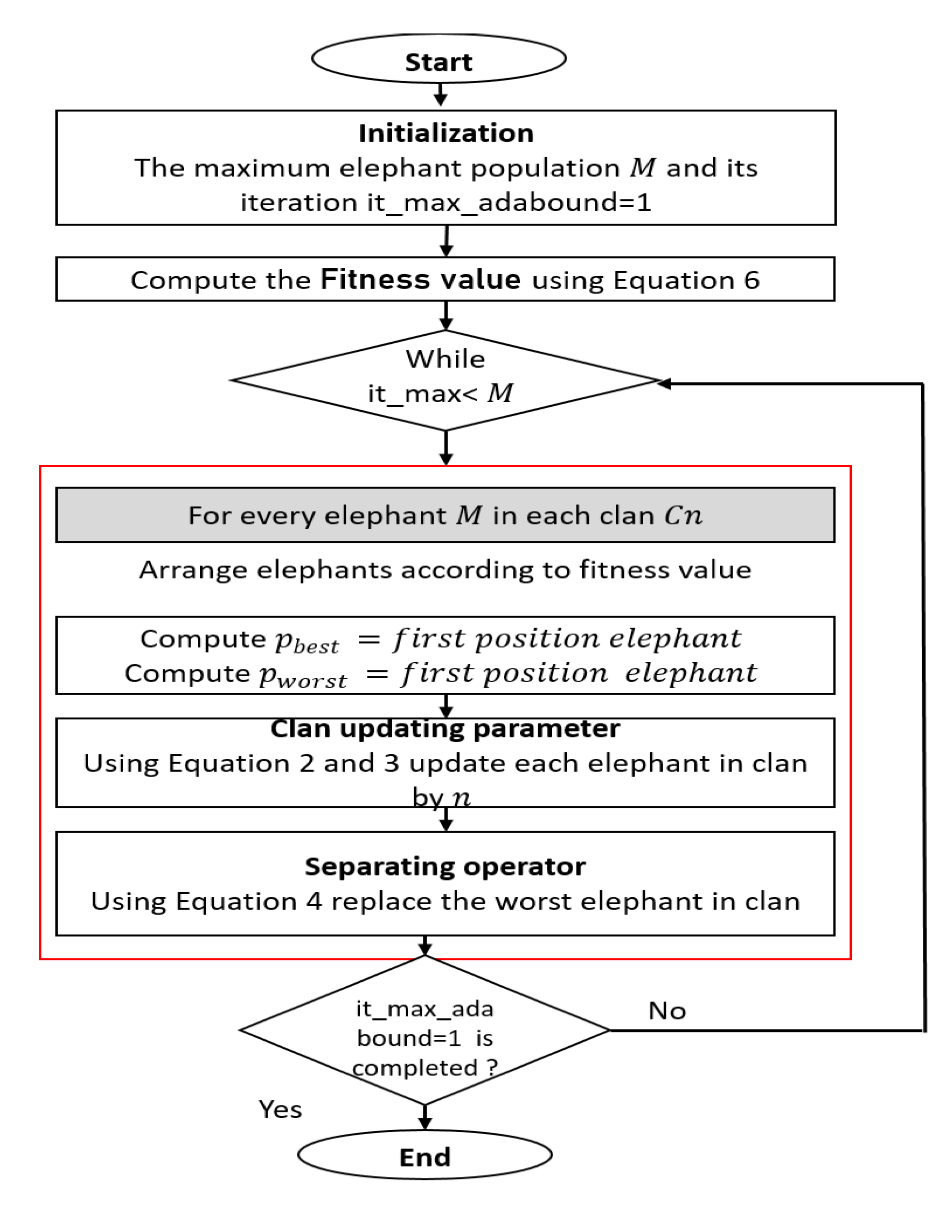
3.1. AdaBound Optimizer as Hyper-Parameter Updating Method in Enhancing EHO

The EHO method is a generalised stochastic search algorithm created by Wang et al. [11] and based on research on elephant behavioural biases. The EHO algorithm is frequently used in machine learning and deep learning optimization. The spatial–spectral hyperspectral image classification in the literature [31] reveals that the modulation classification performance is greatly enhanced using the EHO algorithm to optimise neural networks. The EHO algorithm, on the other hand, contains limitations such as:

• Unreasonable convergence towards the updated operator in the origin has a lower effect on expanding further.
• Initial elephant position allocation is uneven.

For the abovementioned reasons, this paper proposes an enhanced EHO with an AdaBound optimizer. Here, the AdaBound optimizer is used for hyper-parameter updating.

AdaBound Optimizer

To train the proposed CNN model with enhanced EHO, the hyper-parameters are updated using the AdaBound optimizer. The advantage of using the AdaBound optimizer is that it can use dynamic bounds on learning rates to achieve the objective of converting from adaptive to stochastic gradient descent (SGD) optimization, which lowers the generalisation gap between adaptive and SGD approaches with high learning rates. The $\alpha$ is used as the algorithm’s starting step size, and $\alpha /L_t$ is the learning rate. The AdaBound optimizer parameters are updated according to the below equations:

$$h_t=\frac{\partial Q_{i \left(w\right) }}{\partial w}$$

(5)

$$n_t={\beta }_t{n}_{t-1}+\left(1-{\beta }_1\right)h_{t }$$

(6)

$$s_t={\beta }_t{n}_{t-1}+\left(1-{\beta }_1\right){(h_t)}^2$$

(7)

$${{\displaystyle \mathsf{\eta }}}_t=\frac{{\mathsf{\eta }}_t^{\prime }}{\sqrt{t}}$$

(8)

where ${\mathsf{\eta }}_t^{\prime }=clip \left(\alpha /\sqrt{L_t, } {\mathsf{\eta }}_l\left(t\right), {\mathsf{\eta }}_u\left(t\right)\right)$

$$L_t=diag\left(l_t\right)$$

(9)

where the momentum values ${\beta }_1 \mathrm{and} {\beta }_2$ are typically 0.9 and 0.99. $clip \left(\alpha /\sqrt{L_t, } {\mathsf{\eta }}_l\left(t\right), {\mathsf{\eta }}_u\left(t\right)\right)$ denotes that the learning rate $\alpha /L_t$ has been clipped at these values to avoid gradient instability at higher and lower bounds. Instead of a constant lower and upper bound, the hypermeters of ${\mathsf{\eta }}_l$ and ${\mathsf{\eta }}_u$ are specified as functions of $t$. In addition, the parameter update is explained as follows:

$${\omega }_{t+1}=\arg \min {\displaystyle \prod }_{N, Diag\left({\mathsf{\eta }}_t^{\prime }\right)}\left({\omega }_t-{\mathsf{\eta }}_t· n_t\right)$$

(10)

In the above Equation (10), the learning rate is denoted as the function of $t$. Hence, the lower and upper bounds’ limit difference is much lower. According to this characteristic, the above method behaves as Adam at the begining, with bounds having minimal effect on the learning rate. Later, the method behaves as SGD with constrained bounds. With this advantage, AdaBound with new updated hyper-parameters is implemented in EHO to enhance it further. Algorithm 2 presents EEHO with the AdaBound optimizer. The hyper-parameters $\alpha \mathrm{and} \beta$ are considered in the EEHO method, and the initial values of $\alpha \mathrm{and} \beta$ are randomly set within 0 and 1. The convergence rate of the algorithm majorly depends on learning $L_t$; on the other hand, ${\beta }_1 \mathrm{and} {\beta }_2$ have less of an impact on classification accuracy. Thus, this is the factor to improve the performance of classification, by updating the hyper-parameters and enhancing the EHO algorithm. The AdaBound coefficients are set as $L_t$ = 0.001, ${\beta }_1$ = 0.9, and ${\beta }_2$ = 0.999, with a considerable number of iterations. Further, with these updated hypermeters, the minimum error rate is observed; thus, these values are termed as optimal hyper-parameters. In Figure 2, the flow chart of the EEHO–AdaBound is represented.

Algorithm 2: EEHO with AdaBound approach for updating hyper-parameters

# it_max denotes the maximum number of iterations for the EHO algorithm

# it_max_adabound denotes the maximum number of iterations for the AdaBound method

# C_it_adabound denotes the present iteration number of the AdaBound algorithm

# C_it_EHO denotes the present iteration number of the EHO algorithm

# Start Initializations

Initialize the input feature parameters: it_max, it_max_adabound, $L_t$, ${\beta }_1, {\beta }_2,$ and $\alpha$.

Set the present position of elephants

ForC_it_adabound = 1: it_max_adabound

# Develop EEHO

Compute the fitness function of each elephant in the clan

To obtain the best and worst new elephants’ position, calculate and update clan operator

For C_it_EHO = 1: it_max

Equation (1) is used to update the new position of each elephant, respectively

Using Equation (3), evaluate the centre position of elephants

Update the new best value for the elephant’s position using Equation (2)

Calculate the worst value using Equation (4) to update the elephant’s position.

Repeat and evaluate new fitness function for each elephant

The best and worst elephant’s position is recognized

End for

Update the individual elephant’s positions

# End of EHO

Compute ${\omega }_{t+1}$ learning and loss error using Equation (10)

Update the new values for hyper-parameters using Equations (6)–(10).

End for

3.2. The EEHO–CNN Approach

The design of classifiers is a vital aspect of hyperspectral image classification. With the advancement of machine learning, CNN as a classifier has strong self-learning and self-adaptive capabilities and can deal with difficult nonlinear issues. CNN has become widely used in the domain of image classification. This section describes how a convolution neural network based on the enhanced elephant herding algorithm with an AdaBound optimizer is used to classify the hyperspectral images. Figure 3 presents a convolution neural network, in which each node in the network instantly and adaptively selects the distinctive feature and extracts all of the key feature parameters at the same time, ensuring that the image processing accuracy is not limited by the order in which they are used. The CNN classifier in this paper has a three-layer network topology. The number of nodes in the input and output layers is defined by the number of input and output images, respectively. Equation (11) shows how to compute the number of hidden layers’ nodes of the proposed method:

$$\widehat{\rho }=\sqrt{\widehat{r}+\widehat{s} }+k$$

(11)

where $\widehat{r}$ is the number of input features, $\widehat{s}$ is the output features, and $k \left[1,100\right]$ is constant, such that CNN has an integer range of hidden layer nodes from [$\sqrt{\widehat{r}+\widehat{s} }+1, \sqrt{\widehat{r}+\widehat{s} }+100$].

Moreover, the CNN’s preliminary thresholds and weights are set to a different value between −1 and 1, which has an impact on the training duration. With low robustness, this affects the outcomes and convergence results of the CNN. As a result, choosing the best initial weights and thresholds will considerably improve the CNN’s performance. The EEHO with the AdaBound optimizer is used in this paper to optimise the initial threshold values and weights of the CNN.

The input feature set is used to train the CNN in order to predict the system output, and the fitness function’s aim is to minimise the mean absolute error (MAE) between the CNN output layer and the corresponding results. The following describes the optimal solution:

$$f\left(\widehat{\vartheta }\right)=\frac{1}{\widehat{n}} {\displaystyle \sum }_{i=1}^{\vartheta }\left|{\widehat{Y}}_i-P_i\right|$$

(12)

where $\widehat{\vartheta }=\left[{\widehat{\vartheta }}_1, {\widehat{\vartheta }}_2,\dots ,{\widehat{\vartheta }}_D\right]$ is the feature vector that has merged initial weights and threshold values of CNN, such that the weights are set as ${\widehat{\vartheta }}_1=\left[{\widehat{\vartheta }}_1, {\widehat{\vartheta }}_2,\dots ,{\widehat{\vartheta }}_{d1}\right]$ and the threshold value is given by $\widehat{t_1}=\left[{\widehat{\vartheta }}_{d1+1}, {\widehat{\vartheta }}_{d2+2},\dots ,{\widehat{\vartheta }}_{d2}\right]$. Secondly, the features between the input layer and the hidden layers are given by initial weights set to ${\widehat{\vartheta }}_2=\left[{\widehat{\vartheta }}_{d2+1}, {\widehat{\vartheta }}_{d2+2},\dots ,{\widehat{\vartheta }}_{d3}\right]$ and the threshold value set to $\widehat{t_2}=\left[{\widehat{\vartheta }}_{d3+1}, {\widehat{\vartheta }}_{d3+2},\dots ,{\widehat{\vartheta }}_D\right]$, where $d_1=\widehat{n}\times \widehat{\rho }$, $d_2=\widehat{n}\times \widehat{\rho }+\widehat{\rho }$, $d_3=\widehat{n}\times \widehat{\rho }+\widehat{\rho }\times \widehat{r}$, D is the sum of all nodes in the CNN, D is depicted as $D=\widehat{n}\times \widehat{\rho }+\widehat{\rho }+\widehat{\rho }\times \widehat{r}+\widehat{r}$, $\widehat{Y}=\left[{\widehat{Y}}_1, {\widehat{Y}}_2,\dots ,{\widehat{Y}}_n\right]$ is the required expected feature output, and $P=\left[P_1, P_2,\dots ,P_n\right]$ is the predicted output.

The work flow of the CNN based on EEHO with the AdaBound optimizer for HSI classification presented in the proposed approach is shown in Figure 3; the procedural explanation of the design and analysis of the proposed method is as follows:

Step 1: Set the parameters, in which the total number of present elephant groups is $Z,$ the number of elephants $M$, and the number of elephants in each clan $Cn$, $Z=M\times n$ =; the maximum number of group iterations is GenMax. Consider the impact factor $\epsilon ,$ qubit mutation probability $q_1 \mathrm{and} q_{2 ,}$ and the maximum number of iterations Gen. Randomly generate the elephant’s starting position in domain.

Step 2: Using Equation (6), map the best position to the present position; compute the actual fitness value $f\left(\widehat{\vartheta }\right)$ using Equation (7) for each elephant. Depending on the evaluated fitness value provided, arrange the elephants in ascending form. ${\widehat{\vartheta }}_g^t$ is the global fitness value along with the elephant’s new position value.

Step 3: Split all the elephant groups into clans $C$; compute the elephants’ best and worst fitness in $Cn$ clan.

Step 4: Update the clan operator using Equations (1)–(3) to obtain each elephant position.

Step 5: Evaluate the separating operator to replace the individual elephant with its worst case fitness in $Cn$ using Equations (4) and (10).

Step 6: Integrate the elephants of each clan; use Equation (10) to compute each elephant’s fitness value $f\left(\widehat{\vartheta }\right)$. To obtain the elephants’ new location with the global optimal fitness value, organize the elephants in increasing order of their fitness count.

Step 7: Repeat from step 3 until the last elephant obtains the position; otherwise, compute the global position $\widehat{\vartheta }=\left[{\widehat{\vartheta }}_1, {\widehat{\vartheta }}_2,\dots ,{\widehat{\vartheta }}_D\right]$ and stop the algorithm.

Step 8: Once training the network with the best initial thresholds values and weights, the trained CNN models achieve HSI classification accuracy.

4. Experimental Results and Analysis

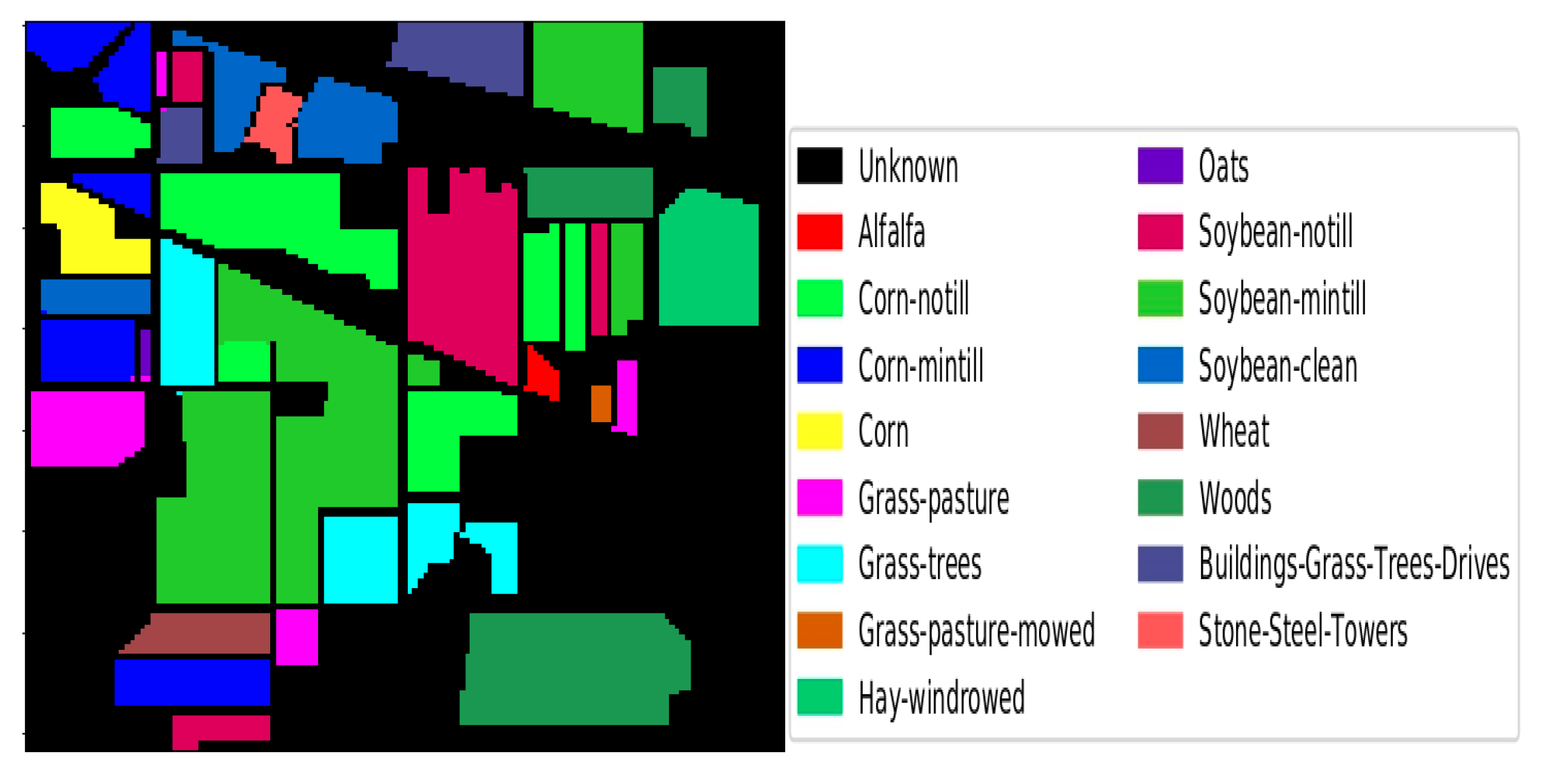
In this section, the experimental setting provided for the proposed method and the parameterized algorithm are explained. Using two HSI datasets, the proposed method for automatically designing CNNs for HSI classification demonstrates the usefulness of the proposed method.

4.1. Dataset

In this section, the proposed method is tested on two standard hyperspectral datasets [33]. Figure 4 presents a diverse vegetation area over the Indian Pines test environment in north-eastern Indiana, USA (Indian Pines), and the Salinas Valley in California, USA (Salinas Valley) (Salinas). The comprehensive data of the training samples of each class are presented in

Table 1. Training and test samples of Indian Pines dataset.

Class Number	Class Name	No. of Training Samples	No. of Test Samples
1	Alfalfa	5	41
2	Corn-not ill	143	1285
3	Corn-mintill	83	747
4	Corn	24	213
5	Grass-pasture	49	434
6	Grass-trees	73	657
7	Grasspasture-mowed	3	25
8	Hay-windrowed	48	430
9	Oats	2	18
10	Soybean-notill	98	874
11	Soybean-mintill	246	2209
12	Soybean-clean	60	533
13	Wheat	21	184
14	Woods	127	1138
15	Buildings-Grass-Trees-Drives	39	347
16	Stone-Steel-Towers	10	83
17	TOTAL	1031	9218

.

From the AVIRIS sensor, a 220-band sensor was used to capture images of the Indian Pines test environment. After removing the water absorption bands, the usable dataset includes a large number of bands (200), with 145 × 145 pixels each. The ground truth map includes 16 different classes of interest.

The second dataset, Salinas, was gathered with the 224-band by the Airborne Visible Infrared Imaging Spectrometer (AVIRIS) over Salinas Valley, California, as shown in Figure 5. It has a spatial resolution of 3.7 m per pixel. After removing the 20 water absorption bands and the 16 land cover classes, the available dataset consists of 204 bands of 512 × 217 pixels.

4.2. Experiments Compared with Existing Approaches

Different CNN classification methods based on spatial–spectral information were used to compare with the proposed method. The CNN–EEHO–AdaBound approach was evaluated in order to assess its performance. To validate the suggested techniques, numerous handmade CNN models with spectral–spatial information were analysed on hyperspectral datasets. The 2D–3D CNN [34] underwent extensive trials with various numbers of training samples, and it was discovered that the CNN model frequently degrades as the sample size decreases. The residual-based approaches to spectral–spatial residual networks (SSRN) [20] and ResNet [35] can obtain better classification accuracy. For contrast, DenseNet [36] was utilised, which exploited shortcut connections between layers of CNN. e-CNN [37], an automatic design analysis method of CNN using AdaBound optimizers to explore the spatial–spectral information, achieved good performance accuracy and was also compared with the proposed method. The existing approaches were compared with previously created CNN models in terms of classification accuracy and computational complexity.

4.3. Experiment Parameter Settings

This section shows the details of the experiment settings, as each dataset was divided into three components in the proposed experiments: a training set, a test set, and a validation set. The training set and validation set proportions of the Indian Pine and Salinas are 5% and 1%, respectively, with the remaining pixels serving as a testing dataset. Table 1 and

Table 2. Training and test samples of Salinas dataset.

Class Number	Class Name	No. of Training Samples	No. of Test Samples
1	Brocoli_green_weeds_1	101	1908
2	Brocoli_green_weeds_2	187	3539
3	Fallow	99	1877
4	Fallow_rough_plow	70	1324
5	Fallow_smooth	134	2544
6	Stubble	198	3761
7	Celery	179	3400
8	Grapes_untrained	564	10,707
9	Soil_vinyard_develop	311	5892
10	Corn_senesced_green_weeds	164	3114
11	Lettuce_romaine_4wk	54	1014
12	Lettuce_romaine_5wk	97	1830
13	Lettuce_romaine_6wk	46	870
14	Lettuce_romaine_7wk	54	1016
15	Vinyard_untrained	364	6904
16	Vinyard_vertical_trellis	91	1716
17	Total	2713	51,416

illustrate the distribution of the sample of the two datasets for each class of their ground truth.

Table 3. The hyper-parameters of CNN–EEHO–AdaBound.

Literals	Considering Parameter	Parameter Value
M	Number of input layer nodes	220
$\widehat{\rho }$	Number of output layer nodes	16
$\widehat{n}$	Number of hidden layer nodes	300
$L_t$	CNN learning rate	0.01
$\widehat{\vartheta }$	CNN training target error	0.001
epochs	CNN maximum number of cycles	100
it_max_adabound	CNN–EEHO maximum number of iterations	50
$Z$	Population size of the quantum elephant herding	30
$C$	Number of clans	5
$C_n$	Number of elephants in each clan	6
$\epsilon$	Influencing factor	0.4

depicts the parameter setting for the proposed CNN–EEHO–AdaBound method.

Whilst carrying out the experiment, the training sets of 2D–3D CNN, SSRN, ResNet, DenseNet, and e-CNN, such as filter size, training epoch, etc., were the same as in the corresponding papers.

5. Results Analysis and Discussion

To demonstrate the usefulness of the proposed method, a study of the classification results is compared in terms of classification accuracy, parameters, and time complexity on benchmark hyperspectral datasets. The proposed method shows the optimal structures and examines the convergence to show that the proposed EEHO with the AdaBound optimizer algorithm is feasible. Finally, testing samples are validated using hyperspectral datasets to promote the effectiveness of CNN–EEHO–AdaBound algorithm techniques.

5.1. Accuracy of HSI Classification

The performance of the models was measured using three metrics: overall accuracy (OA), average accuracy (AA), and Kappa coefficient (Kappa). The ratio of samples properly identified by the model is denoted by OA. The average reliability of all ground objects is denoted by the letter AA. The confusion-matrix indicates the percentage of faults minimised by classification versus an essentially random classification. KAPPA is an accuracy score based on the confusion-matrix.

Table 4. Class-wise overall accuracy (OA%), average accuracy (AA%), and ĸ kappa are represented in the Indian Pines dataset.

Class	2D–3D CNN	SSRN	ResNet	DenseNet	e-CNN	CNN–EEHO–AdaBound
1	71.24	95.26	97.98	99.29	89.79	99.72
2	72.65	95.67	97.63	94.36	97.45	98.64
3	75.13	96.36	96.64	97.58	97.02	97.58
4	87.20	88.83	88.10	99.68	94.32	100.00
5	69.36	97.68	98.57	99.28	95.19	97.64
6	93.57	96.79	100.05	89.57	99.41	100.00
7	64.28	98.25	99.98	100.00	97.23	98.26
8	98.10	99.15	95.14	95.12	99.56	96.76
9	83.13	77.28	94.25	94.50	87.05	98.86
10	77.16	97.79	99.34	96.37	97.34	100.00
11	85.15	98.63	98.28	98.54	99.02	100.00
12	74.87	100.00	100.00	99.01	99.34	97.26
13	98.24	98.38	94.83	100.00	99.67	95.21
14	94.87	99.14	97.28	99.15	99.00	96.84
15	81.89	89.37	89.64	90.16	99.46	88.29
16	77.37	93.48	99.06	89.87	94.93	99.04
OA	83.39	96.91	98.26	99.03	99.36	99.47
AA	82.29	96.06	97.75	98.89	98.81	98.99
ĸ × 100	81.26	95.79	97.78	98.71	97.94	98.32

and

Table 5. Class-wise overall accuracy (OA%), average accuracy (AA%), and ĸ kappa are represented in the Salinas dataset.

Class	2D–3D CNN	SSRN	ResNet	DenseNet	e-CNN	CNN–EEHO–AdaBound
1	94.11	98.46	95.67	99.49	99.67	99.67
2	98.46	96.76	95.79	97.12	98.78	99.39
3	86.03	88.32	92.46	98.63	100.00	98.66
4	98.45	97.68	96.89	98.79	99.12	97.70
5	85.65	92.59	95.26	100.00	98.34	100.00
6	97.68	98.14	89.35	100.00	99.49	100.00
7	95.09	99.06	97.06	99.36	99.37	98.49
8	96.98	75.79	92.37	99.89	99.18	97.71
9	97.12	98.45	98.28	96.78	99.47	98.30
10	77.44	77.60	88.92	97.45	98.31	99.63
11	84.60	79.23	97.56	99.15	98.99	100.00
12	98.36	97.11	100.00	100.00	99.26	100.00
13	97.65	89.98	87.16	98.38	99.46	97.28
14	89.89	88.59	89.03	100.00	99.38	99.18
15	44.23	59.04	91.27	90.45	99.11	92.84
16	85.18	89.11	98.89	97.59	99.98	98.87
OA	90.87	97.15	98.14	99.04	99.01	99.99
AA	89.16	97.56	98.08	99.29	99.19	99.58
ĸ × 100	88.04	95.83	96.51	97.57	97.04	98.12

exhibit the comprehensive classification results on HSI datasets on the proposed method and the other existing methods. As shown in Table 4 and Table 5, CNN with EEHO and the AdaBound Optimizer significantly outperforms previous approaches such as 2D–3D CNN, spectral–spatial residual network (SSRN), residual network (ResNet), dense network DenseNet, and e-CNN in terms of classification accuracy. The proposed method outperformed the other methods in the classification of the Indian Pines dataset. With improvements of 0.11%, 0.18%, and 1.62%, respectively, the CNN–EEHO–AdaBound approach had the best AA and Kappa. The best OA, AA, and Kappa results for the Salinas dataset came from CNN–EEHO–AdaBound, with increases of 0.98%, 0.39%, and 1.08, respectively. There may be significant discrepancies in the accuracy of each class. In the first-class classification on Salinas, CNN–EEHO–AdaBound outperformed 2D–3D CNN by 5.56%.

To summarise the classification accuracy analysis, the proposed CNN–EEHO–AdaBound method outperformed state-of-the-art CNN models such as 2D–3D CNN, SSRN, ResNet, DenseNet, and e-CNN. Using the AdaBound optimizer, the offered methodologies can also identify more optimised architectures. On the other hand, the tuned hyper-parameters resulted in an improved classification performance and reduced computation time.

5.2. Convergence Analysis of CNN–EEHO–AdaBound Approach

In order to significantly speed up optimal value, the convergence analysis of the CNN–EEHO–AdaBound technique must be carried out. The HSI classification accuracy of the optimised convolution neural network, which comprised architectures and biased weight parameters, was used to calculate fitness. The number of architectural characteristics and the position of the elephants, on the other hand, were only related to architecture. As a result, the number of architectural parameters and the position of all elephants were crucial criteria in the CNN–EEHO–AdaBound approach’s architecture convergence study.

The number of hyper-parameters in architectures was inversely proportional to the number of operations in those architectures. The number of hyper-parameters fluctuated as the operations in the models changed, indicating that the designs converged when the number of hyper-parameters remained constant throughout the iterations. The accuracy and number of hyper-parameters of fit during the iterations using the CNN–EEHO–AdaBound technique based on HSI datasets are shown in Figure 6. The architectures converged at seven, nine, and eleven iterations based on the Salinas and Indian Pines datasets, respectively, according to the number of hyper-parameters. After the convergence of the designs, the testing dataset’s accuracy further improved. The fundamental reason for this is that the hyper-parameters of the architectures retained from the EEHO–AdaBound were optimised when CNN was trained until the maximum number of iterations was achieved.

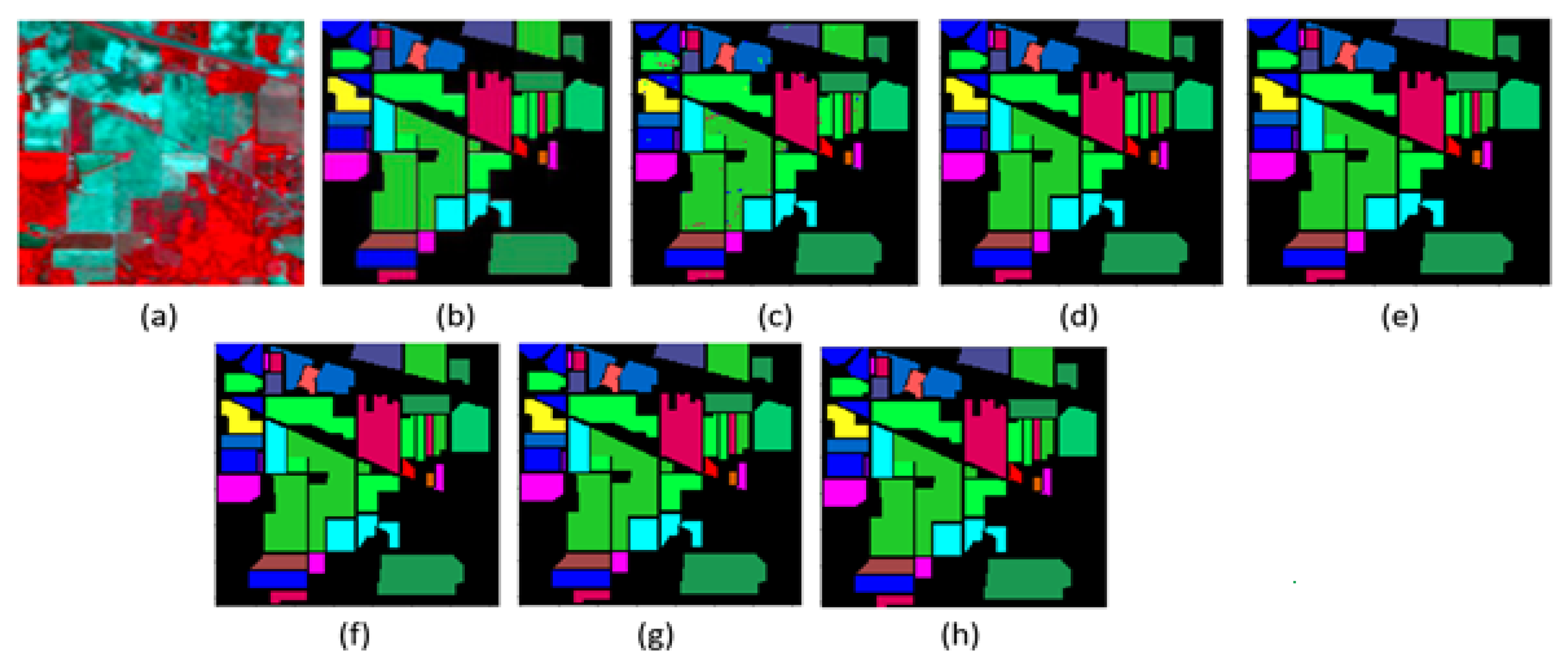
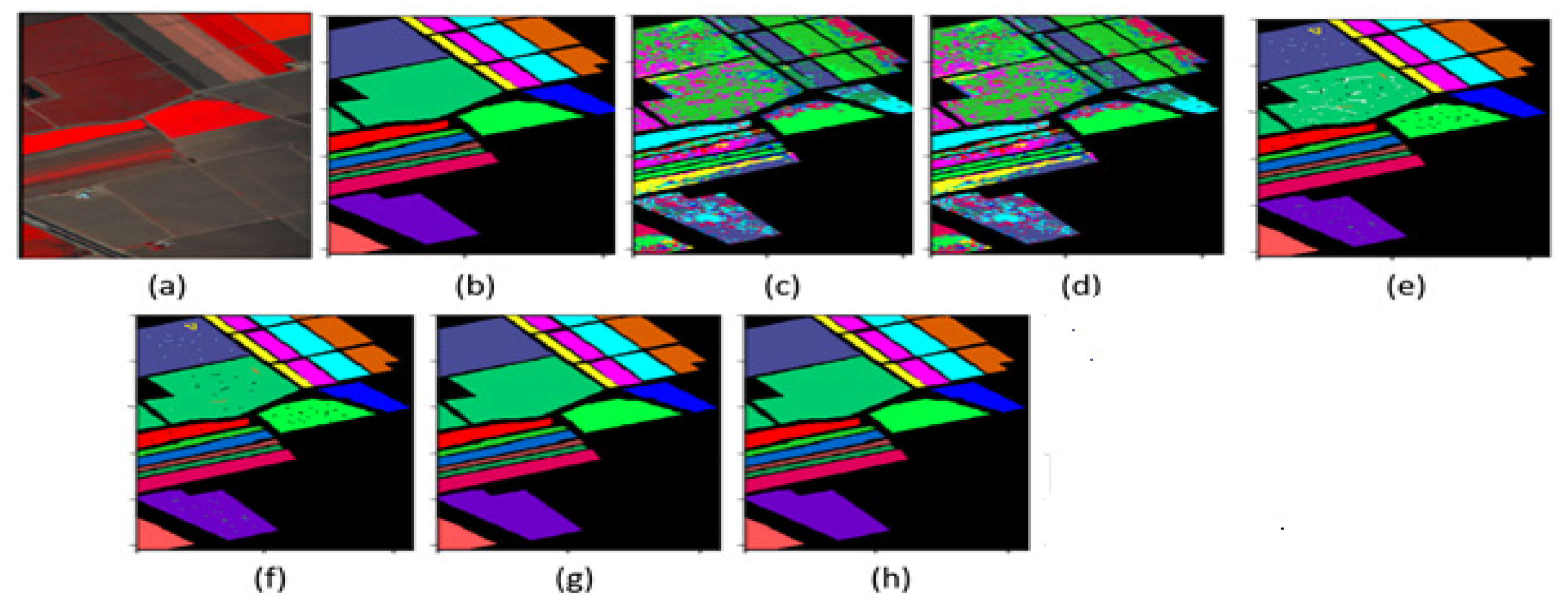
5.3. HSI Classification Maps

The entire HSI image classification maps of all the models effectively represent the classification results. Figure 7 and Figure 8 demonstrate the classification maps generated by several models using two benchmark datasets. In comparison to the other models, the proposed CNN–EEHO–AdaBound produced less dispersion in the class with a wide area, implying that it can achieve more specific classification accuracy in this category. The CNN–EEHO–AdaBound method achieves better results in the classification of various classes in HSI data.

5.4. Comparisons of CNN–EEHO–AdaBound Performance with Other Optimization Algorithms

The PSO–CNN cell-based approach [7], CSO–CNN approach [9], and ACO approach [8] techniques were studied in order to compare the accuracy and effectiveness of the proposed CNN–EEHO–AdaBound and other optimization algorithms. The overall classification accuracy of the four optimization techniques is depicted in

Table 6. Overall accuracy of Salinas dataset with other optimization algorithms.

Performance Evaluation for Indian Pines Dataset	CSO–CNN	ACO	PSO–CNN	CNN–EEHO–AdaBound
OA	91.54	94.61	96.18	99.47
AA	95.49	95.83	96.27	98.99
K × 100	90.53	93.75	95.84	98.32

.

As can be seen in Figure 9, the classification accuracy of the CNN–EEHO–AdaBound method according to the optimization algorithms is significantly higher than that of the existing algorithm, implying that the performance of CNN–EEHO–AdaBound can be enhanced by utilising optimization techniques. The CNN–EEHO–AdaBound method is slightly more precise than other optimization methods, and all of them can achieve greater than 99 percent accuracy. The fundamental reason for this is that these algorithms determine the ideal fitness evaluation value of the individual population, which is a global optimization strategy, decreasing the likelihood of CNN–EEHO–AdaBound that flows into a local minimum. On the other hand, EEHO–AdaBound is an enhancement of the EHO algorithm, with a bio-inspired technique that is very simple to apply and achieves positive efficacy. A faster convergence speed is another advantage of EEHO–AdaBound.

The best optimal fitness value of each optimised generation group of every method is shown in Figure 9, under the condition that the characteristic exponent is $\alpha$ = 1.5. The EEHO–AdaBound algorithm presented in this paper performs much better than the other three algorithms in terms of convergence speed and convergence accuracy, as also shown in Figure 9. As the EEHO–AdaBound is based on the EHO algorithm, it evolves the elephant’s current state with the perfect situation using tuned hyper-parameters. Individuals’ previous metadata are successfully utilised in the evolutionary process, and the algorithm’s global convergence potential is strengthened further.

6. Conclusions

In this research, a high-precision EHO-based algorithm is employed to classify hyperspectral images over CNN using the AdaBound optimizer as a high-speed converging optimizer. The enhanced version of EHO with the AdaBound optimizer method provides much improved classification accuracy by using CNN within it. EEHO–AdaBound outperforms the performance by updating the hyper-parameters. To classify the 16 classes in the HSI dataset, a CNN is optimised using the EEHO–AdaBound approach. The experimental results reveal that the adaptive weight has a good damping impact on the error rate and convergence of the CNN–EEHO–AdaBound approach, considerably improving the accuracy of the HSI dataset. The suggested CNN–EEHO–AdaBound classifier has greatly increased classification accuracy when compared to existing classic CNN classifiers. Furthermore, the EEHO–AdaBound algorithm proposed in this work can improve the EHO’s global convergence competence; when compared to other traditional optimization algorithms, EEHO–AdaBound has a faster convergence speed and higher convergence accuracy, demonstrating its greater versatility and ease of application to other optimization problems. When the hyper-parameters are updated, the CNN–EEHO–AdaBound-based classifier has a maximum classification accuracy of 99.6%. The classification performance measures can be further enhanced in the future by modifying EHO. For the HSI image classification problem, the superiority of the EEHO–AdaBound algorithm in CNN as a technique to update hyper-parameters achieves good performance.

References

1. Lee, H.; Kwon, H. Going deeper with contextual CNN for hyperspectral image classification. IEEE Trans. Image Process. 2017, 26, 4843–4855. [Google Scholar] [CrossRef] [PubMed] [Green Version]
2. Ma, L.; Liu, Y.; Zhang, X.; Ye, Y.; Yin, G.; Johnson, B.A. Deep learning in remote sensing applications: A meta-analysis and review. ISPRS J. Photogramm. Remote Sens. 2019, 152, 166–177. [Google Scholar] [CrossRef]
3. Pan, B.; Shi, Z.; Xu, X. MugNet: Deep learning for hyperspectral image classification using limited samples. ISPRS J. Photogramm. Remote Sens. 2018, 145, 108–119. [Google Scholar] [CrossRef]
4. Yi, C.; Zhao, Y.Q.; Chan, J.C.W. Hyperspectral image super-resolution based on spatial and spectral correlation fusion. IEEE Trans. Geosci. Remote Sens. 2018, 56, 4165–4177. [Google Scholar] [CrossRef]
5. El-Sharkawy, Y.H.; Elbasuney, S. Hyperspectral imaging: Anew prospective for remote recognition of explosive materials. Remote Sens. Appl. Soc. Environ. 2019, 13, 31–38. [Google Scholar] [CrossRef]
6. Junior, F.E.F.; Yen, G.G. Particle swarm optimization of deep neural networks architectures for image classification. Swarm Evol. Comput. 2019, 49, 62–74. [Google Scholar] [CrossRef]
7. Zhang, C.; Liu, X.; Wang, G.; Cai, Z. Particle swarm optimization based deep learning architecture search for hyperspectral image classification. In IGARSS 2020–2020 IEEE International Geoscience and Remote Sensing Symposium; IEEE: New York, NY, USA, 2020; pp. 509–512. [Google Scholar]
8. Sharma, S.; Buddhiraju, K.M. Spatial–spectral ant colony optimization for hyperspectral image classification. Int. J. Remote Sens. 2018, 39, 2702–2717. [Google Scholar] [CrossRef]
9. Sawant, S.S.; Prabukumar, M.; Samiappan, S. A modified Cuckoo Search algorithm based optimal band subset selection approach for hyperspectral image classification. J. Spectr. Imaging 2020, 9, A6. [Google Scholar] [CrossRef]
10. Zhu, X.; Nan, L.; Pan, Y. Optimization Performance Comparison of Three Different Group Intelligence Algorithms on a SVM for Hyperspectral Imagery Classification. Remote Sens. 2019, 11, 734. [Google Scholar] [CrossRef] [Green Version]
11. Wang, G.-G.; Deb, S.; Gao, X.-Z.; Coelho, L.D.S. A New Metaheuristic Optimisation Algorithm Motivated by Elephant Herding Behaviour. Int. J. Bio-Inspired Comput. 2016, 8, 394–409. [Google Scholar] [CrossRef]
12. Santara, A.; Mani, K.; Hatwar, P.; Singh, A.; Garg, A.; Padia, K.; Mitra, P. BASS Net: Band-adaptive spectral-spatial feature learning neural network for hyperspectral image classification. IEEE Trans. Geosci. Remote Sens. 2017, 55, 5293–5301. [Google Scholar] [CrossRef] [Green Version]
13. Kiranyaz, S.; Ince, T.; Abdeljaber, O.; Avci, O.; Gabbouj, M. May. 1-d convolutional neural networks for signal processing applications. In Proceedings of the ICASSP 2019-2019 IEEE International Conference on Acoustics, Speech and Signal Processing (ICASSP), Brighton, UK, 12–17 May 2019; IEEE: New York, NY, USA, 2019; pp. 8360–8364. [Google Scholar]
14. Zhang, M.; Li, W.; Du, Q. Diverse region-based CNN for hyperspectral image classification. IEEE Trans. Image Process. 2018, 27, 2623–2634. [Google Scholar] [CrossRef] [PubMed]
15. Roy, S.K.; Krishna, G.; Dubey, S.R.; Chaudhuri, B.B. HybridSN: Exploring 3-D–2-D CNN feature hierarchy for hyperspectral image classification. IEEE Geosci. Remote Sens. Lett. 2019, 17, 277–281. [Google Scholar] [CrossRef] [Green Version]
16. Sellami, A.; Farah, M.; Farah, I.R.; Solaiman, B. Hyperspectral imagery classification based on semi-supervised 3-D deep neural network and adaptive band selection. Expert Syst. Appl. 2019, 129, 246–259. [Google Scholar] [CrossRef]
17. He, M.; Li, B.; Chen, H. Multi-scale 3D deep convolutional neural network for hyperspectral image classification. In Proceedings of the 2017 IEEE International Conference on Image Processing (ICIP), Beijing, China, 17–20 September 2017; IEEE: New York, NY, USA, 2017; pp. 3904–3908. [Google Scholar]
18. Liu, B.; Yu, X.; Zhang, P.; Tan, X.; Yu, A.; Xue, Z. A semi-supervised convolutional neural network for hyperspectral image classification. Remote Sens. Lett. 2017, 8, 839–848. [Google Scholar] [CrossRef]
19. Zhang, J.; Wei, F.; Feng, F.; Wang, C. Spatial–spectral feature refinement for hyperspectral image classification based on attention-dense 3D-2D-CNN. Sensors 2020, 20, 5191. [Google Scholar] [CrossRef]
20. Zhong, Z.; Li, J.; Luo, Z.; Chapman, M. Spectral–spatial residual network for hyperspectral image classification: A 3-D deep learning framework. IEEE Trans. Geosci. Remote Sens. 2017, 56, 847–858. [Google Scholar] [CrossRef]
21. Jayanth, J.; Shalini, V.S.; Ashok Kumar, T.; Koliwad, S. Land-use/land-cover classification using elephant herding algorithm. J. Indian Soc. Remote 2019, 47, 223–232. [Google Scholar] [CrossRef]
22. Prabowo, A.S.; Sihabuddin, A.; Azhari, S.N. Adaptive moment estimation on deep belief network for rupiah currency forecasting. Indones. J. Comput. Cybern. Syst. 2019, 13, 31–42. [Google Scholar] [CrossRef] [Green Version]
23. Luo, L.; Xiong, Y.; Liu, Y.; Sun, X. Adaptive gradient methods with dynamic bound of learning rate. arXiv 2019, arXiv:1902.09843. [Google Scholar]
24. Strumberger, I.; Minovic, M.; Tuba, M.; Bacanin, N. Performance of elephant herding optimization and tree growth algorithm adapted for node localization in wireless sensor networks. Sensors 2019, 19, 2515. [Google Scholar] [CrossRef] [Green Version]
25. El Shaarawy, I.A.; Houssein, E.H.; Ismail, F.H.; Hassanien, A.E. An exploration-enhanced elephant herding optimization. Eng. Comput. 2019, 36, 3029–3046. [Google Scholar] [CrossRef]
26. Hassanien, A.E.; Kilany, M.; Houssein, E.H.; Hameed, A. Intelligent Human Emotion Recognition Based on Elephant Herding Optimization Tuned Support Vector Regression. Biomed. Signal Process. Control. 2018, 45, 182–191. [Google Scholar] [CrossRef]
27. Li, Y.; Xiao, J.; Chen, Y.; Jiao, L. Evolving deep convolutional neural networks by quantum behaved particle swarm optimization with binary encoding for image classification. Neurocomputing 2019, 362, 156–165. [Google Scholar] [CrossRef]
28. Gao, Y.; Qin, L. A Segmented Particle Swarm Optimization Convolutional Neural Network for Land Cover and Land Use Classification of Remote Sensing Images. Remote Sens. Lett. 2019, 10, 1182–1191. [Google Scholar] [CrossRef]
29. Qiao, H.; Wan, X. Object-Based Classification from Tiangong-2 Using Support Vector Machine Optimized with Evolutionary Algorithm. In Proceedings of the Tiangong-2 Remote Sensing Application Conference; Springer: Singapore, 2019; pp. 222–231. [Google Scholar]
30. Shang, Y.; Zheng, X.; Li, J.; Liu, D.; Wang, P. A comparative analysis of swarm intelligence and evolutionary algorithms for feature selection in SVM-based hyperspectral image classification. Remote Sens. 2022, 14, 3019. [Google Scholar] [CrossRef]
31. Kilany, M.; Hassanien, A.E. A Hybrid Elephant Herding Optimization and Support Vector Machines for Human Behavior Identification. In Proceedings of the 2017 Eighth International Conference on Intelligent Computing and Information Systems (ICICIS), Cairo, Egypt, 5–7 December 2017; pp. 178–184. [Google Scholar]
32. Rajendran, G.B.; Kumarasamy, U.M.; Zarro, C.; Divakarachari, P.B.; Ullo, S.L. Land-use and land-cover classification using a human group-based particle swarm optimization algorithm with an LSTM Classifier on hybrid pre-processing remote-sensing images. Remote Sens. 2020, 12, 4135. [Google Scholar] [CrossRef]
33. Landgrebe, D.A. Available online: http://www.ehu.eus/ccwintco/index.php/Hyperspectral_Remote_Sensing_Scenes (accessed on 17 June 2021).
34. Yu, C.; Han, R.; Song, M.; Liu, C.; Chang, C.I. A simplified 2D-3D CNN architecture for hyperspectral image classification based on spatial–spectral fusion. IEEE J. Sel. Top. Appl. Earth Obs. Remote Sens. 2020, 13, 2485–2501. [Google Scholar] [CrossRef]
35. Feng, F.; Wang, S.; Wang, C.; Zhang, J. Learning Deep Hierarchical Spatial–Spectral Features for Hyperspectral Image Classification Based on Residual 3D-2D CNN. Sensors 2019, 19, 5276. [Google Scholar] [CrossRef] [PubMed] [Green Version]
36. Paoletti, M.; Haut, J.; Plaza, J.; Plaza, A. Deep&Dense convolutional neural network for hyperspectral image classification. Remote Sens. 2018, 10, 1454. [Google Scholar]
37. Kavitha, M.; Gayathri, R.; Polat, K.; Alhudhaif, A.; Alenezi, F. Performance Evaluation of Deep e-CNN with Integrated Spatial-Spectral Features in Hyperspectral Image Classification. Measurement 2022, 191, 110760. [Google Scholar] [CrossRef]
Figure 1. Elephant behaviour in a clan.
Electronics 12 01157 g001
Figure 2. Flow chart of enhanced EHO with AdaBound optimizer.
Electronics 12 01157 g002
Figure 3. The CNN–EEHO–AdaBound flowchart for HSI classification.
Electronics 12 01157 g003
Figure 4. Indian Pines dataset with colour codes.
Electronics 12 01157 g004
Figure 5. Salinas dataset with colour codes.
Electronics 12 01157 g005
Figure 6. The training convergence performance.
Electronics 12 01157 g006
Figure 7. Indian Pines classification maps. (a) RGB image; (b) ground truth; (c) 2D–3D CNN; (d) SSRN; (e) ResNet; (f) DenseNet; (g) e-CNN; and (h) CNN–EEHO–AdaBound.
Electronics 12 01157 g007
Figure 8. Salinas classification maps. (a) RGB image; (b) ground truth; (c) 2D–3D CNN; (d) SSRN; (e) ResNet; (f) DenseNet; (g) e-CNN; and (h) CNN–EEHO–AdaBound.
Electronics 12 01157 g008
Figure 9. Overall accuracy for optimization algorithms.
Electronics 12 01157 g009