Abstract
For the ultra-wideband chaotic radio pulses an analytical model of an energy detector is designed and closed-form expressions for the optimal threshold and the detection probabilities are derived. The analytical solution is compared with the results of the numerical simulation. The model proves to be well-suited for the chaotic radio pulses with large base B (or processing gain, or the number of freedom degrees), namely, B ≥ 100. Potential applications areas of the proposed model are ultra-wideband communications with chaotic pulse carriers, e.g., ultra-wideband systems of 802.15.x standards, and multi-element chaotic communication systems.
1. Introduction
Designing communication devices usually requires tedious numerical simulation. Occasionally, analytical solutions can be derived, exact or approximate, that allow us to substitute numerical simulation by direct calculation of analytical formulas, which can simplify and accelerate the design procedure. However, efficient analytical solutions pertain, as a rule, to concrete schemes, signals, and processing algorithms, because they take into account the signal statistics, the circuit or algorithm peculiarities, etc.; that is, they are not universal, and the introduction of a new type of, e.g., information carrier may require a new analytical solution.
Such an introduction of ultra-wideband (UWB) signals at the beginning of the 2000s [1] and the development of communications based on such signals, in particular direct chaotic communications [2], raised interest in analytical models of the energy detector (ED) [3,4,5,6,7,8,9]. Much interest in using energy detectors is now paid to MIMO (multiple input – multiple output) systems, including UWB MIMO systems [10,11,12,13].
The history of analytical ED models started long ago [14,15,16,17,18], and many solutions were presented since then. The structure of these models is approximately the same. As a rule, they contain a block for estimating the signal energy and a decision unit that makes a conclusion on the received information. The energy estimation function is implemented by the “squaring device + integrator” bundle, which corresponds to the “diode + LPF” (low-pass filter) radio components. With regard to digital communications, the energy of a radio pulse encoding a certain symbol is estimated on a certain time interval and, based on the energy value, the ED decides that one of several symbols is received. In the case of binary communications, the decision is usually made by comparing the energy value with a threshold (single-sample detection) [17,18]. Often the choice of the threshold and its optimal value are also a part of the model.
After the signal energy is evaluated, information about the type of the data carrier (regular, pseudo-noise, AM, FM, etc.) is lost, and its nature exhibits itself only in the statistics of the energy values corresponding to transmitted symbols. In many cases, these statistics are close to random, and they can therefore be approximated by a normal distribution due to the central limit theorem (CLT) [18]. An analysis of the literature shows that such a transition to an approximate solution is a very popular approach [17,18,19,20,21,22,23,24,25,26].
To date, in addition to many existing ED models, new ones constantly appear to solve still newer tasks. For instance, optimization of the signal sampling time (or the number of sensed samples) is analyzed in [19] for the problem of spectrum sensing under the effect of noise uncertainty, and a CLT-based ED model is used to compute the signal detection and false alarm probabilities. Energy detection in the case of a signal with a random amplitude is investigated in [20] for various amplitude statistics (Rayleigh, Rice, Nakagami, etc.); distributions of ED decision statistics are retrieved and expressions for detection probabilities are obtained.
The authors of [21] notice that “the performance analysis of ED over slow fading channels is cumbersome, because it is difficult to derive closed-form expressions for the average probability of detection…”; in order to obtain a computationally tractable solution, they derive an approximation “by replacing the log-normal distribution with a Wald distribution”; as for the ED, they count on [22], which gives a direct Q-form solution for the χ2-distribution.
In Ref. [23], the author invents novel signal-processing techniques to improve the detection performance by choosing the value of the power operation of the signal sample according to the system settings; under certain conditions “new energy detectors outperform the conventional energy detector.” ED for baseband sampling is derived in [24], where detection and false alarm probabilities are calculated using a CLT approximation for the χ2-distribution; the motivation is that for N > 200 “the Marcum Q-function is difficult to calculate or to take its inverse.”
ED models are derived in [25] for various signal distributions that actually correspond to different wireless channels (multipath, fading, etc.); the author uses CLT and claims to have obtained more accurate approximations of the test signal statistic. In [26], instead of using CLT to proceed to normal distribution, the authors use more complex approximations of χ2-distribution, which improves the accuracy of ED performance by several percent.
Energy detectors are also widely used, and their models are designed in fiber optics and visible light communications (VLC), e.g., [27,28,29].
In this paper, we propose an analytical model for the energy detector of ultra-wideband chaotic radio pulses. Such a detector is a part of the scheme of Direct Chaotic Communications (DCC) [2], which is the only practical implementation of chaotic communications at the moment. Early days of chaotic communications were associated mostly with chaotic synchronization [30,31]; however, this phenomenon proved to be delicate and sensitive to signal distortion in the channel. Since classical correlation receivers are very difficult (if possible) to apply to chaos, differential correlation methods have been proposed, such as DCSK (differential chaos shift keying) [32,33], in which the reference signal is transmitted along with the modulated signal through the same channel. The practical realization of DCSK systems has met technical difficulties (e.g., lack of long UWB time-delay components); therefore, at present such systems are mostly a subject of theoretical studies.
Direct chaotic communications are based on the following ideas: the communication circuit must be as simple as possible, so the chaotic oscillations must be produced, modulated, and demodulated directly within the same frequency band that is given for the communication channel; no chaotic synchronization, because of its low immunity to the signal distortion; no up-and-down frequency conversion; and an incoherent receiver [34]. The transmitted information is encoded with a stream of chaotic radio pulses. The main element of this scheme, a chaotic radio pulse, has a number of unique features: it is wideband or ultra-wideband by origin, because it is a property of the oscillations of the dynamic system which can be reliably controlled; variation of the pulse duration T has little or no effect on its spectrum; autocorrelation time of the UWB pulse is extremely small because it is inversely proportional to frequency bandwidth Δf; the base of the pulse (or the number of its freedom degrees) B = 2Δf·T ≫ 1; and it can be varied arbitrarily by simply adjusting the pulse duration T (in contrast, another popular UWB signal, an ultrashort pulse, is an elementary signal with the base B = 1).
Here we derive an analytical model of the energy detector of UWB chaotic radio pulses (Figure 1) in the static AWGN (additive white Gaussian noise) channel. The system behavior in a multipath environment needs special consideration; some of its aspects were investigated numerically in [34].
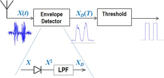
Figure 1.
Energy detector of chaotic radio pulses.
The structure of this paper is as follows. In Section 2, we describe the energy detector and the received signal transformation; we discuss chaotic signal models and derive approximate expressions for the BER (bit error ratio) and the optimal threshold. In Section 3, we compare the analytical BER values with the results of numerical simulation. In Section 4, we discuss the accuracy of the proposed model and analyze its limits and its applicability to other types of UWB signals. In the conclusion, we summarize the obtained results and point at potential applications of the ED model.
2. Energy Detector Model
Here we consider an orthogonal system of signals, also called OOK (on-off keying) or ASK (amplitude shift keying), in which symbol ‘1’ is encoded by a radio pulse on a prescribed time interval, and symbol ‘0’ by no pulse on that time interval. In our case, the task of the energy detector is to detect the presence of a UWB radio pulse against an AWGN background.
The detector is assumed quadratic (square-law), non-quadratic detectors are discussed in Section 4.
2.1. Signal Processing in the Envelope Detector
Let us describe the signal transformation in the receiver. The schematic of the envelope detector is represented with a quadratic diode and a low-pass filter (LPF) (Figure 1), i.e., a squaring device and an integrator (a band-pass filter at the input is not shown, yet it is implied).
An RF (radio frequency) UWB electric signal at the detector input is denoted as X(t). To detect a radio pulse on a time interval, which we denote for certainty as [0, T], where T is the radio pulse duration, the detector must distinguish between the two cases:
where s(t) is a carrier chaotic signal generated by a deterministic dynamic system whose spectrum S(f) is confined in the frequency band [flo, fup], and ξ(t) is the AWGN of the same frequency band [flo, fup].
| X1(t) = s(t) + ξ(t), | —symbol ‘1’ (a radio pulse), |
| X0(t) = ξ(t) | —symbol ‘0’ (no pulse), t ∈ [0, T], |
From the output of the squaring device (a diode), the signal X2(t), that is the instantaneous power of the received signal, is fed to the integrator (a low-pass filter). At its output, the signal is proportional to the energy of the input signal in some preceding time windows Tw.
The filter constant must be matched with the pulse length T; therefore, if the voltage across the filter output is sampled at moment T, when the filter window coincides with the interval [0, T], then the envelope detector sample XD(T) is equal to the radio pulse energy on the interval [0, T]. That is, XD(T) = E1 when transmitting symbol “1” or XD(T) = E0 when transmitting symbol “0”. Hereinafter, the subscripts “1” or “0” of the variables and functions refer to the cases of pulse and no pulse, respectively.
Let us expand the expression for E1
Chaotic signal s(t) and noise ξ(t) are uncorrelated zero-mean variables; hence, the cross-correlation term in (2) is close to zero and can be discarded.
Following the usual approach, we proceed from continuous to discrete signal representation:
Here, si and ξi are independent samples on [0, T]. Since the continuous signals occupy a frequency band [flo, fup], according to the sampling theorem, the samples must be taken in time intervals Δt = 1/2Δf = 1/2(fup − flo). The number of independent samples (number of freedom degrees) on the pulse interval is n = T/Δt = 2TΔf = B, where B = 2Δf·T is the signal base (processing gain).
Similarly, energy E0 in expression (4) is the sum of the squares of random noise samples ξi. Here we describe AWGN samples with a normal distribution N(0,). Accordingly, the sums of the squares of such samples have noncentral χ2-distribution with n degrees of freedom with math expectation E[χ] = n and variance D[χ] = . In agreement with the central limit theorem [18], at n → ∞ this χ2-distribution tends to a normal distribution N(n, 2n). In practice, DCC systems operate with the bases B = 100–250 and more [34,35], so condition n ≫ 1 is fulfilled. With good accuracy, we can approximate E0 with the expression:
where ζnoise is described by a zero-mean distribution N(0, 2n
).
2.2. Models of Chaotic Signals
As was mentioned earlier, after calculating (or measuring) the energy of the radio pulse, information about the nature of the information carrier (chaotic, regular, modulation type, etc.) is actually lost. However, it exhibits itself in the statistic of E1. Radio pulses are usually described with three variables: amplitude, frequency, and phase. Chaotic radio pulses (i.e., fragments of chaotic oscillations generated by a nonlinear dynamic system) can be chaotic in every pulse variable. For example, some chaotic systems give chaotic-phase oscillations with nearly constant amplitude, so they are usually referred to as “phase chaos” [36,37]. However, the most common are the chaotic signals, in which amplitude, phase, and frequency are chaotic all together; they are usually called “amplitude chaos” (e.g., [38,39]). These types of chaotic signals and the corresponding models of such signals were analyzed in [40,41], where the performance of communication systems was estimated by means of numerical modeling.
Three statistic models of a band-limited chaotic signal were investigated: (a) a “telegraph”, (b) a Gaussian, and (c) a uniform [40]. The “telegraph” signal, whose samples are a random sequence of “–1” and “1”, is a model of the phase chaos, i.e., oscillations with a constant amplitude but a chaotically oscillating phase. It is easy to see that in this case, the energy of radio pulses is practically constant, and its statistic is indistinguishable from the statistic of classical radio pulses with a sinusoidal filling. The second signal model, a band-limited Gaussian noise, is used to describe the general chaotic-amplitude type of signals, in which all three oscillation variables are chaotic. Despite the general nature of this model, it does not fully correspond to practically feasible chaotic signals, since it allows arbitrarily large (albeit improbable) amplitudes, whereas the signals of real physical systems cannot take on infinite values. To achieve a better fit, the authors of [40] proposed a third model that represented a random signal whose samples have a limited uniform distribution.
In chaotic communications, the “phase chaos” was shown to provide better BER than the “amplitude chaos”, because pulse-to-pulse energy variations of the phase-chaotic signal are insignificant due to nearly constant amplitude, whereas for chaotic-amplitude pulses such variations are essential, which adds interference to the system noise [40,41].
In this study, we consider the “amplitude chaos” model as a more general case.
Chaotic signal si with a flat spectral characteristic with good accuracy can be modeled with a white noise of the same frequency band [flo, fup]; therefore, its samples can be described with a normal distribution . Consequently, a noncentral χ2-distribution for E1 (3) can also be approximated by a normal distribution, i.e.:
where ζΣ are samples with normal distribution
or, in a simpler form,
, where .
2.3. Energy Statistics and Optimal Threshold
Thus, we approximated the energy sample statistics with the following functions:
where and are the average energy of the received signal on the interval [0, T] in the absence and in the presence of radio pulse, respectively. These functions are shown schematically in Figure 2.
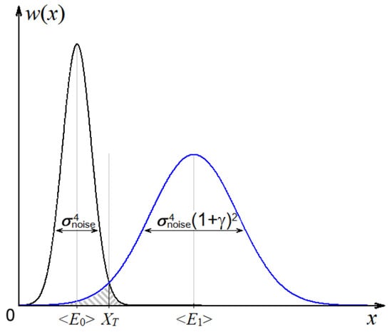
Figure 2.
Energy distribution functions for symbols “0” and “1”.
To distinguish the received symbols, let us introduce a pulse energy threshold XT, such that the received symbol is “0,” if XD sample at the output is below the threshold, i.e., XD(T) < XT; otherwise, the received symbol is “1”.
We define the detection error probability Perr as the sum of the error probabilities for each of the two binary symbols. To evaluate Perr, we calculate the hatched area in Figure 2. If the binary symbols “0” and “1” are transmitted with probabilities p(0) and p(1), then:
The optimal threshold is obtained by means of minimizing the functional Perr(x), which gives the following equation for XT:
To solve Equation (9), we expand functions w0 (6) and w1 (7)
take a natural logarithm of both sides
introduce a new variable , and, after rearrangement, obtain a quadratic equation:
Equation (12) has two real roots, a negative one, which we discard, and a positive one, which gives us an explicit expression for the optimal threshold:
Here, parameter B = 2Δf·T is the base (processing gain, number of freedom degrees) of the signal, and can be treated as a sort of signal-to-noise ratio (SNR) at the receiver input. Actually, in the case p(0) = p(1) = 0.5, , because the average signal power Pchaos is half the pulse power.
In order to simplify further expressions, we introduced . In Figure 3 a bunch of YT curves corresponding to different values of B is plotted (p(0) = p(1) = 0.5). As can be seen, for large B (>100) the optimal threshold value YT is confined in the range 1 ≤ YT ≤ 2. The larger B, the less the discrepancy between the curves, so that for B ≥ 1000 the threshold becomes practically independent of B. Additionally, since the most interesting range of SNR is [–10…0 dB] (see Figure 4), it seems that expression (13) could further be approximated by some simpler formula.
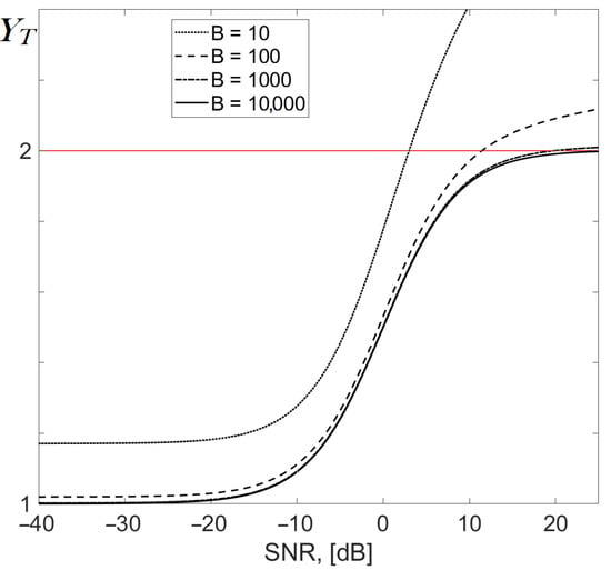
Figure 3.
Threshold YT as a function of SNR for various values of the processing gain B.
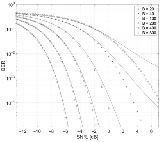
Figure 4.
BER as a function of SNR and processing gain B. Solid lines correspond to simulation; dotted curves to analytical estimates (15).
2.4. Detection Probability
Knowing the optimal threshold value, we obtained the following analytical solution for the receiver probability error in the case of ultra-wideband chaotic radio pulse with a large processing gain B ≫ 1:
where is the complementary CDF (cumulative distribution function) of the normal distribution.
Using the previously introduced and employing the symmetry of w1(x), we get the final expression for BER:
False alarm probability PFA can be defined as the probability of detecting symbol “1” instead of actually transmitted symbol “0”. Then, this probability is:
3. Comparing Analytical and Simulation Probabilities
Let us compare theoretical estimates (15) and (16) with the results of numerical simulation. In Figure 4, BER values are depicted as functions of SNR. Marked plots represent direct BER calculations. To get these plots for a given value of SNR, we acquired statistics of E0 and E1 for 106–107 chaotic radio pulses of base B, then we evaluated the area under the overlapping “tails” of the distributions (the shaded regions in Figure 2); cumulative probability distribution function (CPF) was more convenient than PDF (probability distribution function) in this task. Symbol probabilities were equal, i.e., p(0) = p(1) = 0.5. The curves running through marked plots depict corresponding theoretical estimates (15).
As can be seen, for small values of the signal base B analytical and numerical plots quickly diverge with increasing SNR, which means that for small values of B, the theoretical estimates (15) are not very good.
However, for large B the discrepancy is negligible. This discrepancy is explained by the approximation of χ2-distribution by the normal distribution, the accuracy of which increases with B = n → ∞ (more details in the next Section). The question is when this approximation can be considered effective. As can be seen in Figure 4, beginning from B = 100, the SNR difference between the actual and approximate plots becomes acceptable, e.g., for BER = 10−4, it is less than half dB.
To proceed from BER as a function of SNR to a more usual function BER(Eb/N0), one should follow these simple transformations:
where Eb is the average bit energy; Tb is the pulse duration; N0 is the AWGN spectral density; Δf is the UWB signal frequency bandwidth; and B = 2Δf·Tb is the signal base (processing gain, number of freedom degrees) hence:
One should note that expression (18) is derived under the assumption of equal probabilities of binary symbols “0” and “1”, so the average signal energy Eb is half the average pulse energy E1.
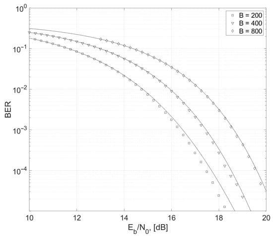
Figure 5.
BER as a function of Eb/N0 and processing gain B.
Thus, for B > 100, the presented energy detector model allows an evaluation of the error probability with an accuracy that is sufficient for engineering calculations.
4. Discussion
In order to understand the reason for the discrepancy between the analytical and the simulation curves in Figure 4 and Figure 5, the function of a χ2-distribution and its approximation by the normal distribution should be considered.
In Figure 6 overlapping χ2-distributions for E0 and E1 obtained in numerical simulation (solid-color areas) are presented along with the two curves that depict the normal distributions that approximate them. For clarity, the distributions are depicted in logY scale.
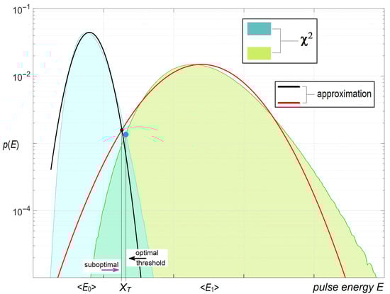
Figure 6.
χ2-distributions and their approximations for E0 and E1.
The optimal threshold that ensures the minimum of Perr is the solution to (9), i.e., the point of intersection of the two distribution functions. As can be seen, the normal distribution functions are symmetric, whereas the functions of noncentral χ2-distributions are tilted to the left. For this reason, the point of intersection of the two approximating normal distributions never coincides with the point of intersection of the χ2-distributions; it is always shifted to the left, thus giving a suboptimal threshold.
As can be seen in Figure 6, normal distributions fit the vertex area of χ2-distributions sufficiently well, but the farther from the vertex, the greater the discrepancy between the χ2 and normal distributions. This is what we see clearly in Figure 4 for small values of B. Therefore, at large values of SNR, when the point of the distributions’ intersection shifts farther and farther towards the “tails”, the “approximate” threshold shifts farther from the optimal one. This is a key moment that is connected with the accuracy of the approximation, and it cannot be corrected other than using either χ2-distribution itself or using distributions the form of which approximates χ2 better than the normal distribution.
In this paper, we considered an energy detector with quadratic characteristics (its squaring device can be implemented, e.g., with a semiconductor diode). However, the described model can also be applied to the log detector. In practice, a log detector is technically more advantageous, since it has a much greater dynamic range. The voltage at the output of the log detector is proportional to the logarithm of the input power. However, the statistic of the log detector output values remains random-like, and due to the CLT, it also tends to a normal distribution. Simulation shows that even the outlook of the distribution functions in Figure 2 is preserved (only the Y axis is scaled). Obviously, all further mathematics hold and the results of the above model also describe the performance of the log detector.
When talking about the applicability of this model to other types of UWB signals, such as ultrashort pulses or chirps, we must keep in mind that all of them are signals with fixed waveforms; therefore, the variance of the energy of such pulses is close to zero and the statistic of E1 energy values is determined only by the AWGN variance .
In the 802.15.4a standard, in order to increase the transmission energy, the symbols are encoded by trains of ultrashort pulses, not the single pulses; in order for the spectrum of the emitted signal to be continuous, the pulses are put in random positions within the train (i.e., on the symbol time interval), and their polarity is also set randomly. As can be seen, both “randomization” methods do not change the energy of the emitted signal, so the statistic of the pulse energy values in the receiver of ultrashort pulses is determined mostly by the internal noise of the receiver. Thus, the models of energy detectors for these types of UWB signals can be taken from the bank of narrowband models.
5. Conclusions
In this paper, for the first time, we designed and investigated an analytical model of the energy detector for ultra-wideband chaotic radio pulses with a large base.
Ultra-wideband nature of the chaotic signal allowed us to model it with normally distributed random values. The large base (number of freedom degrees) of chaotic radio pulses justified application of the central limit theorem to the statistic of the radio pulse energy, so it was also described with a normal distribution. These approximations allowed us to get closed-form expressions for the performance of the energy detector (the detection and false alarm probabilities, and the optimal threshold).
The area of application of the proposed model is, first of all, ultra-wideband communications based on chaotic radio pulses. For engineering problems, the applicability bound of this model can be expressed as , because in this case for the error probability Perr = 10−4, the numerical and analytical SNR estimates differ by less than 0.5 dB, which is quite sufficient. This bound can also be expressed through the data rate R since the pulse duration T is related to the transmission rate R as:
hence, the model better suits the relatively low-rate communications. For example, for Δf = 500 MHz and B = 100 the lower bound of the data rate is Rmin = 10 Mbps, whereas Δf = 2000 MHz and B = 100, Rmin = 40 Mbps. (Note that this bound is not for the energy detector, but only for the applicability of the discussed model. The energy detector is certainly functional at the frequencies below this bound, but the model describes it less accurately.) Of the modern wireless communication systems, this model most closely matches the systems of the standards 802.15.4a (optional solution) or 802.15.6.
The obtained analytical solution can facilitate the design of communication systems with a chaotic carrier, in particular, of multi-element systems, by means of replacing tedious numerical simulation with direct calculation.
Funding
This research was done in terms of the State Assignment of the Kotelnikov Institute of Radio Engineering and Electronics of the Russian Academy of Sciences.
Data Availability Statement
Not applicable.
Conflicts of Interest
The author declares no conflict of interest.
Abbreviations
The following abbreviations are used in this manuscript.
| AM | Amplitude modulation |
| ASK | Amplitude shift keying |
| AWGN | Additive white Gaussian noise |
| BER | Bit-error ratio |
| CDF | Cumulative distribution function |
| CLT | Central limit theorem |
| DCC | Direct chaotic communications |
| DCSK | Differential Chaos Shift Keying |
| ED | Energy detector |
| FM | Frequency modulation |
| LPF | Band-pass filter |
| MIMO | Multiple Input–Multiple Output |
| OOK | On-Off keying |
| Probability distribution function | |
| RF | Radio frequency |
| SNR | Signal-to-noise ratio |
| UWB | Ultrawideband |
| VLC | Visible-light communications |
References
- Federal Communications Commission. FCC 02-48—Revision of Part 15 of the Commission’s Rules Regarding Ultra-Wideband Transmission Systems, FIRST REPORT AND ORDER. 2002. Available online: http://www.fcc.gov/Bureaus/Engineering_Technology/Orders/2002/fcc02048.pdf (accessed on 1 October 2022).
- Dmitriev, A.S.; Kyarginsky, B.Y.; Panas, A.I.; Starkov, S.O. Experiments on ultra wideband direct chaotic information transmission in microwave band. Int. J. Bifurc. Chaos 2003, 13, 1495–1507. [Google Scholar] [CrossRef]
- Kockaya, K.; Develi, I. Spectrum sensing in cognitive radio networks: Threshold optimization and analysis. J. Wirel. Commun. Netw. 2020, 2020, 255. [Google Scholar] [CrossRef]
- Atapattu, S.; Tellambura, C.; Jiang, H. Energy Detection for Spectrum Sensing in Cognitive Radio; SpringerBriefs in Computer Science; Springer: New York, NY, USA, 2014. [Google Scholar] [CrossRef]
- Rabbachin, A.; Quek, T.Q.; Pinto, P.C.; Oppermann, I.; Win, M.Z. Non-Coherent UWB Communication in the Presence of Multiple Narrowband Interferers. IEEE Trans. Wirel. Commun. 2010, 9, 3365–3379. [Google Scholar] [CrossRef]
- Nagaraj, S.; Rassam, F.G. Improved Noncoherent UWB Receiver for Implantable Biomedical Devices. IEEE Trans. Biomed. Eng. 2016, 63, 2220–2225. [Google Scholar] [CrossRef] [PubMed]
- Ghozzi, M.; Dohler, M.; Marx, F.; Palico, J. Cognitive radios: Methods for detection of free bands. C. R. Phys. 2006, 7, 794–805. [Google Scholar] [CrossRef]
- Messaadi, M.; Teguig, D.; Sadoudi, S.; Ouslimani, A.; Mesloub, A. GoF Based Chaotic On-Off Keying: A New Non-Coherent Modulation for Direct Chaotic Communication. J. Commun. Technol. Electron. 2021, 66 (Suppl. S2), 194–200. [Google Scholar] [CrossRef]
- Khan, M.G.; Sallberg, B.; Nordberg, J.; Claesson, I. Robust Weighted Non-Coherent Receiver for Impulse Radio UWB PPM Signals. IEEE Commun. Lett. 2011, 15, 614–616. [Google Scholar] [CrossRef]
- Wang, F.; Tian, Z.; Sadler, B.M. Weighted Energy Detection for Noncoherent Ultra-Wideband Receiver Design. IEEE Trans. Wirel. Commun. 2011, 10, 710–720. [Google Scholar] [CrossRef]
- Jing, L.; Utkovski, Z.; de Carvalho, E.; Popovski, P. Performance limits of energy detection systems with massive receiver arrays. In Proceedings of the 2015 IEEE 6th International Workshop on Computational Advances in Multi-Sensor Adaptive Processing, Cancun, Mexico, 13–16 December 2015. [Google Scholar] [CrossRef]
- Sharma, S.; Bhatia, V.; Gupta, A. Noncoherent IR-UWB Receiver Using Massive Antenna Arrays for Wireless Sensor Networks. IEEE Sens. Lett. 2018, 2, 1–4. [Google Scholar] [CrossRef]
- Manolakos, A.; Chowdhury, M.; Goldsmith, A. Energy-Based Modulation for Noncoherent Massive SIMO Systems. IEEE Trans. Wirel. Commun. 2016, 15, 7831–7846. [Google Scholar] [CrossRef]
- Kaplan, E.L. Signal-Detection Studies, with Applications. BSTJ 1955, 34, 403–437. [Google Scholar] [CrossRef]
- Marcum, J. A statistical theory of target detection by pulsed radar. IRE Trans. Inf. Theory 1960, 6, 59–267. [Google Scholar] [CrossRef]
- Urkowitz, H. Energy detection of unknown deterministic signals. Proc. IEEE 1967, 55, 523–531. [Google Scholar] [CrossRef]
- Scharf, L.L. Statistical Signal Processing: Detection, Estimation and Time Series Analysis; Addison-Wesley: Reading, MA, USA, 1991. [Google Scholar]
- Kay, S.M. Fundamentals of Statistical Signal Processing: Detection Theory, 1st ed.; Prentice-Hall: Upper Saddle River, NJ, USA, 1998. [Google Scholar]
- Mahendru, G.; Shukla, A.; Banerjee, P. A Novel Mathematical Model for Energy Detection Based Spectrum Sensing in Cognitive Radio Networks. Wirel. Pers. Commun. 2020, 110, 1237–1249. [Google Scholar] [CrossRef]
- Kostylev, V. Energy detection of a signal with random amplitude. In Proceedings of the 2002 IEEE International Conference on Communications, New York, NY, USA, 28 April–2 May 2002. [Google Scholar] [CrossRef]
- Sun, H.; Laurenson, D.I.; Wang, C.-X. Computationally Tractable Model of Energy Detection Performance over Slow Fading Channels. IEEE Commun. Lett. 2010, 14, 924–926. [Google Scholar] [CrossRef]
- Digham, F.F.; Alouini, M.-S.; Simon, M.K. On the energy detection of unknown signals over fading channels. In IEEE Transactions on Communications, Proceedings of the IEEE International Conference on Communications, Anchorage, AK, USA, 11–15 May 2003; IEEE: Piscataway, NJ, USA, 2003. [Google Scholar] [CrossRef]
- Chen, Y. Improved Energy Detector for Random Signals in Gaussian Noise. IEEE Trans. Wirel. Commun. 2010, 9, 558–563. [Google Scholar] [CrossRef]
- Abdulsattar, M.A.K.; Hussein, Z.A. Energy Detector with Baseband Sampling for Cognitive Radio: Real-Time Implementation. Wirel. Eng. Technol. 2012, 3, 229–239. [Google Scholar] [CrossRef]
- Al-Hmood, H. Performance Analysis of Energy Detector over Different Generalised Wireless Channels Based Spectrum Sensing in Cognitive Radio. Ph.D. Thesis, Brunel University, London, UK, July 2015. [Google Scholar]
- Elias, F.G.M.; Fernández, E.M.G. An analysis of energy detector based on improved approximations of the chi-square distributions. J. Wirel. Commun. Netw. 2021, 2021, 44. [Google Scholar] [CrossRef]
- Jacobs, I. Effect of optical amplifier bandwidth on receiver sensitivity. IEEE Trans. Commun. 1990, 38, 1863–1864. [Google Scholar] [CrossRef]
- Humblet, P.A.; Azizoglu, M. On the bit error rate of lightwave systems with optical amplifiers. J. Light. Technol. 1991, 9, 1576–1582. [Google Scholar] [CrossRef]
- Saha, N.; Mondal, R.K.; Jang, Y.M. Receiver performance improvement utilizing diversity in MIMO VLC. In Proceedings of the 2013 International Conference on ICT Convergence (ICTC), Jeju, Republic of Korea, 14–16 October 2013. [Google Scholar] [CrossRef]
- Cuomo, K.M.; Oppenheim, A.V. Circuit implementation of synchronized chaos with applications to communications. Phys. Rev. Lett. 1993, 71, 65–68. [Google Scholar] [CrossRef] [PubMed]
- Volkovskii, A.R.; Rulkov, N.F. Synchronous chaotic response of a nonlinear oscillator system as a principle for the detection of the information component of chaos. Tech. Phys. Lett. 1993, 19, 97–99. [Google Scholar]
- Kis, G.; JaKo, Z.; Kennedy, M.P. FM-DCSK: A Robust Modulation Scheme for Chaotic Communications. IEICE Trans. Fundam. Electron. Commun. Comput. Sci. 1998, 81, 1798–1802. [Google Scholar]
- Kolumbán, G.; Kennedy, M.P.; Chua, L.O. The Role of Synchronization in Digital Communication Using Chaos—Part II: Chaotic Modulation and Chaotic Synchronization. IEEE Trans. Circuits Syst. Part I Fundam. Theory Appl. 1997, 44, 927–936. [Google Scholar]
- Andreyev, Y.V.; Dmitriev, A.S.; Efremova, E.V.; Khilinsky, A.D.; Kuzmin, L.V. Qualitative theory of dynamical systems chaos and contemporary communications. Int. J. Bifurc. Chaos 2005, 15, 3639–3651. [Google Scholar] [CrossRef]
- Andreev, Y.; Dmitriev, A.; Efremova, E.; Lazarev, V. Ultra Wideband Transceivers Based on Chaotic Pulses and Their Application to Wireless Body Area Networks. In Proceedings of the 2013 International Symposium on Nonlinear Theory and its Applications (NOLTA2013), Santa Fe, NM, USA, 8–11 September 2013. [Google Scholar] [CrossRef]
- Rössler, O.E.; Letellier, C. Chaos: The World of Nonperiodic Oscillations, 1st ed.; Springer: Berlin/Heidelberg, Germany, 2020; ISBN 978-3-030-44305-4. [Google Scholar]
- Rosenblum, M.; Pikovsky, A.; Kurths, J. Phase synchronization in noisy and chaotic oscillators. In Stochastic Dynamics: Lecture Notes in Physics; Schimansky-Geier, L., Pöschel, T., Eds.; Springer: Berlin/Heidelberg, Germany, 2007; Volume 484, pp. 232–244. ISBN 978-3-540-62893-4. [Google Scholar]
- Kilic, R. A Practical Guide for Studying Chua’s Circuits; World Scientific Pub. Co.: Singapore, 2010; Volume 71, ISBN 9814291137. [Google Scholar]
- Strogatz, S.H. Nonlinear Dynamics and Chaos: With Applications to Physics, Biology, Chemistry, and Engineering, 2nd ed.; CRC Press: Boca Raton, FL, USA, 2015; ISBN 0813349109. [Google Scholar]
- Dmitriev, A.S.; Hasler, M.; Panas, A.I.; Zakharchenko, K.V. Basic principles of direct chaotic communications. In Synchronization: Theory and Application; Pikovsky, A., Maistrenko, Y., Eds.; Springer: Amsterdam, The Netherlands, 2003; pp. 41–63. [Google Scholar] [CrossRef]
- Dmitriev, A.S.; Shirokov, M.E. Choice of generator for a direct chaotic communications system. J. Commun. Technol. Electron. 2004, 49, 790–798. [Google Scholar]
Disclaimer/Publisher’s Note: The statements, opinions and data contained in all publications are solely those of the individual author(s) and contributor(s) and not of MDPI and/or the editor(s). MDPI and/or the editor(s) disclaim responsibility for any injury to people or property resulting from any ideas, methods, instructions or products referred to in the content. |
© 2023 by the author. Licensee MDPI, Basel, Switzerland. This article is an open access article distributed under the terms and conditions of the Creative Commons Attribution (CC BY) license (https://creativecommons.org/licenses/by/4.0/).