Article

ARMOR: Differential Model Distribution for Adversarially Robust Federated Learning

1
School of Electronic and Information Engineering, Beihang University, Beijing 100191, China
2
ShenYuan Honors College, Beihang University, Beijing 100191, China
3
School of Cyber Science and Technology, Beihang University, Beijing 100191, China
4
PowerTensors.AI, Shanghai 200031, China
*
Author to whom correspondence should be addressed.
Electronics 2023, 12(4), 842; https://doi.org/10.3390/electronics12040842
Submission received: 5 January 2023 / Revised: 1 February 2023 / Accepted: 3 February 2023 / Published: 7 February 2023

Abstract

:
In this work, we formalize the concept of differential model robustness (DMR), a new property for ensuring model security in federated learning (FL) systems. For most conventional FL frameworks, all clients receive the same global model. If there exists a Byzantine client who maliciously generates adversarial samples against the global model, the attack will be immediately transferred to all other benign clients. To address the attack transferability concern and improve the DMR of FL systems, we propose the notion of differential model distribution (DMD) where the server distributes different models to different clients. As a concrete instantiation of DMD, we propose the ARMOR framework utilizing differential adversarial training to prevent a corrupted client from launching white-box adversarial attack against other clients, for the local model received by the corrupted client is different from that of benign clients. Through extensive experiments, we demonstrate that ARMOR can significantly reduce both the attack success rate (ASR) and average adversarial transfer rate (AATR) across different FL settings. For instance, for a 35-client FL system, the ASR and AATR can be reduced by as much as 85% and 80% over the MNIST dataset.

1. Introduction

Federated learning (FL) became one of the most active areas of research in large-scale and trustworthy machine learning [1,2]. The main goal of FL is to enable distributed learning across data domains while protecting personal or institutional privacy, which is essential in financial [3] and medical [4] applications to develop large-scale joint learning platforms. More recently, the versatile framework of FL is proven beneficial in many other applications as well, notably in the area of distributed learning over Internet-of-things devices, such as the joint training of autonomous driving systems [5,6].
Following the popularity, we see two main lines of research within the realm of FL: one that improves the utility (e.g., prediction accuracy) of FL [7,8], and the other that studies the security and privacy of FL [9,10]. In particular, a plethora of attack and defense techniques were proposed for FL, which help sketched the overall security and privacy properties of FL frameworks. We note that, the malicious party in an attack against an FL framework can either be the server [11,12,13] or clients potentially controlled by third-party adversaries [14,15]. At the same time, various countermeasures were proposed against both server-side attacks [9,10,16] and client-side (or third-party adversarial) attacks [17,18,19].
Amongst the different offense schemes, we focus on the study of adversarial attacks in the presence of a Byzantine failure, as such attacks are serious threats to client-side security. It has been shown that FL is vulnerable towards traditional Byzantine attacks [14,20]. However, we make the observation that, to the best of our knowledge, no existing works study the countermeasures against adversarial attacks launched by Byzantine clients inside the FL systems. Therefore, in this work, we propose a new notion of differential model robustness for FL. We point out the fact that, in most FL protocol designs, the server distributes the same global model to each and every client. When a Byzantine client becomes malicious against the other clients, the Byzantine client immediately gains full knowledge on the exact model architecture and parameters of all other clients, translating to a significant attack advantage on the adversary side.
Upon the above observations, we ask the simple question: can we distribute different models to clients, such that, while each client can still utilize its model for benign inferences, successful attacks against one client model do not transfer to other models? To answer this important research question, we propose new definitions and differential model distribution (DMD) techniques for FL systems. We also propose a concrete construction of our DMD technique called ARMOR. The name ARMOR is taken from Adversarially Robust differential MOdel distRibution. The main contributions of this work can be summarized as follows.
  • Differential Model Robustness: To the best of our knowledge, we are the first to formalize the notion of differential model robustness (DMR) under the FL context. Roughly speaking, the goal of DMR is to attain the same level of utility while keeping the client models as different as possible against adversarial attacks.
  • Differential Model Distribution: We explore how can DMR be realized in concrete FL protocols based on neural networks (NNs). Specifically, we develop the differential model distribution technique, which distributes different NN models using differential adversarial training.
  • Thorough Experiments and Ablation Studies: We provided detailed ablation studies and thorough experiments to study the utility and robustness of client models in our ARMOR framework. Through experiments, we show that, by carefully designing the DMD, the  ASR and AATR can be reduced by as much as 85% and 80% respectively, at an accuracy cost of only 8% over the MNIST dataset for a 35-client FL system.

2. Background

2.1. Notation

In this work, we use D , P and S to denote datasets, and we use | D | to depict the size of the dataset D . d is a sample in dataset D , [ R ] is short for set { 1 , 2 , , R } , and E means the expectation of a sequence. C represents the set of clients. In terms of FL parameters, we consider an FL system with one server and a total of K clients, within which one client is malicious while other K 1 clients are benign.

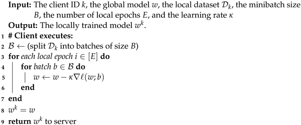
2.2. Federated Learning

The notion of FL is first proposed by McMahan et al. [21]. Algorithm 1 shows the well-known Federated Averaging (FedAvg) [21] protocol. Here we give a detailed interpretation. First, on line 2, the server assigns each client with the same initialized w 0 . In each communication round t, the server chooses a set of clients C t . Each client k C t in possession of a local dataset P k follows Algorithm 2 to train a local NN model w k , and uploads local model to the server. Next, on line 10, the server aggregates the uploaded client models of all clients in C t in the t-th communication round, to produce the global model w t for next communication round. The protocol then repeats, where the server re-distributes the model w t to clients for the next epoch of local training.
Algorithm 1: Federated Averaging.
Electronics 12 00842 i001
Algorithm 2: ClientUpdate ( k , w ) .
Electronics 12 00842 i002
   We note that most (if not all) traditional FL protocols distribute the same global model to each and every client. Consequently, Byzantine attack has become one of the most powerful attacks against FL systems.

2.3. Adversarial Attack

The notion of adversarial attack is first proposed by Goodfellow et al. [22], and is proven powerful against centralized learning mechanisms [23]. When the adversary is able to obtain full access to the victim model, the adversarial attack is known as white-box attack [24], which is the case for traditional FL systems in the presence of a corrupted client. Upon receiving the victim model f, the adversary begins to generate adversarial samples. The goal of the attack is to find some δ such that f ( x + δ ) f ( x ) . Here, the optimized x + δ is referred to as the adversarial samples.

2.4. Adversarial Training

Adversarial training [22] seeks to train deep neural networks that are robust against adversarial samples by leveraging robustness optimization. For each data point x D and its label y, adversarial training introduces a set of perturbations δ S . Let L denote the loss function (e.g., the Cross-Entropy loss). The objective function of adversarial training is as follows:
min f E ( x , y ) D max δ S L ( f , x + δ , y ) .
For the inner maximization of the saddle point formulation in Equation (1), the projected gradient descent (PGD) method [25] is usually applied. PGD adopts an iterative approach to generating the optimized adversarial sample x + δ from some clean sample x. In the iteration of PGD method, for each step t, it essentially executes projected gradient descent on the negative loss function
x t = Π x + S ( x t 1 + δ step sign ( Δ x L ( f , x , y ) ) ) .

3. Related Works

3.1. Federated Adversarial Training

Adversarial training is a typical method to enhance model robustness  [22,26,27,28,29,30,31]. Recently, many works explored the application of adversarial training in FL. Adversarial training is originally developed primarily for IID data, and it is still challenging to be carried out in non-IID FL settings. Zizzo et al. [32] took the first step towards federated adversarial training (FAT), and evaluated the feasibility of practical FAT in realistic scenarios. The main objective of FAT is to utilize adversarial training to solve the robustness and accuracy challenges faced by FL systems when applied in real-world tasks.

3.2. Byzantine-Robust Federated Learning

A stream of works have considered Byzantine-robust federated learning. Generally speaking, FL clients exchange knowledge through the aid of a trusted server. Under this setting, any client can be an adversary who wants to damage or poison the federated model. i.e., a Byzantine failure can occur within the FL system when clients become malicious. Byzantine-type attacks against FL systems include untargeted poisoning attacks [14,15,17,33] and targeted poisoning attacks [20].
To deal with Byzantine failures, several techniques are proposed to perform robust aggregation of user updates [34,35,36] or to detect and eliminate malicious user updates by similarity-based metrics [17,18,19,37]. Zizzo et al. [32] analyzed federated adversarial training in the presence of Byzantine clients, and concluded that it is still an open problem if both Byzantine-robustness and adversarial-robustness can co-exist within an FL system. Wang et al. [38] gave the theoretical proof that the existence of an adversarial sample implies the existence of a backdoor attack.

3.3. Research Gaps and Our Goal

Existing works on federated adversarial training try to train one globally robust model through the cooperation of all clients. If we adopt this traditional adversarial training procedure, the robustness of the global model will be indeed enhanced. Nonetheless, in the presence of a Byzantine failure (i.e., corrupted clients), successful adversarial samples generated on one client through powerful white-box attacks can still be perfectly transferred to other client models, rendering the entire system vulnerable. Therefore, we point out that none of the above works follow our definition of DMR, and are independent from our work. In defining DMR and instantiating an effective DMD technique, our main objective is to differentiate client models, so as to resist adversarial attack in the presence of a Byzantine failure.
In regard of Byzantine-robustness, we share the similar goal with Byzantine-robust federated learning, i.e., to develop Byzantine-robust federated learning frameworks. However, our key insight is that, if we distribute different models to different clients, we can significantly increase the difficulty of the corrupted clients to launch attacks. The challenge is how to maintain the overall model utility while carrying out the differentiating procedure.

4. Methodology

In this section, we first define a set of notions to assist us in formalizing the notion of DMR under FL. Then, we discuss the threat model we consider in this work. Next, we propose a concrete DMD method to improve the DMR of client models and introduce the ARMOR framework. Finally, we analyze the robustness for FL under DMD.

4.1. Definition

To formulate the differential robustness of our framework, we present two important metrics: Attack Success Rate (ASR) and Average Adversarial Transfer Rate (AATR). While ASR is a conventional metric to measure the attacking capability of an adversary, AATR is a novel metric that evaluates the transferability of adversarial samples within a multi-client FL system.
The definitions for ASR vary in different works [24,39,40,41,42]. In this work, we define ASR as follows. For any clean dataset D , D adv is the set of adversarial samples generated from D by some adversary A , i.e., for any d i A D adv , there exists some δ i such that d i A = d i + δ i , where d i D and | δ i | δ max . Under this setting, we define ASR as follows.
Definition 1
(Attack Success Rate). The adversary A chooses a clean dataset D , and generates the adversarial dataset D adv . For some victim model X, we denote the set of all d i D that X predicts correctly by D X , and the set of all corresponding d i A by D adv X . For each d i A D adv X , if X gives incorrect prediction on d i A , we call d i A a successful adversarial sample. Denote the set of all successful adversarial samples d i A by S adv X , and the set of all corresponding d i by S X . We say that the attack success rate of the adversary A on the victim model X is ASR D A , X = | S X | / | D X | .
ASR describes how effective is the attack launched by the adversary against a single victim model. In an FL scheme where clients receive different global models, however, we need a new metric to describing the transferability of adversarial samples across clients. We consider a K-client FL system with one malicious client the adversary A and K 1 benign clients. Under this setting, we define AATR as follows.
Definition 2
(Average Adversarial Transfer Rate). The adversary A first chooses a clean dataset D , and generate the adversarial dataset D adv from D . For each pair of d i D and d i A D adv , assume that a total number of i benign clients give correct predictions on d i but incorrect predictions on the corresponding d i A . Then, we say that the adversarial transfer rate of d i A is ATR d i A = i / ( K 1 ) . The average adversarial transfer rate is defined as AATR D adv A = E d i A D adv ( ATR d i A ) .
Note that in differentially robust FL, the malicious client has no knowledge of the exact parameters of other benign client models. As a result, A cannot decide which adversarial samples generated can be more powerful over the others. Thus, A can only use adversarial samples that are correctly classified on its own model to launch adversarial attacks against the benign clients.
With AATR in hand, we are ready to formalize the notion of Differential Model Robustness (DMR) in FL setting. We point out that there are two (somewhat conflicting) goals that the server wishes to achieve here. On the ond hand, the server wants the client models to stay close to the global model when predicting on the clean samples. On the other hand, client models should respond as different as possible against adversarial samples. Formally, we express the above idea of DMR as follows.
Definition 3
(Differential Model Robustness). Let I be the indicator function such that I ( F ( x ) ) = 1 if F ( x ) is the correct classification of sample x. Given an FL system with one malicious client, K 1 benign clients, and some generalization dataset G , let the global model be some function Y, and the differentiated client models be functions X j for j [ K 1 ] . We say that the system achieves ( ρ , ϵ , δ max ) -DMR if the following inequalities hold:
min j [ K 1 ] g i G I ( X j ( g i ) ) | G | g i G I ( Y ( g i ) ) | G | ρ ,
AATR D adv A ϵ .
Here, when A generates d i A = d i + δ i from d i , we restrict the amount of perturbations that the adversary A can add to the clean data samples by | δ i | δ max .
In Equation (3), the left hand side is the minimum accuracy of the differentiated client models, and the right hand side is the accuracy of the global model with an acceptable accuracy deterioration of ρ . In other words, Equation (3) expresses our utility demand inside the notion of DMR, where client models should respond similarly to the global model over clean samples. Meanwhile, Equation (4) gives the maximum level of AATR, which describes the robustness towards adversarial samples across different clients, i.e.,  how client models respond differently against adversarial samples.

4.2. Threat Model

We assume that the server and all clients participating in the the learning procedure of the original FL system are honest, which means that the server aggregates local models in the way it is supposed to, and each client honestly trains the local model using its own private dataset (we assume that any malicious local model update in the learning procedure can be detected or terminated by the server, since there exists various effective robust aggregation method [17,18,19,35,36,37]). However, after the global model being distributed to all clients, there exists one client that is malicious or compromised by a third-party adversary. As mentioned, we call this corrupted client the adversary A . In this work, the attack is outside of the pristine FL learning procedure, and is targeted at the model which will be deployed by each client to its practical applications.
Adversary’s capability. We consider a K-client federated learning system with one client is malicious or compromised by a third-party adversary, and other K 1 clients are benign. The adversary is assumed to have the following attack capabilities.
  • To access the local training data of the compromised client, but have no knowledge of the private training datasets of other benign clients.
  • To launch white-box attacks at its will, as any client participating in the training process of FL has direct access to its own local model parameters and the global model parameters.
Adversary’s goal. Different from a centralized learning scheme, the goal of an adversarial attack under a distributed learning setting is to find some perturbation δ such that other clients, as many as possible, classify the adversarial sample d adv = d + δ incorrectly. Formally, let I adv be the indicator function where I adv F , d ( y ) = 1 if y F ( d ) and 0 otherwise, and  X j be the differentiated model received by client j, the above idea can be expressed as the optimization over
arg max δ j = 1 L I adv X j , d X j ( d + δ ) ,
and that | δ | δ max to restrict the perturbation. However, we note that in practical FL systems, the number of benign clients can be very large, and according to Theorem 1, we can hardly achieve Equation (5) when there are enough number of benign clients whose models are properly differentiated. Therefore, we also define an empirical goal for the adversary in terms of the AATR simply as
arg max D adv AATR D adv A .

4.3. Intuitions and Framework Overview

In this section, we give the intuition and overview of our approach to enhancing DMR of FL systems. Then we propose the ARMOR framework as a concrete construction of our differential model distribution.
  • Targeted Problem: As described in Section 4.2, we consider adversarial attacks launched by Byzantine clients inside the FL systems. A Byzantine client has direct access to the global model and can construct effective adversarial samples efficiently. In traditional FL protocols, the server distributes the same global model to each client. Consequently, adversarial samples constructed by the Byzantine client can easily attack all of other benign clients. We aim at preventing such Byzantine adversarial attacks from generalizing inside the FL system.
  • General Solution: Our main insight is that model differentiation can reduce the transferability of adversarial samples among clients in FL systems. However, if we conduct trivial model differentiation, such as adding noise in the way similar to differential privacy, a satisfactory level of differential model robustness will be accompanied by high levels of utility deteriorations. We manage to attain the same level of utility over normal inputs while keeping the client models as different as possible against adversarial inputs. We discover that combining with suitable differentiating operations, adversarial training can be useful to produce differentially robust models.
As is illustrated in Figure 1, the ARMOR framework can be roughly divided into three parts: sub-federated model generating phase, adversarial sample generating phase and differential adversarial training phase. Here we give the intuitional explanation and general description of the three phases.
Phase 1. Sub-Federated Model Generating:
  • Intuition: In traditional FL systems, there is only one aggregated model known as global model (or federated model). If we develop our differential client models from the same global model, the differentiation can be too weak to powerful Byzantine clients. We try to find out how to decide the directions in which we differentiate the global model.
  • Solution: The last round of aggregation is shown in Algorithm 3. From Line 12 to 15, after getting all client model updates, for each client, the server randomly aggregates a set of client models into a sub-federated model. System manager can decide the number of clients included in one sub-federated model by adjusting the proportion parameter to achieve satisfactory model utility. That is, for a total of K clients, the server will generate K different sub-federated models for preparation of directing and regulating the subsequent differential adversary training phase.
Algorithm 3: Differential Model Distribution.
Electronics 12 00842 i003
Phase 2. Adversarial Samples Generating:
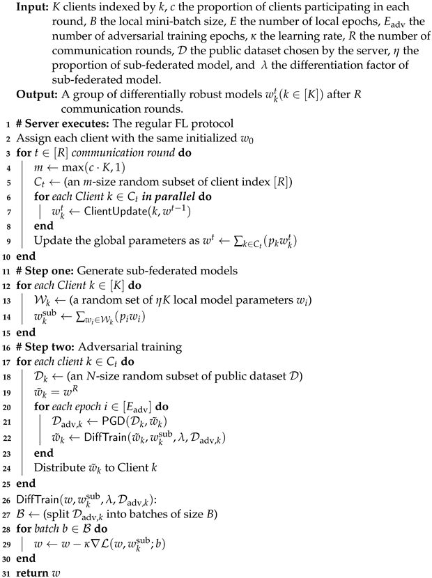
  • Intuition: In centralized adversary training, the server generates adversarial samples through adversarial attack methods such as FGSM attack [22] or PGD attack [25]. If we simply follow the same paradigm and utilize the whole public dataset to train the global model, we will come back to the problem of Byzantine clients again. As pointed out in Section 3.3, it is dangerous for all clients to hold the same global model in the model deployment phase. We need to generate different adversarial samples for each client.
  • Solution: As shown in Algorithm 3, from Line 17 to 21, after aggregating client models in the last round into a final global model, the server further generates adversarial samples based on the final global model. For each client, the server chooses a different set of samples from its public dataset, and uses different randomness to generate adversarial samples from the chosen sample set. That is, for a total of K clients, the server will generate K different sets of adversarial samples.
Phase 3. Differential Adversary Training:
  • Intuition: Now, we need to find an efficient way to conduct the differentiation while retaining the model accuracy. We are faced with two challenges. First, how to decide the metric of model distance (or model similarity)? A suitable metric is extremely important as it will directly influence our differential adversary training directions. Second, how to quantitatively produce different levels of differentiation? As model utility and DMR is a trade-off, a higher level of differentiation will lead to stronger DMR but weaker model utility. We should be able to adjust the level of differentiation to achieve a balance between utility and DMR.
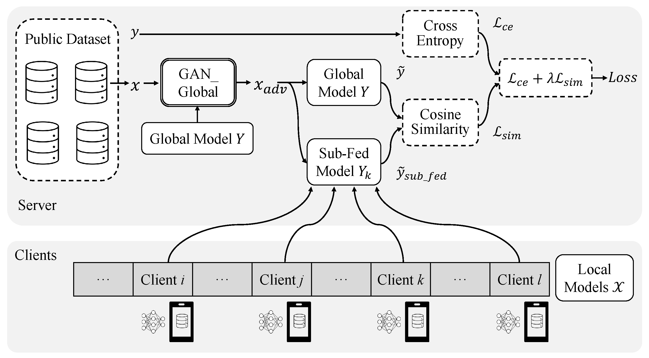
  • Solution: Utilizing Phase 1 and Phase 2, the server allocates each client a sub-federated model and a set of adversarial samples. When conducting differential adversarial training, we choose cosine similarity as the criterion to measure model distance. We use the cosine similarity between the output vectors of global model and sub-federated model to construct a similarity loss. We combine the similarity loss with the regular cross-entropy loss during adversarial training to accomplish our goal of differentiation.

4.4. Key Algorithms In ARMOR

As discussed in Section 4.3, in the ARMOR framework, our differential adversarial training consists of two types of differentiation followed by a differentiation fusion step. The detailed algorithm is given in Algorithm 3. Here, we give a line-by-line interpretation of Algorithm 3.
We consider an FL system with K clients. From Line 1 to 10, ARMOR follows the traditional FL protocol. We choose the standard Federated Averaging (FedAvg) [21] protocol as the basic FL algorithm. On Line 2, the server samples an initialized global model w 0 and assigns each client with the same initialized w 0 . We assume the total number of global communication rounds to be R. For each round t [ R ] , the server first computes the number of clients participating in this training round as m max ( c · K , 1 ) . Then the server randomly samples an m-size random subset of client index [ R ] . We denote the collection of these m clients by C t . Each client k in C t executes ClientUpdate to train the current global model w t 1 using its own local dataset, and outputs local model update w k t (The description of ClientUpdate is shown in Algorithm 2). When all clients in C t complete their local training and return the local model update, the server updates the global parameters as w t k C t ( p k w k t ) .
Then, Lines 11 to 25 describe what we refer to as the differential adversarial training technique, which is proven effective in enhancing the DMR while retaining a high level of utility of each client model. Differential adversarial training can be divided into two steps. In the first step, i.e., Line 11 to 15, the server generates sub-federated models for clients. The server first decides a factor η , which denotes the proportion of clients included in one sub-federated model. For each client k [ K ] , the server randomly samples a set of η K local model parameters w i , and aggregates them into sub-federated model for client k as w k sub w i W k ( p i w i ) . In the second step, i.e., Line 16 to 25, the server conducts adversarial training. We assume the total number of adversarial training epochs to be E adv . For each client k [ K ] , the server randomly samples an N-size subset of public dataset D . In each adversarial training epoch i [ E adv ] , the server uses PGD method to generate adversarial samples D adv , k , and executes DiffTrain to finish the training procedure. The DiffTrain algorithm is described in Line 26 to 30, which is run by the server to produce differentiated models based on the global model, the chosen sub-federated model and the chosen adversarial samples. Finally, for each client k [ K ] , the server distributes w ˜ k to client k.
The formal descriptions of the three key components in the ARMOR framework are given as follows.
  • Sub-Federated Model Based Model Differentiation: At the last round of aggregation, the server gets the set of all local models X = { X 1 , X 2 , , X K } from K clients, and aggregate these local models into a global federated model Y = X i X ( p i X i ) (With some abuse of notations, we use Y = X i X ( p i X i ) to denote the server’s operation of aggregating several local models X i with model parameter w i to generate the global model Y with model parameter w, i.e., w = i = 1 | X | p i w i . In this work, we have p i = 1 / | X i | , i [ | X | ] .). For each client k, the server randomly chooses η K local models from the set X to form a subset X k , and aggregate the η K local models in X k into a sub-federated model Y k = X i X k ( p i X i ) . We denote the set of all sub-federated models by Y sub = { Y 1 , Y 2 , , Y η K } .
  • Adversarial Samples Based Model Differentiation: In ARMOR, the server generates K different sets of adversarial samples based on the global model. For each client k, the server chooses a set of samples D k from its public training dataset D , and adopts PGD method [25] to generate a set of adversarial samples D adv , k in preparation for adversarial training. In this step, each adversarial dataset D adv , k for k [ K ] contains a different flavor of robustness, which will be introduced to the global model in the following adversarial training phase.
  • Differential Adversary Training: Combining the above two steps, the server associates each Client k with a sub-federated model Y k and a set of different adversarial samples D adv , k . Figure 2 illustrates the detailed relationships between models and losses in our training process. The server executes DiffTrain in Algorithm 3 to make each client find its way from Y towards the direction between Y k and the robustness introduced by D adv , k . Next, for DiffTrain , our goal is to produce differentiated model Y k based on the global model Y (we note that directly using Y k as the k-th client model results in degraded accuracy performance). Here, we choose the cosine distance as the criterion to measure the similarity between the global model and the sub-federated models. Given input samples D adv , k , we compute the cosine embedding loss of the output of global model Y and the corresponding sub-federated model Y k . Let Y and Y k be the model functions whose outputs are the probability vectors over the class labels. We define the similarity loss for sample d i A as
    sim , i ( Y , Y k ) = 1 Y ( d i A ) · Y k ( d i A ) T Y ( d i A ) 2 × Y i ( d i A ) 2 ,
    where · is the inner product between vectors, · 2 depicts the L 2 -norm of a vector, and × denotes integer multiplication. When measuring similarity, we define the target labels T = { t 1 , t 2 , , t | D adv , k | } for the cosine similarity loss, where each t i follows the Bernoulli distribution P ( t i ) where Pr [ t i = 1 ] = p . Then, we use T to select a portion of p samples with label 1 to participate in similarity measurement. Now, we have our total cosine similarity loss
    L sim ( Y , Y k ) = d i A D adv , k t i × sim , i ( Y , Y k ) | D adv , k | .
In addition to the similarity measurement, we follow the method of [22] to train on a mixture of clean and adversarial examples. We compute the regular cross-entropy loss L ce between input D adv , k and the label set of the corresponding clean dataset D k as
L ce ( Y ) = d i A D adv , k ce , i ( Y , d i ) + ce , i ( Y , d i A ) × 1 | D adv , k | .
Combining the two losses, we have our final objective loss function as
L = L ce ( Y ) + λ L sim ( Y , Y k ) ,
where λ is the controlling factor to decide how strong our differential models will be differentiated in the directions of the randomly generated sub-federated models.

4.5. Robustness Analysis

Before delving into the theory, we first note that there exists adversarial perturbations which are effective against any classifier [43,44,45]. As a result, when only a small number (e.g., one) client is benign in an FL system, the derivations in [43] indicate that there is an upper limit on the adversarial robustness of any classifier.
Consequently, we seek the following alternative. From a high level of view, the differential model distribution technique, i.e., the differential adversarial training method we proposed above, can be seen as conducting stochastic perturbations to the global model while retaining an acceptable level of accuracy deterioration. Due to the randomness introduced by stochastic functions during the training procedure, we can take these perturbations as independent random variables added to the global model. Subsequently, the following theorem can be established.
Theorem 1.
We consider an K-client FL system with one malicious client and K 1 benign clients. Each client receives a linear classifier F i for i [ K ] . Assume that there exists some DMD mechanism in the FL system such that for any two benign client models F i ( x ) = w i x and F j ( x ) = w j x where i j , it holds that w i = w + β i and w j = w + β j where β i and β j are independent random variables satisfying β i , β j β min for all i , j [ L ] . Then, for any adversarial sample d i A = d i + δ i with restriction of | δ i | δ max , we have that
Pr [ ATR d i A θ ] ( 1 γ ) θ ( K 1 )
for some real numbers θ , γ [ 0 , 1 ] .
Proof. 
We can prove the theorem via a simple probabilistic argument. Without loss of generality, we assume that the malicious client is Client 0. First, observe that for any successful adversarial sample d A = d + δ on the corrupted client, it holds that
sign ( w 0 ( d + δ ) ) sign ( w 0 ( d ) ) .
Expanding the terms, we get
sign ( w 0 d + w 0 δ ) sign ( w 0 d ) , which means that
sign ( w d + β 0 d + w δ + β 0 δ ) sign ( w d + β 0 d ) .
For the adversarial sample d A to transfer to the j-th client, we need to achieve a similar goal, i.e.,
sign ( w d + β j d + w δ + β j δ ) sign ( w d + β j d ) .
Since both Client 0 and Client j correctly classify d (which is a necessary condition for any adversarial attack to be meaningful), we know that
sign ( w d + β j d ) = sign ( w d + β 0 d ) .
Then, we know that the objective of transferring the adversarial sample from Client 0 to the Client j can be formulated as
sign ( w d + β j d + w δ + β j δ ) = sign ( w 0 ( d + δ ) ) .
We point out that w j can be formulated as a “differentiated” version of w 0 , i.e.,
w j = w 0 + β 0 j ,
where β 0 j = β 0 + β j . As a result, the LHS for Equation (17) becomes
sign ( w 0 ( d + δ ) + β 0 j ( d + δ ) ) = sign ( w 0 ( d + δ ) ) .
Here, we can consider the term β 0 j ( d + δ ) as an additive noise to the classification result w 0 ( d + δ ) , which is a label that is the opposite of w 0 d . Now, to satisfy the objective of Equation (17), we basically need the noise of β 0 j ( d + δ ) to be small enough such that the addition of this term does not cause the classification result to cross the decision boundary (i.e., flip the sign). Unfortunately, from the results in [43], we know that the robustness of any classifier is bounded from above. Let ξ denote that the probability of classifying the result to 1, then the probability of 0 becomes 1 ξ , and the fraction of adversarial samples that does not work on w j becomes
Pr ( R ( x ) η ) 1 π 2 e ω 1 ( η ) 2 / 2 ,
where R ( x ) = min δ | | δ | | such that w 0 ( x + δ ) w 0 ( x ) (i.e,. the robustness of the input sample x), η is the robustness threshold, ω is the modulus of continuity, Simialr to [43], when we take ω 1 ( η ) = η / L where L is the Lipschitz constant, we have that
Pr ( R ( x ) η ) 1 π 2 e ( η / L ) 2 / 2 .
Replacing x with the adversarial sample d + δ , we see that the stability of transferring the adversarial sample can be seen as its robustness, and this robustness is bounded from above by some factor η . Hence, when we have a model-wise perturbation that is larger than the robustness of the adversarial sample, i.e.,
β 0 j ( d + δ ) η ,
the j-th model will produce a “mis-classified” adversarial sample with non-negligible probability, which is exactly the probability of the j-th model to produce a correct prediction on the adversarial sample in the binary classification case. Since β 0 j can be adjusted according to β max , we are guaranteed that
Pr [ sign ( w 0 ( d + δ ) + β 0 j ( d + δ ) ) = sign ( w 0 ( d + δ ) ) ]
= Pr [ sign ( w 0 ( d + δ ) + η ) = sign ( w 0 ( d + δ ) ) ]
= 1 Pr [ R ( x ) η ]
1 Pr [ R ( x ) β 0 j ( d + δ ) ] .
Let γ = Pr [ R ( x ) β 0 j ( d + δ ) ] , we then know that the probability that any adversarial sample d + δ can transfer to the j-th client model is 1 γ . Since all pairs of β 0 j for j [ K 1 ] is mutually independent, the probability that an adversarial sample d A simultaneously transfers to benign clients is ( 1 γ ) . Then, we have that for any adversarial sample d A ,
Pr [ All clients are compromised ] = ( 1 γ ) .
As defined in Definition 2, since is the number of clients that are compromised, ATR d A = / ( K 1 ) , we have
Pr [ ATR d A θ ] = Pr [ / ( K 1 ) θ ] ( 1 γ ) θ ( K 1 ) ,
and the theorem follows. □
We note that Equation (28) goes to a probability of 0 as the total number of benign clients K 1 goes to infinity. That is to say that, for any adversarial sample d A and any attack transfer rate θ that is non-zero, the probability of an adversary achieving this ATR goes to zero when the number of benign clients grow.

5. Experiment Results

5.1. Experiment Flow and Setup

To validate the effectiveness of our DMD method, we perform experiments in FL settings of different client numbers, and in each setting we balanced the partition of the whole training dataset among all clients in a non-i.i.d. manner. We follow the DMD technique described in Algorithm 3 to conduct our experiment. In this experiment, we take nine different FL settings of clients number K = 10 , 15 , 20 , 25 , 30 , 35 , 40 , 45 , 50 and set c = 1 in FedAvg algorithm.
  • Physical Specifications: We conduct our experiments on Linux platform with NVIDIA A100 SXM4 with a GPU memory of 40GB. The platform is equipped with a driver of version 470.57.02 and CUDA of version 11.4.
  • Datasets: We empirically evaluate the ARMOR framework on two datasets: MNIST [46] and CIFAR-10 [47]. To simulate the heterogeneous data distributions, we make non-i.i.d. partitions of the datasets, which is a similar partition method as [21].
    (1)
    Non-IID MNIST: The MNIST dataset contains 60,000 training images and 10,000 testing images of 10 classes. Each sample is a 28 × 28 size gray-level image of a handwritten digit. We first sort the training dataset by digit label, divide it into 3 K shards of size 60 , 000 / K , and assign each client 3 shards.
    (2)
    Non-IID CIFAR-10: The CIFAR-10 dataset contains 50,000 training images and 10,000 test images of 10 classes. Each sample is a 32 × 32 size tiny color image. We first sort the training dataset by class label, divide it into 4 K shards of size 50 , 000 / K , and assign each client 4 shards.
  • Model: For the MNIST dataset, we use a CNN model with two 5 × 5 convolution layers (the first with 4 channels, the second with 10 channels, each followed with 2 × 2 max pooling), a fully connected layer with 100 units, an ReLu activation, and a final output layer. For the CIFAR-10 dataset, we use the VGG-16 model [48].
  • Hyperparameters: For both datasets, we first train with the federated averaging algorithm. In each communication round, we let all clients to participate in the training (i.e., c = 1 ), where the client model is trained by one epoch using the local datasets. On the server side, the model update from each client is weighted uniformly (since we assume that each client has the same number of training samples). For MNIST and CIFAR-10, we set the number of communication round R to 50 and 500, the learning rate κ to 0.07 and 0.05 , and the client batch size to 10 and 64, respectively.
When applying the PGD attack for adversarial training, we need to decide the upper bound on the gradient steps in the -norm. For MNIST, the server uses 1000 public images to generate adversarial samples for training, each adversarial sample is constructed with δ max = 0.2 (also denoted as ε in many works) as the max perturbation range by a step size of δ step = 0.01 for 40 iterations, while for CIFAR-10, we choose 1000 public images with δ max = 0.03 by a step size of δ step = 0.008 for 20 iterations. Note that we have K clients in this FL setting, so the server generates K different sets of adversarial samples based on the global model.

5.2. Main Results

In this section, we show the results of applying ARMOR over the MNIST and CIFAR-10 datasets.

5.2.1. Results on MNIST

Table 1 illustrates the results of the average model accuracy over all clients, and average ASR and AATR of adversarial samples on benign clients with a varying number of FL clients. Before delving into the results, we first explain the subtle relationship between Acc and Acc D . Recall that our goal is to make the client models stay close to the global model when predicting the clean samples while responding as differently as possible against adversarial samples. Here, Acc is the accuracy on randomly selected testing samples, while Acc D is the accuracy on clean dataset D . Note that when launching attacks, A only chooses successful adversarial samples (i.e., misclassified by the client model of A ) whose clean samples can be correctly classified using its own client model. In other words, for the client model of A , ASR D A = 100 % . Therefore, the difference between Acc and Acc D indicates whether correctly predicted samples in D is different from the datasets of all other clients. To this end, Table 1 confirms that Acc D is almost identical to Acc . The conclusion here is that, the adversary A cannot tell which sample will be more susceptible to the other models possessed by the benign clients with high confidence.
Comparing the accuracy and AATR of models with and without our differential adversarial training, we point out that model utility and DMR is indeed a trade-off. For example, for client number K = 35 in Table 1, after deploying our DMD technique, we are able to reduce the ASR on benign clients from 100% to 15.21% and AATR from 100% to 20.45% while maintaining the overall client model accuracy of 90.35%. At the same time, as the number of FL clients increases, AATR in Table 1 exhibits a smooth decrease, as predicted in Section 4.5.
We present the frequency of the average transfer rate of each adversarial sample generated by adversary A in Figure 3. Note that without our DMD method, the ATR of every adversarial sample is 100 % , and consequently, the AATR is also 100 % . Here we have the following two main remarks.
Remark 1.
The empirical observations agree with Theorem 1. Due to this special property, apart from our differential adversarial training method, we can develop more DMD techniques to step further towards the DMR goal in FL and propose various trustworthy FL protocols under the presence of Byzantine failure.
Remark 2.
The DMR improvement due to the proposed DMD technique increases when the client number K of FL increases. Intuitively, as the number of FL clients increases from 10 to 30, the distribution histograms are pushed toward the zero-ATR side, and the shape becomes more squeezed and narrow. This trend shows that as the client number increases, the sub-federated models become more different from each other, which makes the differentially distributed client models more robust against attacks from the malicious FL client.
By applying differential adversarial training to the global model, we are able to control the attack transferability within an acceptable range. For example, we consider the FL setting of K = 40 clients in Figure 3c. With our differential adversarial training method, we obtain an AATR of 19.47 % . With this level of AATR, we can make sure that 45% of the adversarial samples generated by the malicious client have ATR 10 % , while 75% samples have that ATR 30 % . In particular, almost no adversarial samples can achieve an ATR of 100 % .

5.2.2. Results on CIFAR-10

Similar to the analyses for MNIST, as is illustrated in Table 2, ARMOR can reduce ASR and AATR of benign clients over the CIFAR-10 dataset as well. For example, for K = 35 , if we apply the DMD method, the ASR is reduced from 100% to 26.09% and the AATR can be reduced from 100% to 35.07%. Results on both datasets confirm that ARMOR is effective in reducing the vulnerability of FL client models against Byzantine-style adversarial attacks.
Comparing Table 2 with Table 1, we can find that accuracy deterioration in Table 2 is much higher than that in Table 1. If we keep accuracy deterioration in Table 2 around the same level of Table 1, the reduction of ASR and AATR on CIFAR-10 will be less than that on MNIST. As a potential explanation, existing works [25,27,49] show that, under a centralized learning setting, various adversarial training methods are generally less effective on models trained on CIFAR-10 than models trained on MNIST. For example, in centralized settings [25], PGD adversarial training achieves a robustness of at most 45.80% (ASR = 54.20%) in CIFAR-10 while achieving a much better robustness of 89.30% (ASR = 10.70%) in MNIST.

5.3. Ablation Study

Differentiation methods: In Table 3, we perform the ablation studies on our framework over the MNIST dataset to confirm that both of the sub-federated model-based and adversarial sample-based differentiation techniques are crucial in improving the DMR of FL. We note that, in the case where we directly perform adversarial sample based differentiation without sub-federated model generation, the objective function is reduced to the cross-entropy loss
L ce ( Y ) = d i A D adv , k ce , i ( Y , d i ) + ce , i ( Y , d i A ) × 1 | D adv , k | .
Comparing the trends of ASR and AATR as the DMD method and client number K changes, we have two main observations here:
  • First, the adversarial samples based model differentiation does have a positive influence on reducing ASR and AATR of benign clients. Nevertheless, the reduction is limited. However, when combined with the sub-federated model-based model differentiation, both ASR and AATR of benign clients are reduced significantly. For example, when K = 50 , if we only apply L ce based DMD, the AATR is reduced from 100% to 52.29%. If we further combine L ce with L sim , the AATR is further reduced to 23.17%, which demonstrates that the key in enhancing DMR is the combination of sub-federated model generation and differential adversarial training.
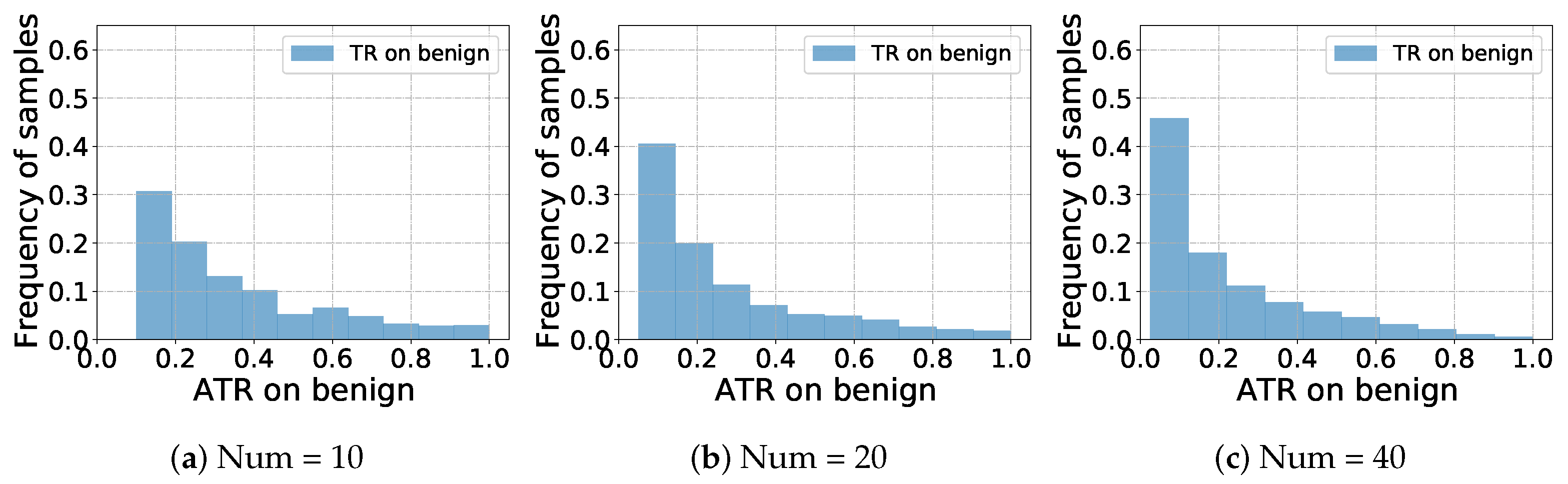
  • Second, the DMR improvement increases as the client number K of FL increases. Table 4 illustrates that ASR and AATR decrease as K increases. For example, when applying L ce + λ L sim , the AATR is 40.89% for 10 clients, 26.54% for 25 clients, and 23.17% for 50 clients. This is reasonable because as the client number increases, the diversity of sub-federated model is enlarged. As sub-federated models become more different from each other, the differentially distributed client models become more robust against attacks from the malicious client, resulting in additional DMR improvements.
The impact of DMD parameters: As is shown in Table 4, we choose five different combinations of the proportion of sub-federated model η , the differentiation factor of sub-federated model λ and the probability p of Bernoulli distribution: (1) λ = 500 , η = 0.25 , p = 0.10 , (2) λ = 600 , η = 0.25 , p = 0.10 , (3) λ = 600 , η = 0.35 , p = 0.10 , (4) λ = 300 , η = 0.25 , p = 0.20 , (5) λ = 350 , η = 0.25 , p = 0.20 . When the differentiation factor λ increases, clients’ models tend to produce more mispredictions. Hence, the server needs to carefully adjust λ to retain a practical level of utility while improving the robustness for the differentiated client models. Comparing the results of different DMD parameters settings, we have two main observations here:
  • First, the DMR of FL client models is strengthened as the differentiation factor λ increases. We fix η = 0.25 and p = 0.10 , then set λ = 500 and λ = 600 , respectively. Similarly, we fix η = 0.25 and p = 0.20 , then set λ = 300 and λ = 350 , respectively. We find that for p = 0.10 (resp., p = 0.20 ), DMD with λ = 600 (resp., λ = 350 ) constantly leads to lower ASR and AATR than DMD with λ = 500 (resp., λ = 300 ), which validates the positive effect of the sub-federated model differentiation.
  • Second, we observe that as the proportion of sub-federated model η increases from 1 / K , the overall accuracy of model also increases. However, as long as the sub-federated model is of enough utility, further increasing η does not help much. We fix λ = 600 and p = 0.10 , then set η = 0.25 and η = 0.35 , respectively. We find that slight change in η does not lead to much differences in ASR and AATR. However, choosing only one single local model as the sub-federated model (i.e., η = 1 / K ) leads to significant deterioration of performance.
From the ablation study results, we conclude that the combination of sub-federated model based differentiation and adversarial sample based differentiation is effective in reducing both the ASR and AATR while maintaining the overall accuracy of the benign client models.

6. Discussion

We aim at ensuring the safety of FL systems when Byzantine failure occurs in real-life applications. Such failure is very likely to occur in real-world FL systems, and can be life-threatening when critical inference devices are attacked. For example, in the joint training of autonomous driving systems, each autonomous vehicle is deployed with an NN model under an FL setting. If there exists a malicious client in this system, the malicious client can easily generate adversarial samples to attack all other vehicles, potentially causing serious accidents. Consequently, all other vehicles in the system using the same model will collectively produce wrong predictions on these adversarial traffic signs, potentially causing serious accidents. ARMOR is one of the first works to explore defense mechanisms against such attacks, and can be essential in developing safe and trustworthy FL protocols.

7. Conclusions

In this work, we study the differential robustness of NN models against adversarial attacks in FL systems in the presence of Byzantine failures. By providing with clients carefully differentiated NN models, the main objective of the proposed ARMOR framework is to reduce the risks of corrupted FL clients launching white-box adversarial attacks against benign clients. By carefully designing the experiments and ablation studies under various FL settings, we show that techniques proposed in the ARMOR framework are indeed effective in reducing both the ASR and AATR of adversarial samples generated by the corrupted clients.

Author Contributions

Conceptualization, Y.Z., J.L., Z.G., X.L. and S.B.; methodology, Y.Z., S.B. and X.L.; software, Y.Z.; investigation, B.Z.; writing—original draft preparation, Y.Z. and B.Z.; writing—review and editing, Y.Z., S.B., J.L., Z.G., X.L. and B.Z.; supervision, J.L., Z.G., X.L. and S.B. All authors have read and agreed to the published version of the manuscript.

Funding

This work was supported in part by the National Key R&D Program of China under Grants 2021YFB2700200, in part by the National Natural Science Foundation of China under Grant 62202028, U21B2021, 61972018, and 61932014. This work was supported in part by PowerTensors.AI.

Institutional Review Board Statement

Not applicable.

Informed Consent Statement

Not applicable.

Data Availability Statement

A proof-of-concept implementation of our technique is available from https://github.com/ARMOR-FL/ARMOR (accessed on 19 December 2022). The data used to support the findings of this study are included within the article.

Acknowledgments

Our deepest gratitude goes to the anonymous reviewers for their careful work.

Conflicts of Interest

The authors declare no conflict of interest.

References

  1. Bonawitz, K.A.; Eichner, H.; Grieskamp, W.; Huba, D.; Ingerman, A.; Ivanov, V.; Kiddon, C.; Konečný, J.; Mazzocchi, S.; McMahan, B.; et al. Towards Federated Learning at Scale: System Design. In Proceedings of the Machine Learning and Systems 1 (MLSys 2019), Stanford, CA, USA, 31 March–2 April 2019. [Google Scholar]
  2. Li, T.; Sahu, A.K.; Talwalkar, A.; Smith, V. Federated Learning: Challenges, Methods, and Future Directions. IEEE Signal Process. Mag. 2020, 37, 50–60. [Google Scholar] [CrossRef]
  3. Long, G.; Tan, Y.; Jiang, J.; Zhang, C. Federated Learning for Open Banking. In Federated Learning—Privacy and Incentive; Lecture Notes in Computer Science; Springer: Berlin, Germany, 2020; Volume 12500, pp. 240–254. [Google Scholar]
  4. Guo, P.; Wang, P.; Zhou, J.; Jiang, S.; Patel, V.M. Multi-Institutional Collaborations for Improving Deep Learning-Based Magnetic Resonance Image Reconstruction Using Federated Learning. In Proceedings of the Conference on Computer Vision and Pattern Recognition (CVPR) 2021, Nashville, TN, USA, 20–25 June 2021; pp. 2423–2432. [Google Scholar]
  5. Du, Z.; Wu, C.; Yoshinaga, T.; Yau, K.A.; Ji, Y.; Li, J. Federated Learning for Vehicular Internet of Things: Recent Advances and Open Issues. IEEE Open J. Comput. Soc. 2020, 1, 45–61. [Google Scholar] [CrossRef] [PubMed]
  6. Pokhrel, S.R.; Choi, J. Federated Learning With Blockchain for Autonomous Vehicles: Analysis and Design Challenges. IEEE Trans. Commun. 2020, 68, 4734–4746. [Google Scholar] [CrossRef]
  7. Li, Q.; He, B.; Song, D. Model-Contrastive Federated Learning. In Proceedings of the Conference on Computer Vision and Pattern Recognition (CVPR) 2021, Nashville, TN, USA, 20–25 June 2021; pp. 10713–10722. [Google Scholar]
  8. Lai, F.; Zhu, X.; Madhyastha, H.V.; Chowdhury, M. Oort: Efficient Federated Learning via Guided Participant Selection. In Proceedings of the Operating Systems Design and Implementation (OSDI) 2021, Virtual, 14–16 July 2021; pp. 19–35. [Google Scholar]
  9. Zhang, C.; Li, S.; Xia, J.; Wang, W.; Yan, F.; Liu, Y. BatchCrypt: Efficient Homomorphic Encryption for Cross-Silo Federated Learning. In Proceedings of the USENIX Security 2020, San Diego, CA, USA, 12–14 August 2020; pp. 493–506. [Google Scholar]
  10. Wei, K.; Li, J.; Ding, M.; Ma, C.; Yang, H.H.; Farokhi, F.; Jin, S.; Quek, T.Q.S.; Poor, H.V. Federated Learning With Differential Privacy: Algorithms and Performance Analysis. IEEE Trans. Inf. Forensics Secur. 2020, 15, 3454–3469. [Google Scholar] [CrossRef]
  11. Shokri, R.; Stronati, M.; Song, C.; Shmatikov, V. Membership Inference Attacks Against Machine Learning Models. In Proceedings of the SP 2017, San Jose, CA, USA, 22–26 May 2017; pp. 3–18. [Google Scholar]
  12. Nasr, M.; Shokri, R.; Houmansadr, A. Comprehensive Privacy Analysis of Deep Learning: Passive and Active White-box Inference Attacks against Centralized and Federated Learning. In Proceedings of the SP 2019, San Francisco, CA, USA, 19–23 May 2019; pp. 739–753. [Google Scholar]
  13. Zhang, Y.; Jia, R.; Pei, H.; Wang, W.; Li, B.; Song, D. The Secret Revealer: Generative Model-Inversion Attacks Against Deep Neural Networks. In Proceedings of the Conference on Computer Vision and Pattern Recognition (CVPR) 2020, Seattle, WA, USA, 13–19 June 2020; pp. 250–258. [Google Scholar]
  14. Fang, M.; Cao, X.; Jia, J.; Gong, N.Z. Local Model Poisoning Attacks to Byzantine-Robust Federated Learning. In Proceedings of the USENIX Security 2020, San Diego, CA, USA, 12–14 August 2020; pp. 1605–1622. [Google Scholar]
  15. Shejwalkar, V.; Houmansadr, A. Manipulating the Byzantine: Optimizing Model Poisoning Attacks and Defenses for Federated Learning. In Proceedings of the Network and Distributed System Security Symposium (NDSS) 2021, Virtual, 21–25 February 2021. [Google Scholar]
  16. Kido, H.; Yanagisawa, Y.; Satoh, T. Protection of Location Privacy using Dummies for Location-based Services. In Proceedings of the International Conference on Data Engineering (ICDE) 2005, Tokyo, Japan, 3–4 April 2005; p. 1248. [Google Scholar]
  17. Blanchard, P.; Mhamdi, E.M.E.; Guerraoui, R.; Stainer, J. Machine Learning with Adversaries: Byzantine Tolerant Gradient Descent. In Proceedings of the NeurIPS 2017, Long Beach, CA, USA, 4–9 December 2017; pp. 119–129. [Google Scholar]
  18. Yin, D.; Chen, Y.; Ramchandran, K.; Bartlett, P.L. Byzantine-Robust Distributed Learning: Towards Optimal Statistical Rates. In Proceedings of the International Conference on Machine Learning (ICML) 2018, Stockholm, Sweden, 10–15 July 2018; pp. 5636–5645. [Google Scholar]
  19. Pillutla, K.; Kakade, S.M.; Harchaoui, Z. Robust aggregation for federated learning. IEEE Trans. Signal Process. 2022, 70, 1142–1154. [Google Scholar] [CrossRef]
  20. Bagdasaryan, E.; Veit, A.; Hua, Y.; Estrin, D.; Shmatikov, V. How To Backdoor Federated Learning. In Proceedings of the AISTATS 2020, Palermo, Italy, 26–28 August 2020; Volume 108, pp. 2938–2948. [Google Scholar]
  21. McMahan, B.; Moore, E.; Ramage, D.; Hampson, S.; y Arcas, B.A. Communication-Efficient Learning of Deep Networks from Decentralized Data. In Proceedings of the AISTATS 2017, Fort Lauderdale, FL, USA, 20–22 April 2017; Volume 54, pp. 1273–1282. [Google Scholar]
  22. Goodfellow, I.J.; Shlens, J.; Szegedy, C. Explaining and Harnessing Adversarial Examples. In Proceedings of the International Conference on Learning Representations (ICLR) 2015, San Diego, CA, USA, 7–9 May 2015. [Google Scholar]
  23. Szegedy, C.; Zaremba, W.; Sutskever, I.; Bruna, J.; Erhan, D.; Goodfellow, I.J.; Fergus, R. Intriguing properties of neural networks. In Proceedings of the International Conference on Learning Representations (ICLR) 2014, Banff, AB, Canada, 14–16 April 2014. [Google Scholar]
  24. Ru, B.; Cobb, A.D.; Blaas, A.; Gal, Y. BayesOpt Adversarial Attack. In Proceedings of the International Conference on Learning Representations (ICLR) 2020, Addis Ababa, Ethiopia, 26–30 April 2020. [Google Scholar]
  25. Madry, A.; Makelov, A.; Schmidt, L.; Tsipras, D.; Vladu, A. Towards Deep Learning Models Resistant to Adversarial Attacks. In Proceedings of the ICLR 2018, Vancouver, BC, Canada, 30 April–3 May 2018. [Google Scholar]
  26. Miyato, T.; Dai, A.M.; Goodfellow, I.J. Adversarial Training Methods for Semi-Supervised Text Classification. In Proceedings of the International Conference on Learning Representations (ICLR) 2017, Toulon, France, 24–26 April 2017. [Google Scholar]
  27. Shafahi, A.; Najibi, M.; Ghiasi, A.; Xu, Z.; Dickerson, J.P.; Studer, C.; Davis, L.S.; Taylor, G.; Goldstein, T. Adversarial training for free! In Proceedings of the NeurIPS 2019, Vancouver, CA, Canada, 8–14 December 2019; pp. 3353–3364. [Google Scholar]
  28. Zhang, D.; Zhang, T.; Lu, Y.; Zhu, Z.; Dong, B. You Only Propagate Once: Accelerating Adversarial Training via Maximal Principle. In Proceedings of the NeurIPS 2019, Vancouver, CA, Canada, 8–14 December 2019; pp. 227–238. [Google Scholar]
  29. Zhu, C.; Cheng, Y.; Gan, Z.; Sun, S.; Goldstein, T.; Liu, J. FreeLB: Enhanced Adversarial Training for Natural Language Understanding. In Proceedings of the International Conference on Learning Representations (ICLR) 2020, Addis Ababa, Ethiopia, 26–30 April 2020. [Google Scholar]
  30. Jiang, H.; He, P.; Chen, W.; Liu, X.; Gao, J.; Zhao, T. SMART: Robust and Efficient Fine-Tuning for Pre-trained Natural Language Models through Principled Regularized Optimization. In Proceedings of the ACL 2020, Virtual, 5–10 July 2020; pp. 2177–2190. [Google Scholar]
  31. Qin, C.; Martens, J.; Gowal, S.; Krishnan, D.; Dvijotham, K.; Fawzi, A.; De, S.; Stanforth, R.; Kohli, P. Adversarial Robustness through Local Linearization. In Proceedings of the NeurIPS 2019, Vancouver, CA, Canada, 8–14 December 2019; pp. 13824–13833. [Google Scholar]
  32. Zizzo, G.; Rawat, A.; Sinn, M.; Buesser, B. FAT: Federated Adversarial Training. arXiv 2020, arXiv:2012.01791. [Google Scholar]
  33. Bhagoji, A.N.; Chakraborty, S.; Mittal, P.; Calo, S.B. Analyzing Federated Learning through an Adversarial Lens. In Proceedings of the ICML 2019, Long Beach, CA, USA, 9–15 June 2019; Volume 97, pp. 634–643. [Google Scholar]
  34. Li, L.; Xu, W.; Chen, T.; Giannakis, G.B.; Ling, Q. RSA: Byzantine-Robust Stochastic Aggregation Methods for Distributed Learning from Heterogeneous Datasets. In Proceedings of the AAAI 2019, Honolulu, HI, USA, 27 January–1 February 2019; pp. 1544–1551. [Google Scholar]
  35. Kerkouche, R.; Ács, G.; Castelluccia, C. Federated Learning in Adversarial Settings. arXiv 2020, arXiv:2010.07808. [Google Scholar]
  36. Fu, S.; Xie, C.; Li, B.; Chen, Q. Attack-Resistant Federated Learning with Residual-based Reweighting. arXiv 2019, arXiv:1912.11464. [Google Scholar]
  37. Chen, Y.; Su, L.; Xu, J. Distributed Statistical Machine Learning in Adversarial Settings: Byzantine Gradient Descent. Proc. ACM Meas. Anal. Comput. Syst. 2017, 1, 44:1–44:25. [Google Scholar] [CrossRef]
  38. Wang, H.; Sreenivasan, K.; Rajput, S.; Vishwakarma, H.; Agarwal, S.; Sohn, J.; Lee, K.; Papailiopoulos, D.S. Attack of the Tails: Yes, You Really Can Backdoor Federated Learning. In Proceedings of the NeurIPS 2020, Virtual, 6–12 December 2020. [Google Scholar]
  39. Zhou, M.; Wu, J.; Liu, Y.; Liu, S.; Zhu, C. DaST: Data-Free Substitute Training for Adversarial Attacks. In Proceedings of the Conference on Computer Vision and Pattern Recognition (CVPR) 2020, Seattle, WA, USA, 13–19 June 2020; pp. 231–240. [Google Scholar]
  40. Wang, W.; Yin, B.; Yao, T.; Zhang, L.; Fu, Y.; Ding, S.; Li, J.; Huang, F.; Xue, X. Delving into Data: Effectively Substitute Training for Black-box Attack. In Proceedings of the Conference on Computer Vision and Pattern Recognition (CVPR) 2021, Nashville, TN, USA, 20–25 June 2021; pp. 4761–4770. [Google Scholar]
  41. Ma, C.; Chen, L.; Yong, J. Simulating Unknown Target Models for Query-Efficient Black-Box Attacks. In Proceedings of the Conference on Computer Vision and Pattern Recognition (CVPR) 2021, Nashville, TN, USA, 20–25 June 2021; pp. 11835–11844. [Google Scholar]
  42. Li, X.; Li, J.; Chen, Y.; Ye, S.; He, Y.; Wang, S.; Su, H.; Xue, H. QAIR: Practical Query-Efficient Black-Box Attacks for Image Retrieval. In Proceedings of the Conference on Computer Vision and Pattern Recognition (CVPR) 2021, Nashville, TN, USA, 20–25 June 2021; pp. 3330–3339. [Google Scholar]
  43. Fawzi, A.; Fawzi, H.; Fawzi, O. Adversarial vulnerability for any classifier. In Proceedings of the NeurIPS 2018, Montreal, QC, Canada, 3–8 December 2018; pp. 1186–1195. [Google Scholar]
  44. Tramèr, F.; Papernot, N.; Goodfellow, I.J.; Boneh, D.; McDaniel, P.D. The Space of Transferable Adversarial Examples. arXiv 2017, arXiv:1704.03453. [Google Scholar]
  45. Fawzi, A.; Fawzi, O.; Frossard, P. Analysis of classifiers’ robustness to adversarial perturbations. Mach. Learn. 2018, 107, 481–508. [Google Scholar] [CrossRef]
  46. LeCun, Y.; Cortes, C.; Burges, C.J.C. The MNIST Database of Handwritten Digits. 1998. Available online: http://yann.lecun.com/exdb/mnist/ (accessed on 20 January 2022).
  47. Krizhevsky, A. Learning Multiple Layers of Features from Tiny Images; University of Toronto: Toronto, ON, Canada, 2009. [Google Scholar]
  48. Simonyan, K.; Zisserman, A. Very Deep Convolutional Networks for Large-Scale Image Recognition. In Proceedings of the International Conference on Learning Representations (ICLR) 2015, San Diego, CA, USA, 7–9 May 2015. [Google Scholar]
  49. Wong, E.; Rice, L.; Kolter, J.Z. Fast is better than free: Revisiting adversarial training. In Proceedings of the International Conference on Learning Representations (ICLR) 2020, Addis Ababa, Ethiopia, 26–30 April 2020. [Google Scholar]
Figure 1. The general working flow of the ARMOR framework. ARMOR consists of three phases: sub-federated model generating, adversarial sample generating and differential adversarial training. The first two phases produce two types of differentiation while the last phase completes the differentiation fusion.
Electronics 12 00842 g001
Figure 2. The server conducts differential adversarial training with the aid of a public dataset. The loss function consists of two parts: one is the cross entropy loss of the regular adversarial training, and the other is the cosine similarity loss between the global model and the sub-federated model.
Electronics 12 00842 g002
Figure 3. The probability distribution of the transfer rate of all adversarial samples generated by the adversary A . The horizontal axis is the transfer rate of a single adversarial sample, and the vertical axis is the frequency of samples at that transfer rate.
Electronics 12 00842 g003
Table 1. Results of FL with/without DMD under different settings for MNIST.
Client NumDMDAcc (%) Acc D (%)ASR (%)AATR (%)
10×98.3398.33100.00100.00
90.1284.6616.7628.82
15×98.3398.33100.00100.00
90.1886.3314.8223.64
20×98.3898.38100.00100.00
90.2184.8315.9923.38
25×98.3898.38100.00100.00
90.3385.3215.4321.99
30×97.9597.95100.00100.00
90.0985.2016.9322.67
35×98.3898.38100.00100.00
90.3585.4315.2120.45
40×98.3898.38100.00100.00
89.1184.4114.5719.47
45×98.3898.38100.00100.00
88.0183.2013.9518.44
50×98.3898.38100.00100.00
87.0781.8914.6018.88
Table 2. Results of FL with/without DMD under different settings for CIFAR-10.
KDMDAcc (%) Acc D (%)ASR (%)AATR (%)
10×73.2773.27100.00100.00
51.5865.5324.7041.75
15×74.4874.48100.00100.00
54.6669.2727.5940.32
20×73.5373.53100.00100.00
56.1970.1728.9639.57
25×71.7171.71100.00100.00
52.9468.1827.9138.36
30×70.6170.61100.00100.00
52.6767.8327.4936.79
35×72.2872.28100.00100.00
51.8866.7226.0935.07
40×72.2772.27100.00100.00
53.0268.1428.7537.18
45×70.2170.21100.00100.00
51.6566.9425.5333.71
50×70.0770.07100.00100.00
51.7067.9826.7134.54
Table 3. Ablation study of the two different DMD steps on MNIST. L ce denotes the case where we only use adversarial sample-based model differentiation, and L ce + λ L sim specifies the case of combining sub-federated model-based model differentiation with adversarial samples based model differentiation.
KDMDAcc (%) Acc D (%)ASR (%)AATR (%)
10 L ce 95.8295.1749.0656.04
L ce + λ L sim 94.6594.0231.6440.89
15 L ce 95.8494.7349.4754.96
L ce + λ L sim 93.8392.6124.5732.27
20 L ce 95.6895.1850.5054.93
L ce + λ L sim 92.6689.2020.1527.00
25 L ce 95.9994.7150.2854.43
L ce + λ L sim 91.2088.3520.3826.54
30 L ce 95.6994.8750.2754.05
L ce + λ L sim 91.9388.8120.1325.78
35 L ce 95.7994.7749.4153.03
L ce + λ L sim 91.8587.9418.6023.95
40 L ce 95.6294.5248.4952.08
L ce + λ L sim 91.5487.5718.5923.55
45 L ce 95.5494.4549.7953.14
L ce + λ L sim 91.8787.9420.2124.95
50 L ce 95.5694.8249.1052.29
L ce + λ L sim 91.3587.3118.7223.17
Table 4. Ablation study of different DMD parameters on MNIST. λ is the differentiation factor of the sub-federated model. η is the proportion of the sub-federated model. p is the probability of Bernoulli distribution.
K λ η pAcc (%) Acc D (%)ASR (%)AATR (%)
105000.250.1094.6594.0231.6440.89
6000.250.1088.1384.5415.2927.66
6000.350.1089.1384.0416.3828.32
3000.250.2092.4990.6321.6732.30
3500.250.2090.1284.6616.7628.82
155000.250.1093.8392.6124.5732.27
6000.250.1090.1886.3314.8223.64
6000.350.1087.6683.4514.8523.90
3000.250.2091.7588.0917.2525.97
3500.250.2087.3783.2414.0823.05
205000.250.1092.6689.2020.1527.00
6000.250.1090.8685.5917.0624.50
6000.350.1090.2184.8315.9923.38
3000.250.2092.7889.2419.4326.34
3500.250.2089.1483.6314.6821.75
255000.250.1091.2088.3520.3826.54
6000.250.1086.8582.7114.8221.16
6000.350.1088.0482.5714.3520.67
3000.250.2090.3385.3215.4321.99
3500.250.2087.9882.8214.0220.57
305000.250.1091.9388.8120.1325.78
6000.250.1088.5382.7214.1219.98
6000.350.1087.8982.4115.9721.80
3000.250.2090.0985.2016.9322.67
3500.250.2089.2683.5213.5919.43
355000.250.1091.8587.9418.6023.95
6000.250.1089.0684.0615.7421.04
6000.350.1088.5884.0216.4821.62
3000.250.2090.1085.4416.7121.94
3500.250.2090.3585.4315.2120.45
405000.250.1091.5487.5718.5923.55
6000.250.1089.1184.4114.5719.47
6000.350.1087.6582.6814.9220.05
3000.250.2089.5685.0817.6022.63
3500.250.2087.0681.1114.3419.37
455000.250.1091.8787.9420.2124.95
6000.250.1088.0183.2013.9518.44
6000.350.1087.5783.0115.1319.72
3000.250.2089.0784.3215.4219.99
3500.250.2087.1582.2414.0118.70
505000.250.1091.3587.3118.7223.17
6000.250.1088.1383.2216.0220.52
6000.350.1088.6983.4715.4619.91
3000.250.2089.2684.4416.5120.84
3500.250.2087.0781.8914.6018.88
Disclaimer/Publisher’s Note: The statements, opinions and data contained in all publications are solely those of the individual author(s) and contributor(s) and not of MDPI and/or the editor(s). MDPI and/or the editor(s) disclaim responsibility for any injury to people or property resulting from any ideas, methods, instructions or products referred to in the content.

