A Hybrid GPU and CPU Parallel Computing Method to Accelerate Millimeter-Wave Imaging

Abstract

The range migration algorithm (RMA) based on Fourier transformation is widely applied in millimeter-wave (MMW) close-range imaging because of its few operations and small approximation. However, its interpolation stage is not effective due to the involved intensive logic controls, which limits the speed performance in a graphics processing unit (GPU) platform. Therefore, in this paper, we present an acceleration optimization method based on the hybrid GPU and central processing unit (CPU) parallel computation for implementing the RMA. The proposed method exploits the strong logic-control capability of the CPU to assist the GPU in processing the logic controls of the interpolation stage. The common positions of wavenumber-domain components to be interpolated are calculated by the CPU and stored in the constant memory for broadcast at any time. This avoids the repetitive computation consumed in a GPU-only scheme. Then the GPU is responsible for the remaining matrix-related steps and outputs the needed wavenumber-domain values. The imaging experiments verify the acceleration efficiency of the proposed method and demonstrate that the speedup ratio of our proposed method is more than 15 times of that by the CPU-only method, and more than 2 times of that by the GPU-only method.

1. Introduction

Recently, synthetic aperture radar (SAR) technology has been widely applied in millimeter-wave (MMW) imaging applications [1,2,3]. One of the most popular imaging algorithms at present is the range migration algorithm (RMA), which is well suited to MMW close-range imaging because of its few operations and small approximation [4,5,6].

The practical application of radar close-range imaging is a task suffering from a heavy computational burden. Therefore, almost all imaging systems spend great efforts studying the real-time performance of the algorithm on the hardware with parallel processing capability. Since the beginning of this century, the graphics processing unit (GPU) due to its powerful parallel processing capability has received increasing attention. The introduction of the compute unified device architecture (CUDA) programming model by NVIDIA, makes the GPU available to do parallel computing with the general purpose [7].

Plenty of studies have explored parallel computing strategies on CPUs and GPUs to address imaging problems. Yin Q. [8] proposed a GPU-based framework of the parallel inversion method for polarimetric SAR imagery. This optimization method utilizes the parallel computing advantage of the GPU to process the imagery with a large amount of computation, making the computational efficiency of the algorithm be improved by about 100 times. Cui Z. [9] proposed a constant false alarm rate with convolution and pooling (CP-CFAR) method to improve the detection efficiency via GPU parallel acceleration in the airborne SAR images and the operation speed can reach more than 18 times. Liu G. [10] proposed a parallel simulation system for the muti-input muti-output (MIMO) radar based on the GPU architecture and its simulation achieves a speedup of 130 times compared with the serially sequential CPU method. Gou L. [11] proposed to accelerate the video SAR imaging using a GPU on the CUDA platform, which effectively solves the real-time problem. In general, the previous work shows that GPUs do significantly improve the computational efficiency of SAR imaging.

The primary stages of the RMA for SAR three-dimensional (3D) imaging are fast Fourier transformation (FFT) and interpolation. Because that CPUs and GPUs have open sources to quickly implement FFT, the computational complexity of the interpolation becomes the key to limiting the implementation speed. There are a variety of interpolation methods to convert the non-uniform wavenumber domain to a uniform one, such as linear interpolation, Newton interpolation, cubic spline interpolation, etc. Compared to linear interpolation, the cubic spline interpolation has less approximation and better continuity [12]. Although the Newton interpolation method can ensure the accuracy and the overall continuity of the interpolation function, its interpolation curve is not stable enough at the edges and not smooth enough out of the interpolation nodes [13]. Cubic spline interpolation is a segmental interpolation method, which can effectively avoid Runge’s phenomenon [14], and thus can maintain both the accuracy of its interpolation points and the smoothness of its interpolation curve. Therefore, the cubic spline interpolation algorithm is used in this paper.

In implementing cubic spline interpolation in the GPU platform, a fixed number of scattering points are required to estimate the expected value at the desired position, which results in lots of repetitive calculations over the whole scattering-point data set. These heavy tasks not only take up more video memories, but also increase the access time of the CUDA core. Therefore, compared with the straightforward migration of the RMA in a GPU-only platform, this paper proposes a hybrid CPU and GPU platform to accelerate cubic spline interpolation in the RMA for MMW imaging using parallel computing. By decomposing and analyzing the cubic spline interpolation in detail, the steps of the interpolation are separated better match the hardware according to the calculation characteristics of each step. For those steps which involve logical judgments but only require simple computation, the CPU is adopted. Facing the steps that require large-scale matrix operations, the GPU is adopted as the host processor, while the CPU takes the auxiliary role to deal with data transfer and calculate variables related to the original positions of the wave-number domain. In such a way, the proposed method reduces both the response time and waiting for the time of the GPU to perform the interpolation, thereby improving the speed of the RMA implementation. The experiments demonstrate that the proposed approach has high timeliness. It can obtain a speedup ratio at least 2 times faster than the traditional GPU-only acceleration method and at least 15 times faster than the CPU-only method.

2. Acceleration Method

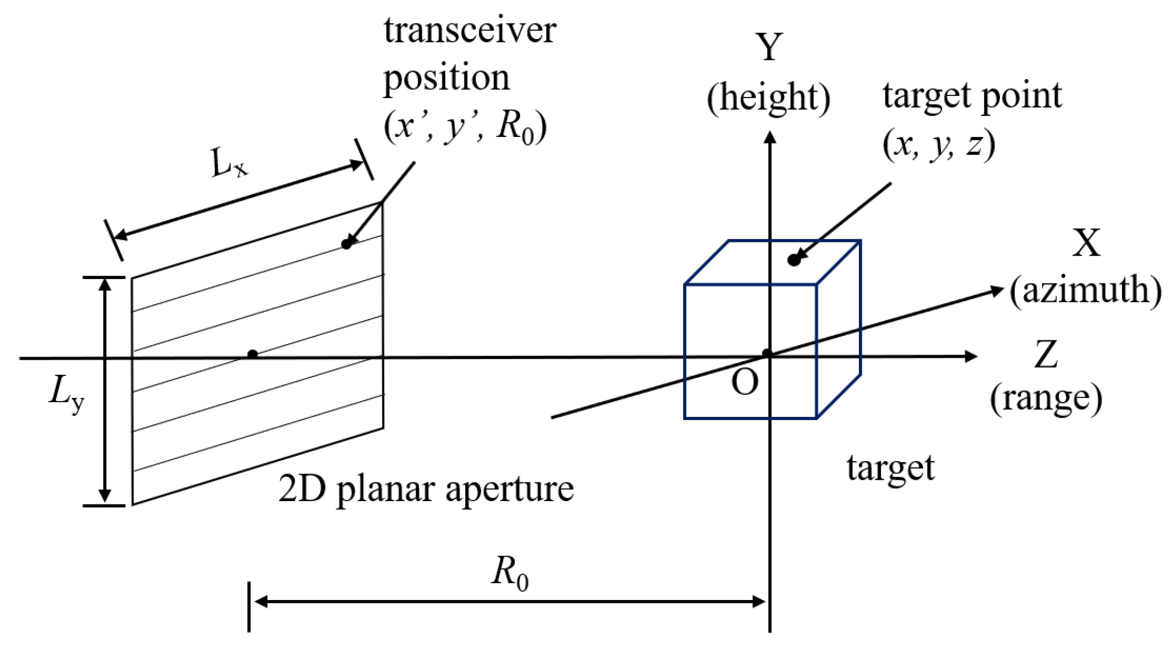
2.1. Three-Dimensional (3D) Range Migration Algorithm

The diagram of the considered MMW close-range imaging system is shown in Figure 1. The motion trajectory of the transceiver is linear. Let $\left(x^{\prime },y^{\prime },R_0\right)$ be a spatial sampling position of the transceiver, where $x^{\prime }\in \left[-L_x/2,L_x/2\right]$ and $y^{\prime }\in \left[-L_y/2,L_y/2\right]$, $L_x$ denotes the aperture length in the azimuth dimension (i.e., X dimension), $L_y$ denotes the aperture length in the height dimension (i.e., Y dimension) and $R_0$ indicates the distance between the observation plane and the target origin.

Assuming that the transceiver emits stepped-frequency (SF) signals, at the p-th frequency, the response measured at the transceiver is

$$s\left(x^{\prime },y^{\prime },k_p\right) = \underset{x,y,z}{\int \int \int }\sigma \left(x,y,z\right)e^{-j2k_{p}R}dxdydz,$$

(1)

where $\sigma \left(x,y,z\right)$ denotes the reflectivity function of the scatterer at the position $(x,y,z)$,$k_p = 2\pi f_p/c$ denotes the wave-number, c denotes the speed of light, $f_p$ denotes the p-th operating frequency, $f_p = f_0 + \left(p - 1\right)\mathrm{\Delta }f$, $f_0$ and $\mathrm{\Delta }f$ denote the starting frequency and the frequency step, respectively, $p = 1,2,\cdots ,P$ and P is the number of the transmitted stepped frequency, R denotes the distance between the target and the transceiver, i.e., $R = \sqrt{{\left(x - x^{\prime }\right)}^2 + {\left(y - y^{\prime }\right)}^2 + {\left(z - R_0\right)}^2}$. The RMA imaging algorithm is shown in Algorithm 1 [15,16,17].

Although $k_x$, $k_y$ and $k_p$ are uniform, the wave-number component in the Z dimension, i.e., $k_z = \sqrt{4k_p^2 - k_x^2 - k_y^2}$, is non-uniform. The wave-number domain for a certain height is shown in Figure 2. Therefore, the 3rd stage in Algorithm 1 is necessary to achieve the conversion from a non-uniformity of $k_z$ to a uniform one. As Algorithm 1 shows, the echo data $s(x^{\prime },y^{\prime },k_p)$ is transformed into the image data $\widehat{\sigma }(x,y,z)$ through a series of stages, i.e., two-dimensional (2D) Fourier transforms (FT), phase compensation, interpolation, and 3D inverse FT. Highly complete program libraries such as faster Fourier transform in the west (FFTW) and CUDA fast Fourier transform (CUFFT) can efficiently perform FFT operations on the CPU and GPU, respectively. Although CUDA provides a ready-made library of FFT to call, a zero-frequency component transfer operation is required before and after the FT in the program. This operation can be considered a 3D data replication. The time overhead of the data replication operation in the memory is greater than that in the video memory. Moreover, the FFTW library has a very short running time on the CPU. In this paper, the FFTW library is used to achieve efficient operations of the involved Fourier transform. Therefore, the acceleration of interpolation is crucial for imaging.

Algorithm 1 3D RMA imaging

Input: Echoes collected over the frequency band and the whole spatial observation plane, $s\left(x^{\prime },y^{\prime },k_p\right)$,$p = 1,2,\cdots ,P$, $x^{\prime }\in \left[-L_x/2,L_x/2\right]$, $y^{\prime }\in \left[-L_y/2,L_y/2\right]$; Output: 1: Take the spatially 2D FT of $s\left(x^{\prime },y^{\prime },k_p\right)$ along $x^{\prime }$ and $y^{\prime }$ to form the angular spectrum at each frequency, $$\begin{array}{c}\hfill S(k_x,k_y,k_p) = \underset{x^{\prime },y^{\prime }}{\int \int }s(x^{\prime },y^{\prime },k_p)e^{-j(k_x{x}^{\prime } + k_y{y}^{\prime })}d{x}^{\prime }d{y}^{\prime }\end{array}$$ (2) where $k_x$ and $k_y$ denote the wave-number component corresponding to the X-dimension and Y-dimension, respectively. 2: Apply the phase compensation to the angular spectrums based on the method of stationary phase, $$S(k_x,k_y,k_z) = S(k_x,k_y,k_p)e^{-j{k}_z{R}_0}$$ (3) where $k_z$ denotes the wave-number component corresponding to the Z-dimension, and, and $k_z = \sqrt{4k_p^2 - k_x^2 - k_y^2}$. 3: Turn the non-uniform $S(k_x,k_y,k_z)$ to the uniform $\dot{S}(k_x,k_y,{\dot{k}}_z)$ by cubic spline interpolation, where $\dot{S}(k_x,k_y,{\dot{k}}_z)$ denotes the spectrum value at the position $(k_x,k_y,{\dot{k}}_z)$ and ${\dot{k}}_z$ denotes the desired uniform sampling position of the wave-number component in the Z-dimension. 4: Take the 3D inverse FT of $\dot{S}(k_x,k_y,{\dot{k}}_z)$ to achieve the imaging, $$\widehat{\sigma }(x,y,z) = \frac{1}{{\left(2\pi \right)}^3}\underset{k_x,k_y,k_z}{\int \int \int }\dot{S}(k_x,k_y,{\dot{k}}_z)e^{j(k_{x}x + k_{y}y + k_{z}z)}d{k}_{x}d{k}_{y}d{k}_z$$ (4) 5: return: $\widehat{\sigma }(x,y,z)$

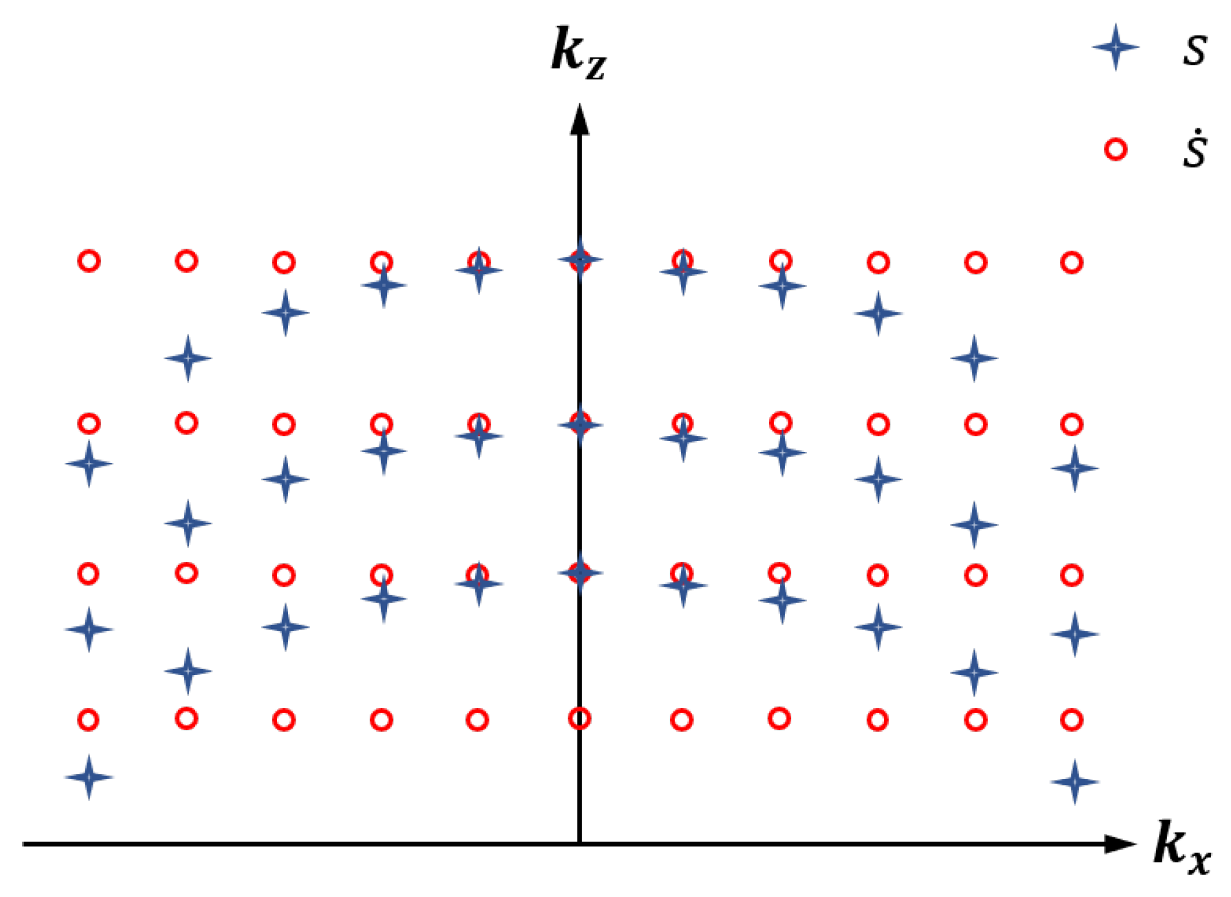
2.2. Cubic Spline Interpolation

To discuss the interpolation, the Algorithm 1 would be discretized. The transceiver is sampled uniformly in the azimuth and height dimensions, and the $(m,n)$-th sampling position is denoted as $(x_m,y_n)$, where $x_m = -L_x/2 + (m - 1)d_x$, $m = 1,2,\cdots ,M$, $x_m\in \left[-L_x/2,L_x/2\right]$; $y_n = -L_y/2 + (n - 1)d_y$, $n = 1,2,\cdots ,N$, $y_n\in \left[-L_y/2,L_y/2\right]$; $d_x$ and $d_y$ denote the sampling intervals in the azimuth and height dimensions, respectively. Then, stacking all the samples of $S\left(k_x,k_y,k_z\right)$ in Equation (3) gives,

$$\begin{array}{c}\hfill \mathit{S} = {\left[\begin{array}{ccc}S(k_{x,1},k_{y,1},k_{z,(1,1,1)})& \cdots & S(k_{x,1},k_{y,1},k_{z,(1,1,P)})\\ ⋮& \ddots & ⋮\\ S(k_{x,M},k_{y,1},k_{z,(M,1,1)})& \cdots & S(k_{x,M},k_{y,1},k_{z,(M,1,P)})\\ ⋮& \ddots & ⋮\\ S(k_{x,M},k_{y,N},k_{z,(M,N,1)})& \cdots & S(k_{x,M},k_{y,N},k_{z,(M,N,P)})\end{array}\right]}_{MN \times P}\end{array}$$

(5)

where $k_{z,(m,n,p)} = \sqrt{4k_p^2 - k_{x,m}^2 - k_{y,n}^2}$. The 1D interpolation of $\mathit{S}$ is done along the $k_z$-dimension. Let ${\mathit{s}}_{m,n}$ be the column vector of the $(m + (n - 1\left)M\right)$-th row, i.e., ${\mathit{s}}_{m,n} = {[S(k_{x,m},k_{y,n},k_{z,(m,n,1)}),\cdots ,S(k_{x,m},k_{y,n},k_{z,(m,n,P)})]}^T$. Since $k_x$, $k_y$ have been uniformly sampled and they are invariant in each row, the variables $k_x$ and $k_y$ can be omitted in ${\mathit{s}}_{m,n}$ for simplification. Therefore, for each row, let $\mathit{s}\in C^{P \times 1}$ be the column vector for generalization, and $\mathit{s} = {[s_1,s_2,\cdots ,s_P]}^T$. The p-th element of $\mathit{s}$ corresponds to the wave-number domain component at $k_{z,p}$, and $k_{z,p}$ is non-uniform. Let $\dot{\mathit{s}}\in C^{Q \times 1}$ denote the vector of points after interpolation, i.e., $\dot{\mathit{s}} = {[{\dot{s}}_1,{\dot{s}}_2,\cdots ,{\dot{s}}_Q]}^T$, and the q-th element of $\dot{\mathit{s}}$ corresponds to the wave-number domain component at the desired ${\dot{k}}_{z,q}$, where ${\dot{k}}_{z,q}$ is uniform, $q = 1,2,\cdots ,Q$. It is worth noting that the original set $\{k_{z,p},p = 1,2,\cdots ,P\}$ is different in different rows. Even though $k_{z,p}$ depends on the determined $k_{x,m}$ and $k_{y,n}$ in the $(m + (n - 1\left)M\right)$-th row, the positions to be interpolated is fixed denoted by the common set as $\{{\dot{k}}_{z,q},q = 1,2,\cdots ,Q\}$. The cubic-spline equation at the q-th point to be interpolated can be constructed in the following form Refs. [18,19],

$${\dot{s}}_q = a_p + b_p({\dot{k}}_{z,q} - k_{z,p}) + c_p{({\dot{k}}_{z,q} - k_{z,p})}^2 + d_p{({\dot{k}}_{z,q} - k_{z,p})}^3$$

(6)

where $k_{z,p} < {\dot{k}}_{z,q} < k_{z,p + 1}$, $a_p$, $b_p$, $c_p$, $d_p$ are the zero-order term coefficient, the primary term coefficient, the secondary term coefficient, and the tertiary term coefficient of $({\dot{k}}_{z,q} - k_{z,p})$, respectively. The cubic spline function is shown in Algorithm 2 [18,19,20].

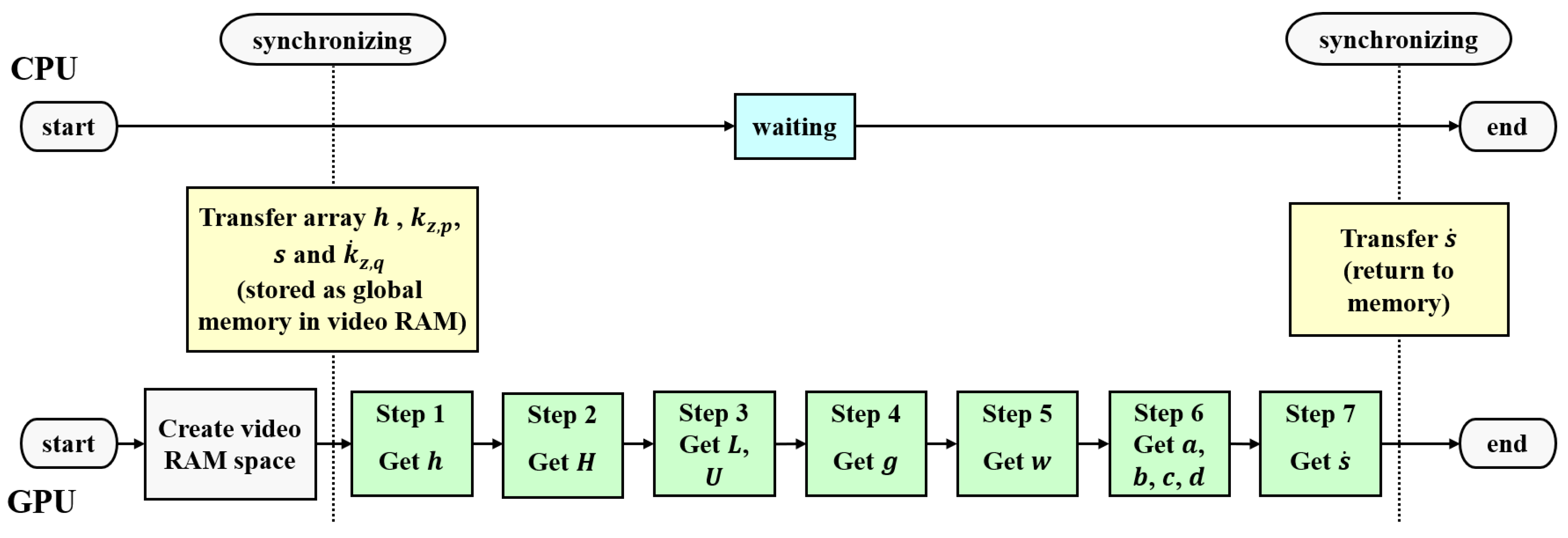
2.3. GPU-Only Method

The scheme for computing the cubic spline interpolation in a GPU-only platform is shown in Figure 3.

In Algorithm 2, although the computations of all the $M \times N$ vectors of $\mathit{s}$ satisfy the program parallelization in the GPU platform, the straightforward migration of the cubic spline interpolation in the GPU would cost a lot of time. This is because that kernel functions in the GPU need to find the adjacent points $k_{z,i}$ of the interpolation point ${\dot{k}}_{z,q}$ and the wave value $s_i$ of $k_{z,i}$. Especially in step 7, kernel functions need to find the address of each ${\dot{s}}_q$ in advance. This traditionally parallel design requires kernel functions of the GPU to run through the entire interpolation process and increases the workload of the video random-access memory (RAM). This method also causes the CPU to stand by for a long time. This is not in line with the solution of the efficient use of the hardware. Although GPUs have a large number of cores, their cores’ structure is too simple to be as fast as CPUs for single instruction single data (SISD) processing.

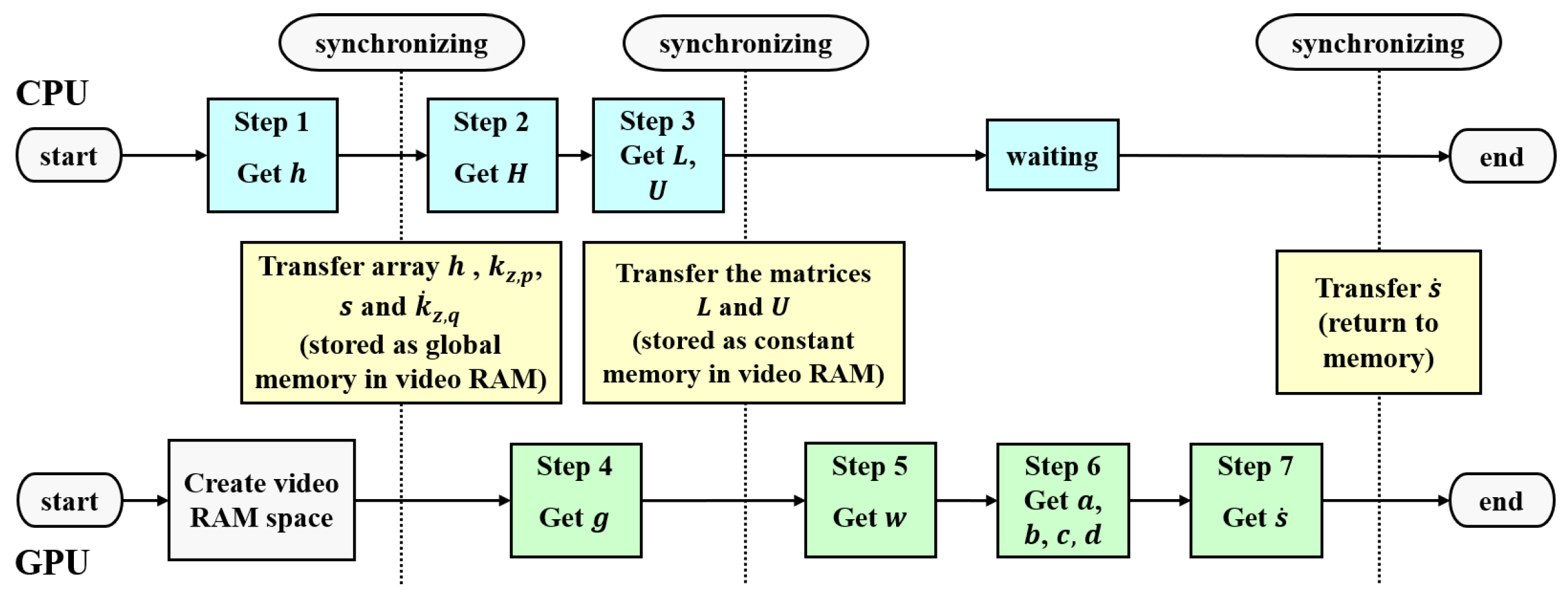
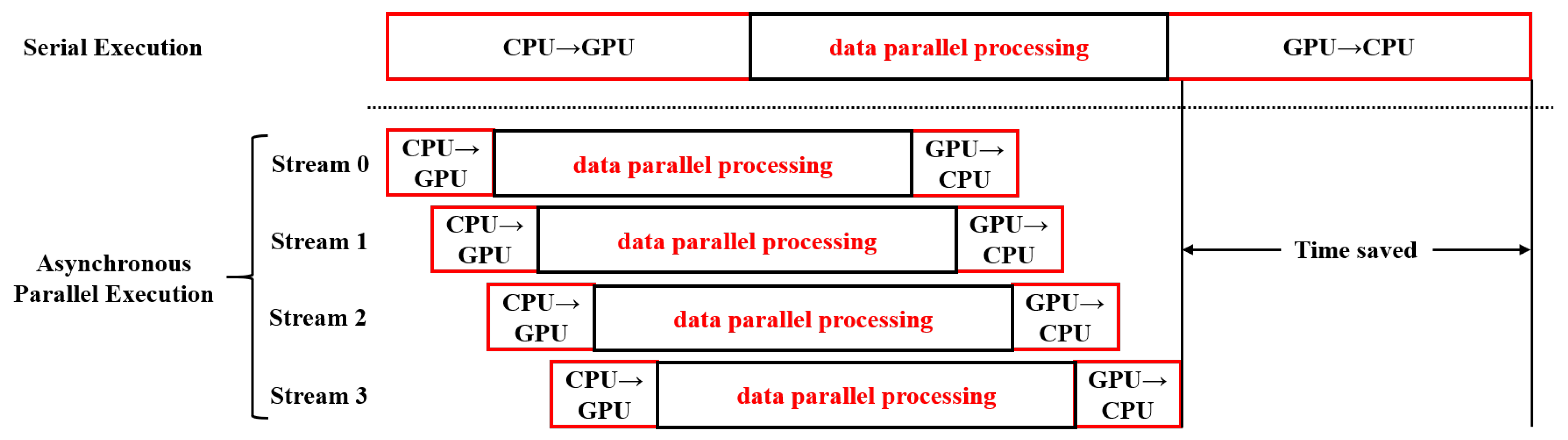
2.4. The Hybrid GPU and CPU Acceleration Method

Since the structural characteristics of the CPU make it better for SISD processing, we use the CPU to perform step 1, step 2, and step 3 of the Algorithm 2 which are suited for the SISD computation model, and put the other steps into the GPU for processing. In step 7, when kernel functions interpolate each row of the echo data $\mathit{S}$ through a parallel processing scheme, the GPU-only method causes additional waiting time for kernel functions to find the ${\dot{s}}_q$. The proposed method utilizes the sequential addressing ${\dot{s}}_q$ of ${\dot{k}}_{z,q}$. This way avoids extra waiting time for different kernel functions to find ${\dot{s}}_q$, thus speeding up the whole program. The optimized schematic block diagram is shown in Figure 4.

Algorithm 2 Cubic spline function

Input: The originally non-uniform sampling positions in $k_z$-dimension, i.e., $k_{z,p},p = 1,2,\cdots ,P$; 1D column vector to be interpolated, $\mathit{s}\in C^{P \times 1}$; The desired uniform positions ${\dot{k}}_{z,q},q = 1,2,\cdots ,Q$; Output: 1: Calculate the z-dimension difference, denotes $h_i,i = 1,2,\cdots ,P - 1$; $$h_i = k_{z,i + 1} - k_{z,i}$$ (7) 2: Construct the tridiagonal matrix $\mathit{H}$ from the obtained $h_i$ $$\mathit{H} = \left[\begin{array}{cccccc}1& 0& 0& \cdots & \cdots & 0\\ h_1& 2(h_1 + h_2)& h_2& \cdots & \cdots & 0\\ \cdots & \cdots & \cdots & \cdots & \cdots & \cdots \\ 0& \cdots & \cdots & h_{P - 2}& 2(h_{P - 2} + h_{P - 1})& h_{P - 1}\\ 0& \cdots & \cdots & 0& 0& 1\end{array}\right]$$ (8) 3: Decompose $\mathit{H}$ using Gaussian elimination to obtain the upper triangular matrix $\mathit{L}$ and the lower triangular matrix $\mathit{U}$. 4: Calculate the matrix $\mathit{g}$ based on the following formula, $$\mathit{g} = 6{\left[\begin{array}{cccccc}0& \frac{s_3 - s_2}{h_2} - \frac{s_2 - s_1}{h_1}& \frac{s_4 - s_3}{h_3} - \frac{s_3 - s_2}{h_2}& \cdots & \frac{s_P - s_{P - 1}}{h_{P - 1}} - \frac{s_{P - 1} - s_{P - 2}}{h_{P - 2}}& 0\end{array}\right]}^T$$ (9) 5: Construct the vector $\mathit{w},\mathit{w} = {[w_1,w_2,\cdots ,w_P]}^T$ based on the following formula, where $w_p$ denotes the quadratic differential value of $s_p$, i.e., $w_p = s_p^{\prime \prime }$. $$\mathit{w} = {\mathit{U}}^{-1}{\mathit{L}}^{-1}\mathit{g}$$ (10) 6: Determine the coefficients in Equation (6) from the obtained $h_i$ and $w_i$ based on the following equation: $$a_i = s_i$$ (11) $$b_i = \frac{s_{i + 1} - s_i}{h_i} - \frac{h_i{w}_i}{2} - \frac{h_i(w_{i + 1} - w_i)}{6}$$ (12) $$c_i = \frac{w_i}{2}$$ (13) $$d_i = \frac{w_{i + 1} - w_i}{6h_i}$$ (14) 7: Estimate the spectrum of ${\dot{s}}_q$ correspond to ${\dot{k}}_{z,q}$, baesd on Equation (6), $${\dot{s}}_q = a_i + b_i({\dot{k}}_{z,q} - k_{z,i}) + c_i{({\dot{k}}_{z,q} - k_{z,i})}^2 + d_i{({\dot{k}}_{z,q} - k_{z,i})}^3$$ (15) where $k_{z,i} < {\dot{k}}_{z,q} < k_{z,i + 1}$. 8: return: $\dot{\mathit{s}} = {[{\dot{s}}_1,{\dot{s}}_2,\cdots ,{\dot{s}}_Q]}^T$

The pseudo code is shown in the Algorithm 3:

Algorithm 3 Hybrid CPU-GPU method pseudo code of cubic spline interpolation

Input: The originally non-uniform sampling positions in $k_z$-dimension, i.e., $k_{z,p},p = 0,2,\cdots ,P - 1$; 1D column vector to be interpolated, $\mathit{s}\in C^{P \times 1}$; The desired uniform positions ${\dot{k}}_{z,q},q = 0,2,\cdots ,Q - 1$; Output: 1: for$p[0:P - 2]$do 2:      $h\left[p\right] = k_{z,p + 1} - k_{z,p}$⟵ Calculation of wave number domain steps, i.e., Equation (7) 3: end for 4: for$p[1:P - 3]$do 5:      $H1\left[p\right] = h[p - 1]$ 6:      $H2\left[p\right] = \left(h\right[p - 1] + h[p\left]\right) \ast 2$ 7:      $H3\left[p\right] = h\left[p\right]$⟵ Calculation of the three diagonals of the tridiagonal matrix $\mathit{H}$, i.e., Equation (8) 8: end for 9: $H1[P - 3] = 0.0,H2\left[0\right] = H2[P - 1] = 1.0,H3\left[0\right] = 0.0$ 10: $U\left[0\right] = H2\left[0\right]$ 11: for$p[1:P - 4]$do 12:      $L\left[p\right] = H1\left[p\right]/U[p - 1]$ 13:      $U\left[p\right] = H2\left[p\right] - H3[p - 1] \ast L\left[p\right]$ 14: end for 15: $L\left[0\right] = H1[P - 4]/U[P - 5]$ 16: Use the function cudaMemcpyToSymbol to send $\mathit{L},\mathit{U},\mathit{h}$ to constant memory.         17: $id⟵blockDim.x \ast blockIdx.x + threadIdx.x$    (GPU running part) 18: $g\left[id\right] = 6 \ast (\frac{s[id + 1] - s\left[id\right]]}{h\left[id\right]} - \frac{s\left[id\right] - s[id - 1]}{h[id - 1]})$⟵ Computing the array g, i.e., Equation (9) 19: $Uw\left[id\right] = g\left[id\right] - L\left[id\right]*Uw[id - 1]$ ⟵ Computing the array $\mathit{Uw}$. The array $\mathit{Uw}$ is an intermediate step in the computation of the array $\mathit{w}$. 20: $w[P - 4] = Uw[P - 4]/U[P - 4]$ 21: $w\left[id\right] = \left(Uw\right[id] - H3[id] \ast w[id + 1\left]\right)/U\left[id\right]$⟵ Computing the array $\mathit{w}$, i.e., Equation (10). 22: $w\left[id\right] = w[id - 1],w\left[0\right] = 0.0,w[P - 2] = 0.0$⟵ Add 0 to both ends of array $\mathit{w}$. 23: $a\left[id\right] = s\left[id\right]$ 24: $b\left[id\right] = \frac{s[id + 1] - s\left[id\right]}{h\left[id\right]} - \frac{h\left[id\right] \ast w\left[id\right]}{2} - \frac{h\left[id\right] \ast \left(w\right[id + 1] - w[id\left]\right)}{6}$ 25: $c\left[id\right] = w\left[id\right]/2$ 26: $d\left[id\right] = \frac{w[id + 1] - w\left[id\right]}{6 \ast h\left[id\right]}$⟵ Calculation of spline curve coefficients, i.e., Equation (11) to Equation (14) 27: if$k_{z,p}$ < ${\dot{k}}_z,q$ < $k_{z,p + 1}$ 28:      ${\dot{s}}_q = a\left[id\right] + b\left[id\right] \ast ({\dot{k}}_{z,q} - k_{z,i}) + c\left[id\right] \ast {({\dot{k}}_{z,q} - k_{z,i})}^2 + d\left[id\right] \ast {({\dot{k}}_{z,q} - k_{z,i})}^3$⟵ Calculation of the spatial wave number at the interpolation point, i.e., Equation (15) 29: end if 30: return: $\dot{\mathit{s}} = {[{\dot{s}}_0,{\dot{s}}_1,\cdots ,{\dot{s}}_{Q - 1}]}^T$

The pseudo-code corresponds to Algorithm 2. The step 1 to step 3 of the Algorithm 2 are calculated in the CPU. The CPU transfers the matrices $\mathit{L}$ and $\mathit{U}$ to the video memory after completing step 3. Generally, this task can be approached with different mechanisms: global memory, shared memory, texture memory, and constant memory. To avoid the time-consuming impact of access conflicts on the overall cubic spline interpolation, the matrices $\mathit{L}$ and $\mathit{U}$ are stored in constant memory.

Generally speaking, the memory is much larger than the video memory. In the implementation of CUDA kernel functions, the data is transferred from the memory to the video memory, which requires data transfer time. The data are then read from the video memory and processed using multiple threads, which requires computation time. Therefore, the time consumed to execute the algorithm is the sum of the data transfer time and the computation time. Before running the signal processing, it is necessary to reduce the data transfer time. For large amounts of data, it is not possible to transfer the data in the CPU buffer to the GPU at one time. Therefore, it needs to be transferred in chunks. If it is desired to perform kernel function operations on the GPU at the same time as data transfer, streams can be introduced for asynchronous parallel processing of data to improve computational performance.

Therefore, in our close-range 3D imaging, the proposed method in this paper utilizes asynchronous parallelism for data processing, which is different from the common serial execution method. Actually, the implementation of the asynchronous parallel scheme is shown in Figure 5, which compares the running time of both the serial execution and the 4-stream asynchronous parallel execution. As Figure 5 shows, 4 streams are created in the GPU, and the data transferred from the CPU is equally distributed to each stream. In such a way, the data transfer and processing among different streams would not interfere with each other. This allows the data interaction between memory and video memory to be executed in parallel with the computation of kernel functions. This approach ensures that the GPU core is busy most of the time while effectively alleviating the drawback of a long time for data transfer between the memory and video memory.

Because of the semi-threaded bundle broadcast feature of the constant memory, the GPU reads constant memory much faster than global memory. Therefore, the choice of constant memory saves a theoretical $93.75\%$ of read time. The left steps 4–7 would be achieved in the GPU. These 1D data in each row meet the parallelism requirement and can be processed in parallel by the GPU’s single instruction multiple data (SIMD) processing capability.

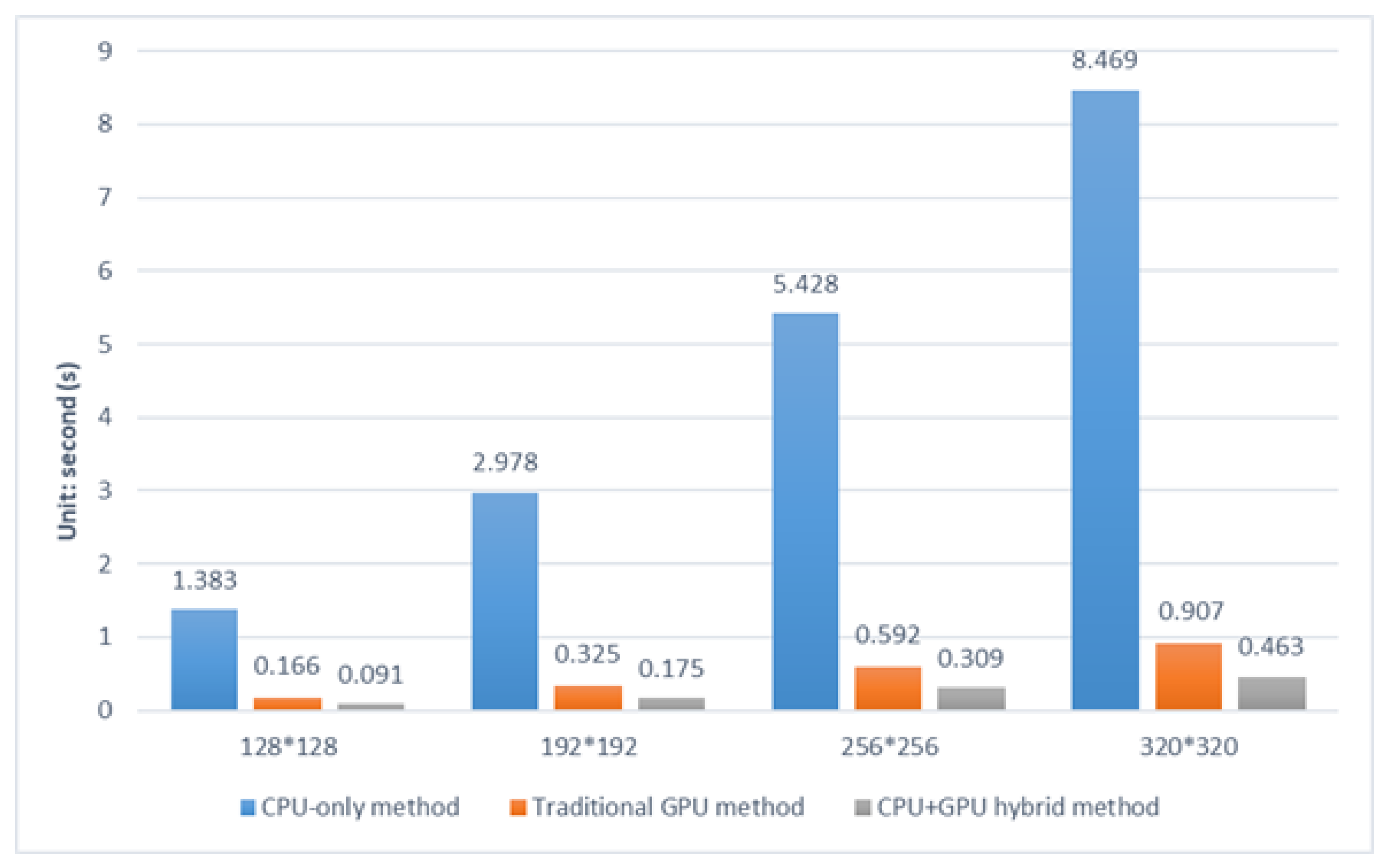
3. Experimental Results and Analysis

Simulation experimental configuration: Inter(R) Core(TM) i5-7400 CPU @ 3.00GHz processor; 64-bit operating system; 16G memory (RAM); 1 NVIDIA GTX 1050 4G GDDR5 discrete graphics card; 1 PNA network analyzer. The measurement parameters used in the experiment are listed in

Table 1. Measurement parameters used in the simulation and the experiment.

Parameters	Value
Center frequency	92.5 GHz
Frequency bandwidth	35 GHz
Sweeping frequency points	201
azimuth dimension samples number	161
azimuth dimension sampling interval	1.5 mm
azimuth dimension aperture length	0.24 m
height dimension samples number	161
height dimension sampling interval	1.5 mm
height dimension aperture length	0.24 m
Antenna beamwidth	30∘
Antenna-to-target distance	0.3 m

. The single point simulation experimental scenarios and results are shown in Figure 6.

To verify the correctness of the results, the 3D RMA close-range imaging algorithm is implemented by CPU-only, GPU-only and our proposed method, respectively. In this paper, MATLAB, a commercial mathematical software from MathWorks, is used as the imaging display platform. According to Figure 6, results obtained from the simulation, the difference among these 3 methods is quite small. Next, the actual imaging experiments are performed, which the same parameters as the simulation model parameters. The experimental scenarios and results are shown in Figure 7 and Figure 8. It is clearly observed from the comparison in Figure 8 that the imaging algorithm can be implemented properly on different platforms. Thus, it confirms the feasibility of our proposed approach.

The amplitude-level comparison between the two methods is shown in Figure 9. In Figure 9, the 3D surface is created using MATLAB’s built-in mesh function so that the energy distribution of the main view in Figure 8 can be visualized. From this, the imaging results calculated by these two methods can be found without significant differences. The absolute error is only about $1.11628 \times {10}^{-6}$, which confirms that the proposed method can meet the functional requirements.

Figure 10 depicts the time consumption by different platforms with various data sizes.

Table 2. Speedup ratio of the traditional GPU-only method and the hybrid CPU + GPU method compared to the CPU-only method.

Data Volume	128 × 128	192 × 192	256 × 256	320 × 320
Methods
Traditional GPU method	8.33	9.16	9.17	9.34
CPU+GPU hybrid method	15.20	17.02	17.57	18.30

summarizes the speedup ratios of the conventional GPU-only method and the hybrid CPU+GPU method compared to the CPU-only method.

Since the GPU programs have a start-up overhead, the benefits of the GPU-based parallel acceleration can only be realized when the amount of data is large enough. From Table 2, we can have that the program with the traditional GPU parallel acceleration method gets more than 8 times the speedup ratio compared to the CPU-only method. The hybrid CPU + GPU method makes the speedup ratio reach more than 15 times, and the results demonstrate that the larger the data size is, the better acceleration the method can reach.

4. Conclusions

In this paper, we conduct an in-depth study of hardware optimization for the 3D RAM implementation on the CUDA platform with the programmable GPU and elaborate a hybrid GPU and CPU strategy to achieve parallel computing. Especially for the interpolation stage which has the greatest influence on the imaging time efficiency, this paper uses four streams to optimize the data transfer and selects different video memory for storage according to the data characteristics, optimizes the matrix storage method, and accomplishes the effective execution of RMA. The calculation results using the NVIDIA GTX 1050 graphics card demonstrate that the calculation speed of the MMW 3D close-range imaging based on our acceleration optimization is greatly improved compared to the CPU-only platform and the traditional GPU-only method. Lastly, we accompany our contribution with the full source code of a working prototype (the code and explanatory notes can be accessed via the following URL: https://github.com/miao3rd/miao_c.git accessed on 24 January 2023).

References

1. Lorente, D.; Limbach, M.; Gabler, B.; Esteban, H.; Boria, V.E. Sequential 90° rotation of dual-polarized antenna elements in linear phased arrays with improved cross-polarization level for airborne synthetic aperture radar applications. Remote Sens. 2021, 13, 1430. [Google Scholar] [CrossRef]
2. Liu, C.; Chen, Z.; Yun, S.; Chen, J.; Hasi, T.; Pan, H. Research advances of SAR remote sensing for agriculture applications: A review. J. Integr. Agric. 2019, 18, 506–525. [Google Scholar] [CrossRef]
3. Alibakhshikenari, M.; Virdee, B.S.; Limiti, E. Wideband planar array antenna based on SCRLH-TL for airborne synthetic aperture radar application. J. Electromagn. Waves Appl. 2018, 32, 1586–1599. [Google Scholar] [CrossRef]
4. Li, J.; Song, L.; Liu, C. The cubic trigonometric automatic interpolation spline. IEEE/CAA J. Autom. Sin. 2017, 5, 1136–1141. [Google Scholar] [CrossRef]
5. Liu, J.; Qiu, X.; Huang, L.; Ding, C. Curved-path SAR geolocation error analysis based on BP algorithm. IEEE Access 2019, 7, 20337–20345. [Google Scholar] [CrossRef]
6. Miao, X.; Shan, Y. SAR target recognition via sparse representation of multi-view SAR images with correlation analysis. J. Electromagn. Waves Appl. 2019, 33, 897–910. [Google Scholar] [CrossRef]
7. Kim, B.; Yoon, K.S.; Kim, H.-J. GPU-Accelerated Laplace Equation Model Development Based on CUDA Fortran. Water 2021, 13, 3435. [Google Scholar] [CrossRef]
8. Yin, Q.; Wu, Y.; Zhang, F.; Zhou, Y. GPU-based soil parameter parallel inversion for PolSAR data. Remote Sens. 2020, 12, 415. [Google Scholar] [CrossRef]
9. Cui, Z.; Quan, H.; Cao, Z.; Xu, S.; Ding, C.; Wu, J. SAR target CFAR detection via GPU parallel operation. IEEE J. Sel. Top. Appl. Earth Obs. Remote Sens. 2018, 11, 4884–4894. [Google Scholar] [CrossRef]
10. Liu, G.; Yang, W.; Li, P.; Qin, G.; Cai, J.; Wang, Y.; Wang, S.; Yue, N.; Huang, D. MIMO Radar Parallel Simulation System Based on CPU/GPU Architecture. Sensors 2022, 22, 396. [Google Scholar] [CrossRef] [PubMed]
11. Gou, L.; Li, Y.; Zhu, D. A real-time algorithm for circular video SAR imaging based on GPU. Radar Sci. Technol. 2019, 17, 550–556. [Google Scholar]
12. Liu, J.; Yang, B.; Su, Y.; Liu, P. Fast Context-Adaptive Bit-Depth Enhancement via Linear Interpolation. IEEE Access 2019, 7, 59403–59412. [Google Scholar] [CrossRef]
13. Carnicer, J.M.; Khiar, Y.; Peña, J.M. Inverse central ordering for the Newton interpolation formula. Numer. Algorithms 2022, 90, 1691–1713. [Google Scholar] [CrossRef]
14. Chand, A.; Kapoor, G. Cubic spline coalescence fractal interpolation through moments. Fractals 2007, 15, 41–53. [Google Scholar] [CrossRef]
15. Wang, Z.; Guo, Q.; Tian, X.; Chang, T.; Cui, H.-L. Near-Field 3-D Millimeter-Wave Imaging Using MIMO RMA with Range Compensation. IEEE Trans. Microw. Theory Tech. 2019, 67, 1157–1166. [Google Scholar] [CrossRef]
16. Sheen, D.; McMakin, D.; Hall, T. Near-field three-dimensional radar imaging techniques and applications. Appl. Opt. 2010, 49, E83–E93. [Google Scholar] [CrossRef] [PubMed]
17. Tan, W.; Huang, P.; Huang, Z.; Qi, Y.; Wang, W. Three-dimensional microwave imaging for concealed weapon detection using range stacking technique. Int. J. Antennas Propag. 2017, 2017, 1480623. [Google Scholar] [CrossRef]
18. Kapoor, G.P.; Prasad, S.A. Convergence of Cubic Spline Super Fractal Interpolation Functions. Fractals 2012, 22, 218–226. [Google Scholar]
19. Abdulmohsin, H.A.; Wahab, H.B.A.; Hossen, A.M.J.A. A Novel Classification Method with Cubic Spline Interpolation. Intell. Autom. Soft Comput. 2022, 31, 339–355. [Google Scholar] [CrossRef]
20. Viswanathan, P.; Chand, A.; Agarwal, R.P. Preserving convexity through rational cubic spline fractal interpolation function. J. Comput. Appl. Math. 2014, 263, 262–276. [Google Scholar] [CrossRef]
Figure 1. Close-range imaging.
Electronics 12 00840 g001
Figure 2. The wave-number domain of a certain height.
Electronics 12 00840 g002
Figure 3. Cubic spline interpolation in the traditionally GPU-only platform.
Electronics 12 00840 g003
Figure 4. The proposed method.
Electronics 12 00840 g004
Figure 5. Asynchronous parallel execution and serial execution.
Electronics 12 00840 g005
Figure 6. Azimuth amplitude results. (a) is the CPU implementation result; (b) is the GPU implementation result; (c) is the result of the proposed method implementation.
Electronics 12 00840 g006
Figure 7. Experimental scene.
Electronics 12 00840 g007
Figure 8. Imaging results comparison. (ac) are the front, top and side views obtained by CPU-only method, respectively; (df) are the front, top and side views obtained by GPU-only method, respectively; (gi) are the front, top and side views obtained by the proposed method, respectively.
Electronics 12 00840 g008
Figure 9. Amplitude-level comparison. (a) is the imaging target energy map obtained by the CPU-only method; (b) is the imaging target energy map obtained by the GPU-only method; and (c) is the imaging target energy map obtained by the proposed method.
Electronics 12 00840 g009
Figure 10. Comparison of the time consumption by different platforms.
Electronics 12 00840 g010