Improved A-Star Path Planning Algorithm in Obstacle Avoidance for the Fixed-Wing Aircraft

Abstract

The flight management system is a basic component of avionics for modern airliners. However, the airborne flight management system needs to be improved and relies on imports; path planning is the key to the flight management system. Based on the classical A* algorithm, this paper proposes an improved A* path planning algorithm, which solves the problem of low planning efficiency and following a non-smooth path. In order to solve the problem of the large amount of data calculation and long planning time of the classical A* algorithm, a new data structure called a “value table” is designed to replace the open table and close table of the classical A* algorithm to improve the retrieval efficiency, and the Heap sort algorithm is used to optimize the efficiency of node sorting. Aiming at the problem that the flight trajectory is hard to follow, the trajectory smoothing optimization algorithm combined with turning angle limit is proposed. The gray value in the digital map is added to the A* algorithm, and the calculation methods of gray cost, cumulative cost, and estimated cost are improved, which can better meet the constraints of obstacle avoidance. Through the comparative simulation verification of the algorithm, the improved A* algorithm can significantly reduce the path planning time to 1% compared to the classical A* algorithm; it can be seen that the proposed algorithm improves the efficiency of path planning and the smoother planned path, which has obvious advantages compared to the classical A* algorithm.

1. Introduction

The onboard flight management system (FMS) is a professional computer system that can automate various flight tasks and reduce manual workload. Modern civil aircraft crews no longer carry flight engineers or navigators. However, the FMS for general civil aviation aircraft is dependent on the introduction from abroad [1]. FMS is a basic component of airborne avionics, which can realize the automation of various flight tasks. Its main function is to position the aircraft, make flight plans, optimize routes, guide aircraft flight, and reduce the working pressure of crew.

The civil aviation aircraft is prone to environmental collisions and crashes in the case of low visibility in the air, and emergency landing in mountainous terrain. The China International Airlines Flight 129 crash was due to low visibility in the air; its scheduled route error caused the passenger plane to crash into the mountain, and 129 people were unfortunately killed. Different from the traffic warning and obstacle avoidance system (TACS), airborne obstacle avoidance system (ACSA), and near-Earth warning system (GPWS) [2], FMS performs path planning when facing obstacles that may appear in advance, reducing the accident rate of civil aircraft in complex environments such as mountain flight and multi-aircraft flight. An important performance index of FMS is its planning and obstacle avoidance ability when flying in complex terrain environments.

Path planning is one of the core functions of FMS. The autonomous auxiliary path planning for civil aircraft in emergency flight will significantly help the aircraft to guide the emergency landing in bad weather, complex terrain, and sudden accidents, and decrease the incidence of major air crashes.

The path planning algorithm includes two parts: a map preprocessing algorithm and pathfinding algorithm [3]. Digital map processing needs to select the corresponding processing method according to the different elevation data and task requirements. For maps with different accuracy, it is necessary to process the best digital map suitable for the pathfinding algorithm. At present, there are many pathfinding algorithms for path planning. The A* algorithm is one of the most representative heuristic algorithms [4]. Its success rate and superiority of algorithm results are incomparable to other algorithms. However, there are still many directions for optimization of the algorithm. The computational complexity of the algorithm is related to the accuracy of the map. The higher the accuracy of the map, the greater the amount of calculation of the planning algorithm caused by the surge in data volume. The large amount of calculation also causes excessive space memory occupation, and the large amount of data will lead to problems such as program collapse in engineering. The classical A* algorithm cannot add the aircraft performance limit to the track, the planned track helicopter is difficult to follow, and the degree of engineering is low; at present, the application of the A* algorithm only stays in the calculation of an unselectable single track, and cannot be reasonably adjusted according to the task situation.

Many scholars have conducted a lot of research on how to improve the efficiency of the map preprocessing algorithm and pathfinding algorithm. The key step of path planning for robots, including UAVs, is to accurately process map information [5] and reach the target without collision [6]. Jaishankar et al. [7] proposed a distance change method, through which the digital elevation can be represented by grayscale image, and the path planning can be carried out on this basis. Meng H [8] first smoothed and optimized the data in the digital map from four directions, then processed the digital map into the smallest threat surface, and then sought the optimal path on the smallest threat surface. The algorithms lack the interpolation calculation of the appropriate accuracy of the map first, which may result in the situation that the resolution of the elevation data is not enough to support the pathfinding algorithm, or the resolution is too high to cause the data to be too large and the efficiency of the algorithm to be reduced.

The path planning algorithm not only requires that the planned flight path is feasible, but also requires its optimality in some specific criteria, such as calculation time and trajectory length [9]. The calculation time mainly includes map processing time and path planning time, which will be mainly used as the evaluation criteria for different algorithms in this paper. The A* algorithm is a famous algorithm in the field of path planning, which is suitable for the static environment exploration of complex obstacle topographic map [10]. However, the classical A* algorithm is not satisfactory in terms of computational time [11], which seriously hinders the deployment of the A* algorithm and its application in the actual aircraft navigation system. On this basis, many studies have proposed methods to improve the computational performance. Sudhakara et al. [12] proposed an improved A* algorithm to increase the number of turns to plan the path of the robot in a position environment with obstacles. Pal et al. [13] proposed an improved A* algorithm based on capacity consumption to reduce the energy consumption caused by stopping and turning.

In addition to considering the calculation length and trajectory time, the performance requirements of fixed-wing aircraft should be met when planning the path. ElHalawany et al. [14] proposed an improved A* algorithm considering its own size to avoid sharp turns in the path planning of mobile robots, which is necessary in practical applications. Based on the traditional algorithm, this paper adds the constraints of fixed-wing aircraft performance, so that the planned trajectory is easy to follow. In order to improve the performance of fixed-wing aircraft, Durán-Delfín et al. [15] established a mathematical model of fixed-wing convertible vertical take-off and landing aircraft to achieve two flight states along the trajectory. The controller has good performance and can provide sufficient maneuverability. This research will greatly improve the performance of fixed-wing aircraft in the future.

At present, the application of the A* algorithm only stays on the calculation of an unselected single trajectory, considering the minimization of multi-objectives such as path length and altitude [16]. However, for fixed-wing aircraft, the requirements for different costs are different under different flight conditions. Ducho et al. [11] modified the A* algorithm and optimized the algorithm based on the complexity of the environment, so that the algorithm can be applied to various scenarios. Aiming at this problem, this paper optimizes the weights of different costs in the cost function.

The main innovations and contributions of this paper are as follows: (1) Aiming at the problems of large memory occupation and high map accuracy requirements in the path planning of fixed-wing passenger aircraft, the digital map is combined with the requirement of the step size of the demand point to adjust the map accuracy, and the elevation digital map is processed into a grayscale map in combination with the aircraft climbing angle limit, so as to reduce the memory occupation of the map, thereby reducing the amount of calculation and improving the efficiency of path planning; (2) Aiming at the problem that the planned global trajectory is hard to follow by fixed-wing aircraft, this paper considers the flight constraints of fixed-wing aircraft flying, and processes the track into a followable trajectory that satisfies the turning angle of the aircraft through trajectory smoothing optimization; (3) Aiming at the problem of single trajectory in the traditional A* global path planning algorithm, this paper normalizes the cost parameters in the A* algorithm and opens the setting port. At the same time, different cost weight parameters are set for planning. The mode and the proportion of each cost parameter can be dynamically adjusted according to the task situation to find the optimal path that meets the task requirements and aircraft performance constraints; (4) Aiming at the problem of low efficiency of the classical A* algorithm in array structure sorting, the Heap sorting method is adopted to improve the sorting efficiency, and a new data structure called a “value table” is designed to optimize the search efficiency compared to the open table and close table of the classical A* algorithm, which reduces the complexity of the sorting algorithm and satisfies the real-time requirements of the planning algorithm.

2. Path Planning Problem and Modeling

2.1. Path Planning Problem for Fixed-Wing Aircraft

The path planning problem of fixed-wing aircraft refers to the specific path planning requirements $M(m,h,p)$, from the initial point $B_{g,t}$ to the target point $E_{g,t}$; the sets of optimal motion trajectory points$x_{g,t}$, $T_{B,E}$ can be calculated by the pathfinding algorithm $\varphi \left(B_{g,t} ,E_{g,t}\right)$, which can be described as follows:

$$T_{B,E}=\left\{x_{g,t}\in M\left(m,h,p\right)\left|x_{g,t}=\varphi \left(B_{g,t},E_{g,t}\right)\right.\right\}$$

(1)

Among them, the mission target requirements $M_m$, fixed-wing aircraft performance requirements $M_h$, algorithm performance requirements $M_p$.

In the case of complex mountainous areas, the primary task of global trajectory planning is to ensure the safe flight of the aircraft, and the aircraft can successfully avoid all obstacles; secondly, the planned trajectory of the aircraft should ensure that the maximum pitch angle constraint, the maximum turning angle constraint, and aircraft’s followability are satisfied. At the same time, the planning algorithm should also ensure a certain timeliness.

2.2. Path Planning Optimization Model

2.2.1. Optimized Objective Goal

The path planning problem can be regarded as a kind of constrained optimization problem. Figure 1 is a top view of the track, where we use hollow dots to represent the track points, with the symbol $p_i$. $l_i$ is the cost of flight distance between each track point. The large black dots represent obstacles in the map. For the altitude cost in the track, its expression is similar to flight distance cost.

Objective function commonly used in path planning [17,18] can be described as (2).

$$\underset{\chi }{\min }J={{\displaystyle \int }}_{t_0}^{t_f}({\omega }_1{c}_t^2+{\omega }_2{h}^2+{\omega }_3{f}_T)dt$$

(2)

where $c_t$, $h$, and $f_T$ represent the cost of track length, flight altitude, and threat, respectively. ${\omega }_1$, ${\omega }_2$, ${\omega }_3$ are the cost factors, $\chi$ indicates the flight trajectory from $t_0$ to $t_f$. The optimization goal of path planning studied in this article is to design an optimal path under obstacle avoidance conditions, so as to minimize the cumulative distance cost and altitude cost of the entire flight process. Without involving threat costs, Equation (2) is modified to obtain Formula (3) [19]:

$$\underset{\chi }{\min }{\displaystyle \sum }_{i=1}^n({\omega }_1{l}_i^2+{\omega }_2{h}_i^2)$$

(3)

In the formula, the flight distance $l_i$ from the track point $p_i$ to the point $p_{i+1}$ is expressed, which can be viewed in Figure 1. By reducing the flight distance, the fuel cost of the aircraft can be shortened; $h_i$ indicates the altitude cost between track points $p_i$ and $p_{i+1}$. ${\omega }_1$, ${\omega }_2$represents the weight of each cost, which is generally valued according to task requirements.

2.2.2. Maximum Pitch Angle Constraint

In order to ensure the fastest flight to the target point, the trajectory must be able to meet the constraints of the maximum pitch angle in the longitudinal maneuver of the aircraft, which requires that there can be no trajectory beyond the maximum pitch angle limit between the two trajectory points in the planned trajectory, as shown in Figure 2.

Among them, ${\alpha }_{max}$ presents the maximum pitch angle, and ${\alpha }_{AB}$ represents the pitch angle from track point A to track point B. It can be obtained by the relative height difference $\mathsf{\Delta }{h}_{AB}$, relative horizontal distance $\mathsf{\Delta }{l}_{AB}$ from track point A to track point B.

$${\alpha }_{AB}=\arctan \left(\frac{\Delta h_{AB}}{\Delta l_{AB}}\right), \left|{\alpha }_{AB}\right|\le {\alpha }_{\max }$$

(4)

2.2.3. Maximum Bend Angle Constraint

Aiming at the problem of aircraft flight safety when flying in mountainous terrain, the maximum bend angle of lateral maneuver needs to be constrained. In order to change the course when the aircraft maintains a certain forward flight speed, according to the requirements of turning speed and turning radius, it is necessary to ensure that the turning angle of the track meets the constraint of the maximum turning angle when the distance between the track points is certain, as shown in Figure 3.

In Figure 3, the heading at track point A is represented by ${\phi }_{AB}$, the heading at track point B is represented by ${\phi }_{BC}$, and the heading angle that needs to be changed from track point A to track point B is represented by ${\beta }_{turn}$; that is the turning angle at track point B.

$${\beta }_{turn}={\phi }_{AB}-{\phi }_{BC}, \left|{\beta }_{turn}\right|\le {\beta }_{\max }$$

(5)

2.2.4. Minimum Terrain Clearance Constraint

The distance between the aircraft and the ground should always be greater than the minimum flight height from the ground, so as not to affect the flight safety due to ground buildings, trees, and so on. Therefore, the height difference $\mathsf{\Delta }{h}_A$ between the planned track point height and the ground should meet the requirement as follows:

$$\Delta h_A\ge \Delta h_{\min }$$

(6)

3. Preprocessing of Map Information

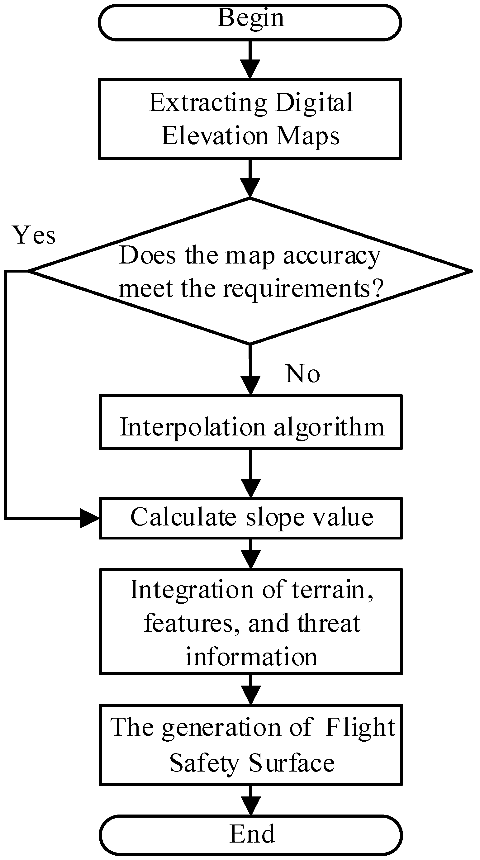
Global path planning is the planning of the aircraft based on the starting point and terrain information before take-off, which requires the terrain data information between the take-off and the end point before take-off, and this information needs to be preprocessed in the three-dimensional space model. The preprocessing algorithm process is shown in Figure 4.

The digital elevation is extracted from the original digital map, and the accuracy information contained in the digital elevation is calculated by using the boundary information and the number of grids. The accuracy requirements of the required digital map are determined by the airborne information storage space and the time requirements for the trajectory planning calculation. The higher the accuracy of the digital map, the greater the storage space required, the longer the calculation time of the track planning, the denser the calculated track points, and the higher the accuracy. The original digital elevation is processed according to the selected map accuracy. If the original digital elevation resolution is too high or too low, it needs to be interpolated to change the resolution of the digital elevation map [18].

In this paper, by reading the high-resolution three-dimensional Digital Elevation Map, the accuracy of the map is adjusted by changing the resolution of the Digital Elevation Model (DEM) through a relatively smooth interpolation algorithm, and the slope value is calculated by the difference algorithm. Combined with the process of slope smoothing and graying, the flight safe surface satisfying the performance constraints such as the climbing rate and the shortest track length of the fixed-wing aircraft could be generated.

3.1. Generation of DEM

The commonly used digital terrain model (DEM) is a mathematical model that describes the parameters such as ground fluctuation and terrain height, and projects the height data of different positions to the data set of the corresponding position on the map in the form of regular gridding or other forms. The model formula is expressed as follows.

$$V_i=\left(g_i,t_i,h_i\right),i=1,2,\cdots ,n$$

(7)

In the above formula, $g_i$ represents the longitude corresponding to the point, $t_i$ represents the latitude corresponding to the point, and $h_i$ represents the height corresponding to the point. In order to construct a three-dimensional space with mountainous terrain, a mountain section was added to the DEM. Merge the original elevation model with mountain data to construct the final spatial 3D model, as shown in the following equation.

$$\begin{array}{l}{V}_i=\left\{g_i,t_i,\max \left[h_i,h_{mt}(g_i,t_i)\right]\right\},i=1,2,\cdots ,n\\ h_{mt}(g_i,t_i)=z_0+{\displaystyle \sum _{j=1}^n{h}_j}\exp \left[\begin{array}{l}-\frac{1}{a^2}{\left(⌊\left(t_i-t_s\right)C_t+\frac{1}{2}⌋-⌊\left(t_0-t_s\right)C_t+\frac{1}{2}⌋\right)}^2\\ -\frac{1}{b^2}{\left(⌊\left(g_i-g_s\right)C_g+\frac{1}{2}⌋-⌊\left(g_0-g_s\right)C_g+\frac{1}{2}⌋\right)}^2\end{array}\right]\end{array}$$

(8)

Among them, the longitude, latitude, and height values $g_i,t_i,h_i$, respectively, of every point in the topographic map are represented; the height of the highest point of the mountain is represented by $z_0$, the slope setting value of the mountain in the $x$ axial direction is represented by $a$, and the slope setting value of the mountain in the $y$ axial direction is represented by $b$. $g_0$, $t_0$ is the longitude and latitude of the highest point of the mountain, respectively; $g_s$, $t_s$ indicates the minimum longitude of the map and the minimum latitude of the map, respectively; $C_g$, $C_t$ represents the amount of data in the longitude direction and the amount of data in the latitude direction, respectively.

3.2. Adjust Map Resolution

Due to the resolution difference caused by the data source of the elevation digital model, the resolution of the elevation data may be insufficient to support the pathfinding algorithm, or the high resolution may lead to excessive data volume and low algorithm efficiency. Therefore, it is necessary to perform linear interpolation on the elevation digital model containing the mountain model to improve or reduce the map accuracy and meet the requirements of different modal pathfinding task algorithms [20,21,22]. The commonly used DEM linear interpolation algorithms are the bilinear interpolation algorithm, bicubic Hermite interpolation algorithm, and two-dimensional cubic convolution interpolation algorithm [23,24].

The interpolation is performed by the above three algorithms, and the graphical comparison results by using the original elevation data are shown in Figure A1, Figure A2, and

Table A1. Data comparison analysis table of interpolation algorithm.

Interpolation Algorithm	Mean (Difference)	Variance (Difference)	Covariance	Correlation Coefficient
Bilinear	−3.3265	496.3242	6729.2543	0.9646
Bicubic Hermite	−3.0499	519.5576	6700.7678	0.9628
2D cubic convolution	−3.0025	434.3359	6746.2220	0.9693

in Appendix B. It can be seen that the mean and variance of the differences between the two-dimensional cubic convolution interpolation and the original elevation are the smallest, and the covariance and correlation coefficient between the two-dimensional cubic convolution interpolation and the original elevation are the largest, after the resolution is reduced, indicating that the two-dimensional cubic convolution interpolation [25] has the highest correlation with the original elevation and the best restoration effect. Therefore, the 2D cubic convolution interpolation algorithm is selected as the interpolation algorithm to adjust the DEM resolution [26].

3.3. Generation of Flight Safety Surface

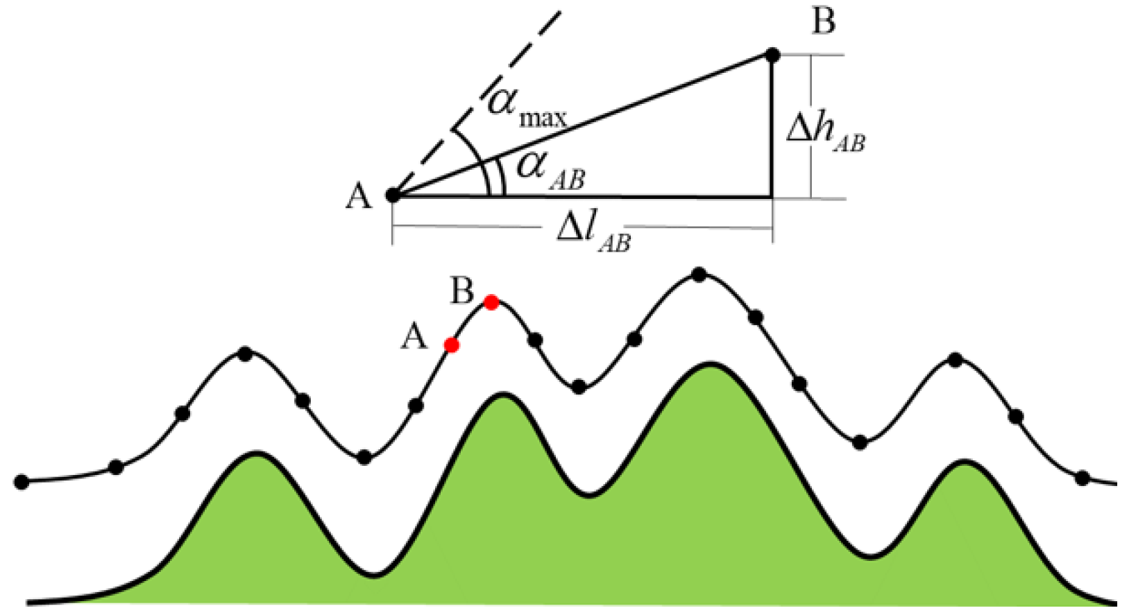
In order to make the planned track match the performance of the fixed-wing aircraft and avoid collision between the aircraft and the mountain obstacles during the landing process, it is necessary to explore the DEM slope calculation method in combination with the pitch angle limit of the fixed-wing aircraft. The slope of DEM is a description of the steepness of the terrain in three-dimensional space. The mathematical model of the slope description is shown as follows:

$$S=\arctan \sqrt{{\phi }_g^2\left(h\right)+{\phi }_t^2\left(h\right)}$$

(9)

Among them, ${\phi }_g\left(h\right)$ and ${\phi }_t\left(h\right)$ are the difference algorithms in the direction of $g$ and $t$. The commonly used numerical analysis methods for slope calculation on DEM mainly include simple difference, second-order difference, third-order inverse distance square weight difference, third-order inverse distance weight difference, third-order unweighted difference, and frame difference. The corresponding ${\phi }_g\left(h\right)$ and ${\phi }_t\left(h\right)$ in the different algorithms above are shown in

Table A2. Comparison table of ${\phi }_g\left(h\right)$ and ${\phi }_t\left(h\right)$ in simple difference, second-order difference, third-order inverse distance square weight difference, third-order inverse distance weight difference, third-order unweighted difference, and frame difference algorithms.

Algorithms	${\mathit{\phi }}_{\mathit{g}}\left(\mathit{h}\right)$	${\mathit{\phi }}_{\mathit{t}}\left(\mathit{h}\right)$
Simple difference	$\frac{h_0-h_4}{{\delta }_g}$	$\frac{h_0-h_2}{{\delta }_t}$
Second-order difference	$\frac{h_4-h_8}{2{\delta }_g}$	$\frac{h_2-h_6}{2{\delta }_t}$
Third-order inverse distance square weight difference	$\frac{h_1-h_3+2\left(h_8-h_4\right)+h_7-h_5}{8{\delta }_g}$	$\frac{h_5-h_3+2\left(h_6-h_2\right)+h_7-h_1}{8{\delta }_t}$
Third-order inverse distance weight difference	$\frac{h_1-h_3+\sqrt{2}\left(h_8-h_4\right)+h_7-h_5}{\left(4+2\sqrt{2}\right){\delta }_g}$	$\frac{h_5-h_3+\sqrt{2}\left(h_6-h_2\right)+h_7-h_1}{\left(4+2\sqrt{2}\right){\delta }_t}$
Third-order unweighted difference	$\frac{h_1-h_3+h_8-h_4+h_7-h_5}{6{\delta }_g}$	$\frac{h_5-h_3+h_6-h_2+h_7-h_1}{6{\delta }_t}$
Frame difference	$\frac{h_1-h_3+h_7-h_5}{4{\delta }_g}$	$\frac{h_5-h_3+h_7-h_1}{4{\delta }_t}$

in the Appendix B. In order to obtain a better slope estimation effect, we use the third-order inverse distance square weight difference algorithm to describe ${\phi }_g\left(h\right)$ and ${\phi }_t\left(h\right)$.

Since the slope calculation result is the slope value represented by the radian, in order to facilitate the cost calculation in the pathfinding algorithm and shorten the storage of the digital map, this paper uses the angle to represent the slope value combined with the pitch angle limit of the aircraft, and converts the angle value into an 8-bit unsigned integer in the range of $\left[0, 2^8-1\right]$, which is shown as follows.

$$G_{g,t}=\left(2^8-1\right)\left(\frac{\frac{\pi }{180}{S}_{g,t}-{\alpha }_{\min }}{{\alpha }_{\max }-{\alpha }_{\min }}\right)$$

(10)

Among them, the maximum and minimum values of the pitch angle of the civil aircraft specified for the task requirements are represented by ${\alpha }_{\max }$, ${\alpha }_{min}$, respectively, and the general minimum value defaults to 0. $G_{g,t}$ can be used as a gray value to store the digital map as gray map data related to the performance of civil aircraft, which supports the cost calculation of the improved A* path planning algorithm.

4. Improved A* Path Planning Algorithm

On the premise of flying close to the ground, if the fixed-wing aircraft can fly along the track with gentle terrain, it can maintain a high speed and the task execution time will be shorter. In order to obtain a smoother and more efficient flight trajectory, an improved A* algorithm based on terrain slope is designed.

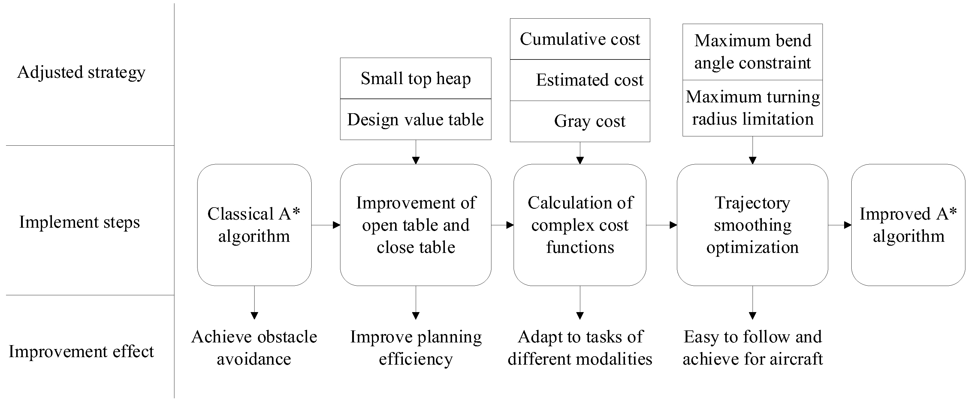
The A* algorithm in the path planning algorithm can quickly find the optimal solution and obtain the shortest path. It is undoubtedly the best algorithm for global path planning in mountainous terrain, but it still has some shortcomings. Aiming at the defects of the classical A* algorithm and the target requirements of real-time global path planning, the optimization steps are shown in Figure 5.

In Figure 5, based on the classical A* algorithm, the data storage and extraction structure in open and close tables is optimized to improve the efficiency of the algorithm. The second part is about the optimization and adjustment of the cost function. The terrain slope parameters are fused into the cost function of the A* algorithm, and different cost functions are calculated according to different requirements to obtain the planned tracks under different task modes. Finally, considering the limitation of aircraft performance, the track is post-processed to generate a three-dimensional safe track after smoothing the height and turning angle, so that the track is easy to follow.

4.1. Cost Function Optimization

Compared with the classical A* algorithm, the cost function $F_n$ is adjusted by Equation (11).

$$F_n(G_n,H_n,I_n)={\omega }_G{G}_n+{\omega }_H{H}_n+{\omega }_I{I}_n$$

(11)

Among them,$G_n$ is the sum of the cost from the starting point $B_{g,t}$ to the current point $x_n$, the cost that needs to be spent from the current point to the end point is expressed as $H_n$, the cost of the newly added gray value is expressed as $I_n$, ${\omega }_H$ is the weight of the estimated distance cost, ${\omega }_I$ is the weight of the slope cost, and ${\omega }_G$ is the weight of the distance cost that has been spent. The calculation method of $G_n$ can be adjusted by the grid distance in different directions, and the distance calculation method of $H_n$can be adjusted according to the actual model of DEM. The calculation process of the optimized cost function is shown in Algorithm A1.

4.1.1. Cumulative Cost

The grid in the DEM is not a standard rectangle, and the grid length deformation after the Gaussian model projection is worse. Therefore, different weights need to be added to the distance in the latitude and longitude directions. However, due to the different weights of different longitudes and latitudes, there will be a large amount of calculation. Therefore, in order to take the calculation accuracy and calculation efficiency into account, the deformation within the same longitude and latitude is regarded as the same, so the distance calculation is adjusted to the following formula:

$$\left\{\begin{array}{l}{\delta }_g=\frac{L_t}{N}\cos \left(\left[t\right]\right)\\ {\delta }_t=\frac{L_t}{N}\end{array}\right.$$

(12)

Among them, $L_t$ is the actual distance of a latitude range, $N$ refers to the number of grids per unit latitude or unit longitude range, $\left[t\right]$ is the latitude value rounded, and ${\delta }_g$ and ${\delta }_t$ are the actual distance of a single grid in the longitude and latitude directions.

According to the distance calculation formula and the extended node method of the eight neighborhoods in the A* algorithm, the calculation formula of the cumulative cost $G_n$ can be described as following formula:

$$G_n=G_{n-1}+\frac{L_t}{N}\left\{\begin{array}{l}\cos \left(\left[t\right]\right)\hspace{1em}\hspace{1em}\hspace{1em}{n}_j=4,8\\ 1\hspace{1em}\hspace{1em}\hspace{1em}\hspace{1em}\hspace{1em} n_j=2,6\\ \sqrt{{\cos }^2\left(\left[t\right]\right)+1} n_j=1,3,5,7\end{array}\right.$$

(13)

Among them, $n_j$ is the eight neighborhoods index of the parent node relative to the current node, and $G_{n-1}$ is the cumulative cost of the previous node. The different positions of the previous node in the eight neighborhoods will change the cost from the previous node to the current node. Since $L_t$, $\left[t\right]$, and $N$ are constant values, the cumulative cost will also be a constant value in the same latitude map with the same resolution. The cumulative cost change generated by a single expansion will change due to the difference in the position $j$ of the extended node relative to the current node.

4.1.2. Estimated Cost

The estimated cost $H_n$ is the cost of estimating the current point to the target point, which can be calculated by the Manhattan distance algorithm with modified latitude and longitude difference.

$$\left\{\begin{array}{l}{H}_n=\Delta g_{n,E}+\Delta t_{n,E}\\ \Delta g_{n,E}=\frac{\cos \left(\left[t\right]\right)N_t}{N_g}\left|g_n-g_E\right|\\ \Delta t_{n,E}=\left|t_n-t_E\right|\end{array}\right.$$

(14)

Among them, the distance length in the direction g and the error value in the direction $t$ will also be calculated into the distance difference $\mathsf{\Delta }{g}_{n,E}$ in the $g$ direction, so as to synchronize with $G_n$ to eliminate the influence of Gaussian projection on the grid distance deformation.

4.1.3. Gray Cost

The gray cost $I_n$ is the cost of the influence of the terrain slope on the flight of the aircraft. Because it is difficult for the aircraft to climb at a high speed when flying near the ground, it is necessary to limit the terrain slope to find a safe and fast trajectory that can satisfy the pitch angle limit of the aircraft at a certain speed. Taking the gray cost as a part of the cost function in the pathfinding algorithm, the calculation method is the same as the method of gray value as follows:

$$I_n=\left(2^8-1\right)\left(\frac{\frac{\pi }{180}{S}_{g,t}-{\alpha }_{\min }}{{\alpha }_{\max }-{\alpha }_{\min }}\right)$$

(15)

4.2. Optimization of Open Table and Close Table

During the execution of the A* algorithm, it is necessary to continuously add selected nodes to the close table, and continuously insert new nodes, delete root nodes, and modify existing nodes in the open table. The classical A* algorithm uses an array structure, and all points that may be traversed are placed in an array of the same open table, and sorted according to different costs.

The purpose of sorting the open table is to always be able to locate the minimum cost point, and to facilitate the insertion of new nodes, modify existing nodes, and delete the minimum point for operation. Therefore, the data structure of the close table and the open table greatly affects the traversal and search efficiency of the nodes.

This paper explores the efficient array sorting method and proposes the following improvement schemes:

(1)

An improved data structure “value table” is designed, which combines the open table and the close table. It avoids the heuristic search operation on the array matrix before sorting the open table in the classical A* algorithm, which must have to judge whether the points in the eight fields have appeared in the open table or the close table.

(2)

Using “Small Top Heap” to efficiently sort the nodes in the value table when performing operations such as inserting new nodes, deleting root nodes, and modifying nodes, to ensure that the root node in each extracted sequence is the minimum value, and the cost function gradually increases from the root node to the child node. The time complexity is $O\left(n\mathit{log}n\right)$ and the space complexity is $O\left(1\right)$, which is lower than other sorting algorithms.

The following will describe the details of the value table designed to improve the search efficiency and the operation details of inserting new nodes, deleting root nodes, and modifying nodes in the value table by using the Heap sort order to improve the sorting efficiency.

4.2.1. Value Table

The information of the points stored in the traditional open table is two-dimensional coordinates. The new value table is stacked by rows and then the minimum points are stacked by columns. This sorting method can be stored for different rows, and only the column coordinates of the corresponding rows need to be stored. In the final value table, only the column coordinate index, the proxy value, and the parent node index that the original open table should store are retained. At the same time, because the parent node of the current point must be a point in the eight-neighborhood, the index of the parent node can replace the original two-dimensional coordinate index by the serial number of the eight-neighborhood. The close table stores two-dimensional coordinates and parent nodes, which are repeated with the open table, so the open table and the close table are merged. Because the open table does not calculate the nodes in the close table into the array when sorting, the value in the close table is set to a null value.

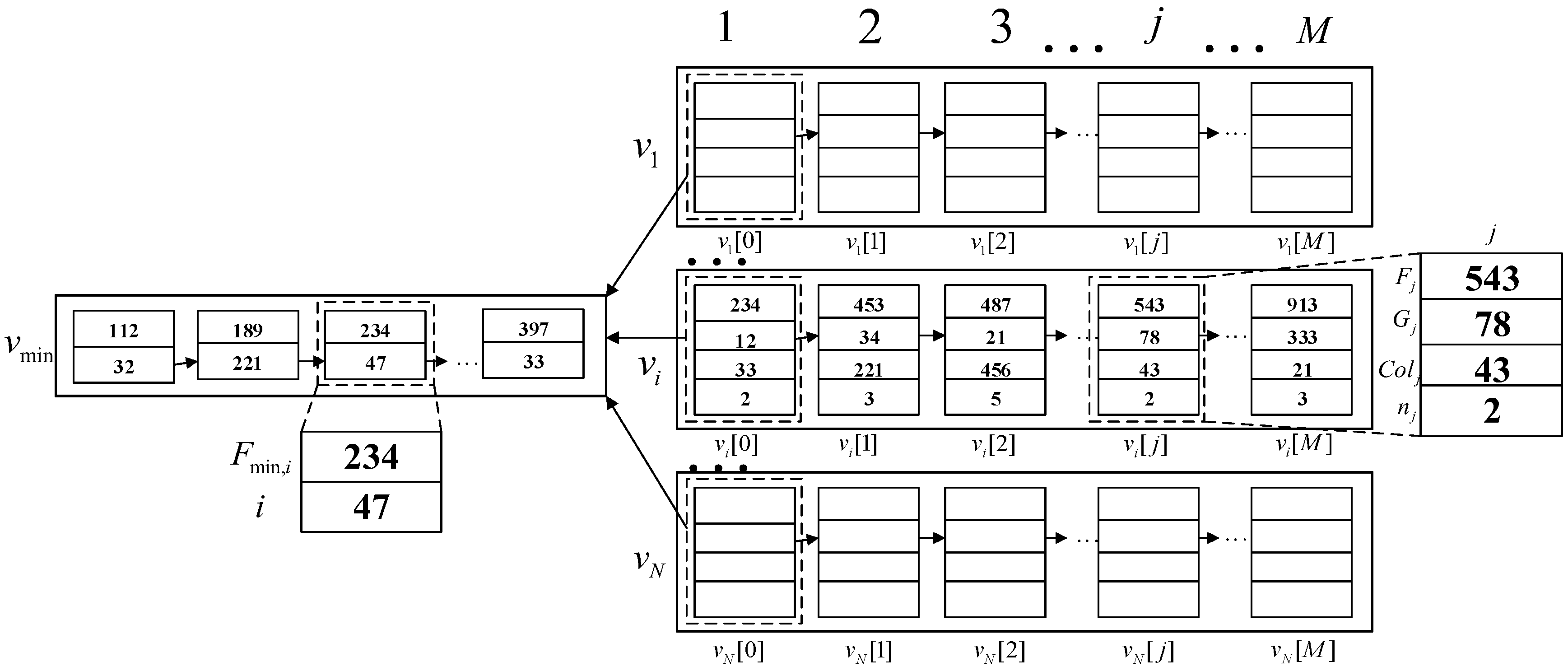
The “value table” proposed in this article combines the open table and the close table, and its data structure is shown in Figure 6.

The value table contains $N$ arrays of $v_i$ rows, and a row array of minimum cost $v_{\min }$. Row array $v_i$ contains cost value $F_j$, cumulative cost $G_j$, the column index $co{l}_j$ of current point $j$, and the index $n_j$ of the eight neighborhoods parent node. The minimum cost array $v_{\min }$ contains the cost value $F_{\min ,i}$ minimum value in $v_i$, and its row index $i$, among which $N$ is the row numbers of DEM, and $M$ is the column number of DEM.

When it comes to the situation that the parameter $(F_i,G_i,n_i)$ of node $(g_i,t_i)$ needs to be updated, the column index $j$ in row array $v_i$ should be retrieved at first where index $j$ can perfectly match $t_i$. The row array $v_i$ will be automatically sorted in ascending order by the Heap sorting method. Specific details will be shown in Algorithm A2.

Table $v_{\min }$ stores the cost values and row index of every root node $v_i\left[0\right]$ for all $(v_1,v_2,...v_N)$. When the root node value $v_i\left[0\right]$ of $v_i$ is modified, the $v_{\min }\left[k\right]$ matched to the index $i$ ($v_{\min \left[k\right]}.i=i$) and $v_{\min \left[k\right]}.F_{\min ,i}$ will also be modified later. The row array $v_{\min }$ will be automatically sorted by $F_{\min ,i}$ ascending order by the Heap sorting method. Specific details will be shown in Algorithm A3.

According to the continuously backtracking operation of index $v_{\min }\left[0\right].i$ in $\left(v_1\right[0].n,v_2[0].n,...v_N[0].n)$ after getting the final $v_{\min }$, the row index $g_i$ of the target point will be reached. The column $t_i$ of the target point in $\left(v_1\right[0].col,v_2[0].col,...v_N[0].col)$ will be reached by continuously backtracking operation at the same time. Specific details will be shown in Algorithm A4.

The parent node of the current node must belong to one of the eight neighbor nodes of the current node in the improved A* algorithm, based on which the information of the parent node can be gotten by the eight neighbors index relative to the current node, for which the backtracking operation is feasible.

4.2.2. Heap Sorting Method

(1)

Inserting new nodes

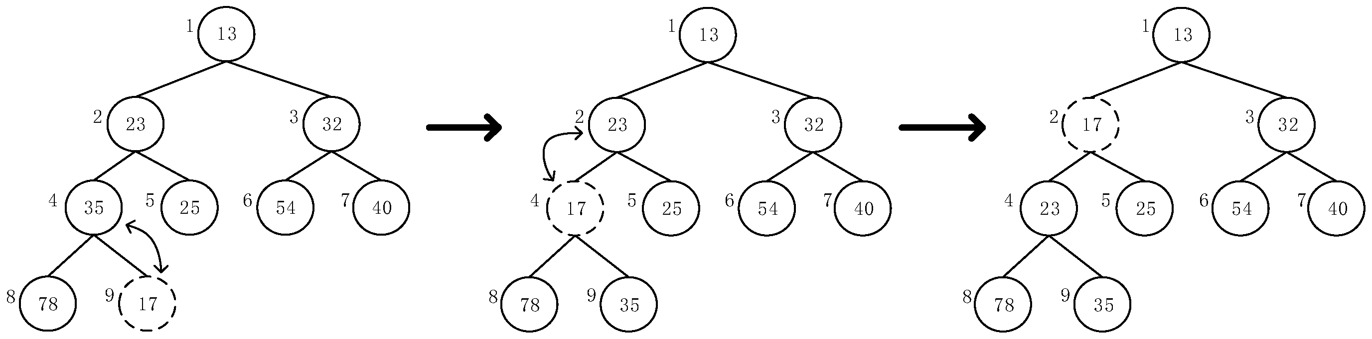
The diagram of inserting new nodes is shown in Figure 7. Firstly, the new node is placed at the end of the array (node 9 in the graph), and then the size of the new node and the parent node are compared (node 4 and node 9 in the graph). If the new node is smaller than the parent node, the new node is exchanged with the parent node. Repeat the comparison and exchange until the parent node is less than the new node. The process of inserting a new node is the process by which the node continues to rise from the end of the binary tree.

(2)

Deleting root nodes

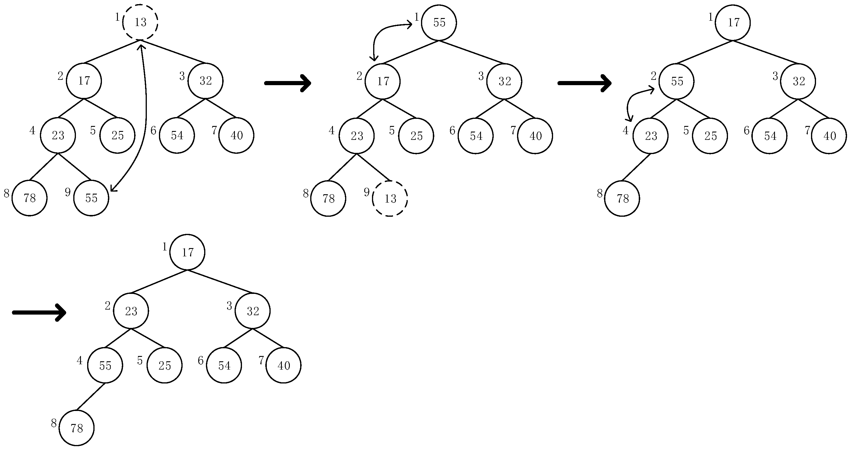
The schematic diagram of deleting root nodes is shown in Figure 8. Firstly, the root node and the end node are exchanged (node 1 and node 9 in Figure 8). At this time, the original root node (node 9) can be deleted, and the new root node is the original end node. The new root node is compared with the child node and exchanged with the smaller node in the child node; that is, node 1 and node 2 are exchanged in the graph until the child node is larger than this node. The process of deleting new nodes is the process of continuous sinking down of nodes from the root nodes of the binary tree.

(3)

Modifying nodes

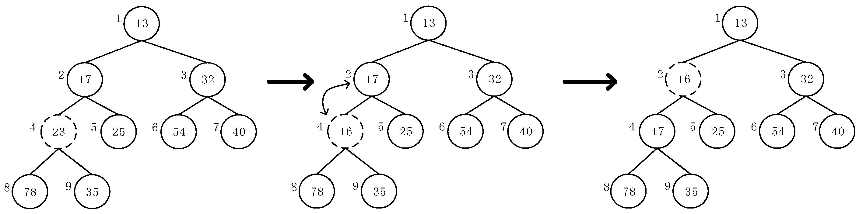
The schematic diagram of modifying the node is shown in Figure 9. The value of the node is modified to the changed value. Owing to the reason that the modification of the node in the value table reduces the node value, the process of modifying the node is the process of the node floating up, which is the same as the process of inserting new nodes.

4.3. Trajectory Smoothing Optimization

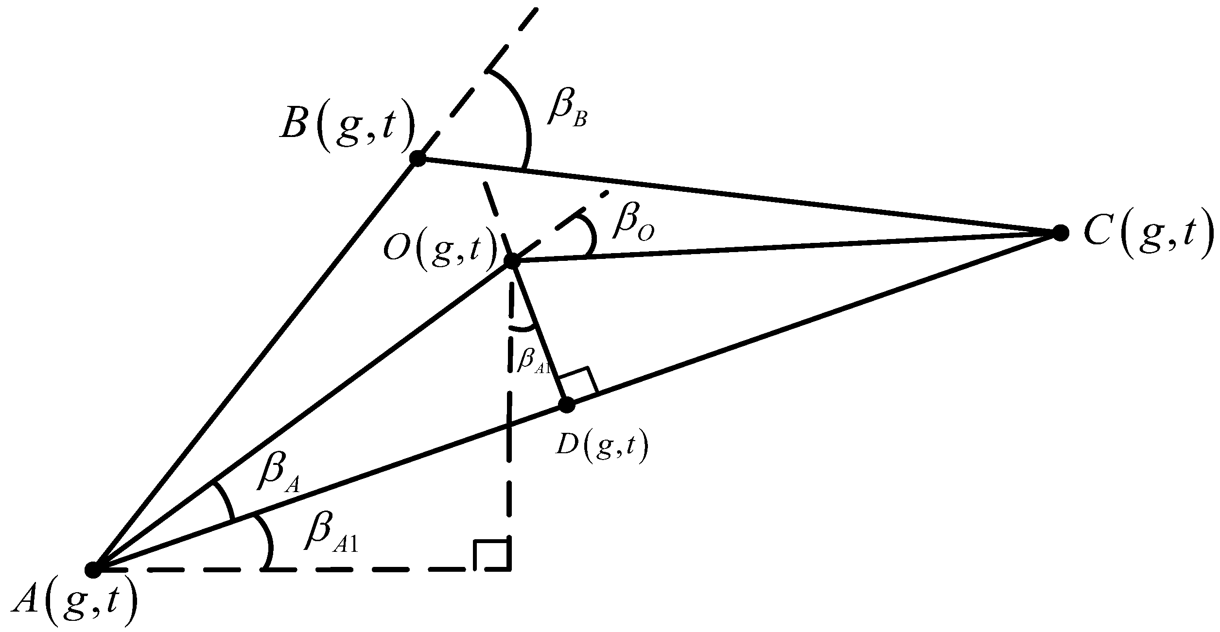
While the coordinates of the eight neighborhoods are used in the path planning process with constant angle of path, the turning radius of the aircraft in the actual flight is limited. For the convenience of calculation, the maximum turning angle between the three waypoints is limited on the basis of the step size of about 200 m, so that the route can meet the performance requirements of the aircraft. Aiming at the processing of the turning angle, this paper designs the vertical line method to adjust the trajectory, as shown in Figure 10.

For the continuous track points $A$, $B$, and $C$, the turning angle at the track point $B$ is ${\beta }_B$. When ${\beta }_B>{\beta }_{\max }$, it is necessary to find a point $O\left(g,t\right)$ so that ${\beta }_O$ can meet the constraint of ${\beta }_O\le {\beta }_{\max }$. In order to make the step size between the two track points as consistent as possible, this paper is designed to find point $O$ on the vertical line of $AC$, and its corresponding relationship is:

$${\beta }_O=2{\beta }_A=2\arctan \left(\frac{OD}{\frac{1}{2}AC}\right)={\beta }_{\max }$$

(16)

Through the above equation, the quantitative relationship between $OD$ and the coordinates of $A$ and $C$ can be obtained as follows:

$$OD=AD\tan \left({\beta }_A\right)=\frac{\sqrt{{\left(g_C-g_A\right)}^2+{\left(t_C-t_A\right)}^2}}{2}\tan \left(\frac{{\beta }_{\max }}{2}\right)$$

(17)

The coordinate $O$ can be obtained according to the midpoint $D$ between coordinate $A$ and the midpoint of coordinate $C$, line segment $OD$, and the coordinate axis angle ${\beta }_{A1}$ as follows:

$$\left\{\begin{array}{l}{\beta }_{A1}=\arctan \left(\left|\frac{g_C-g_A}{t_C-t_A}\right|\right)\\ g_D=\frac{g_C+g_A}{2}\\ t_D=\frac{t_C+t_A}{2}\end{array}\right.\Rightarrow \left\{\begin{array}{l}{g}_O=g_D+OD\frac{g_B-g_D}{\left|g_B-g_D\right|}\sin {\beta }_{A1}\\ t_O=t_D+OD\frac{t_B-t_D}{\left|t_B-t_D\right|}\cos {\beta }_{A1}\end{array}\right.$$

(18)

The trajectory after optimization is smoother; it can better meet the constraint of the turning angle of the aircraft. The pseudo-code of the improved A* algorithm is described in Algorithm A5.

5. Results

5.1. Experimental Environment

The hardware environment of the laboratory uses an 8-core,16-thread Intel I3-10th-2.4 GHZ main frequency processor, 4G running memory, and GeForce GTX 750 graphics card.

5.2. Experimental Parameters

The test parameters designed for specific global path planning tasks are shown in

Table 1. Algorithm simulation default parameter table.

Parameter	Value	Parameter	Value
Longitude of starting point	109.790833°	Longitude of target point	109.371667°
Latitude of starting point	36.718333°	Latitude of target point	36.091667°
Gray image minimum slope	0°	Minimum path segment length	200 m
Gray image maximum slope	30°	Interpolation algorithm	2D cubic convolution
Minimum terrain clearance altitude	800 m	Difference algorithm	Third-order inverse distance Squared weight difference
Maximum terrain clearance altitude	12,600 m	Distance type	Manhattan distance
Minimum pitch angle	0°	Cost weight of G	0.6
Maximum pitch angle	10°	Cost weight of H	0.2
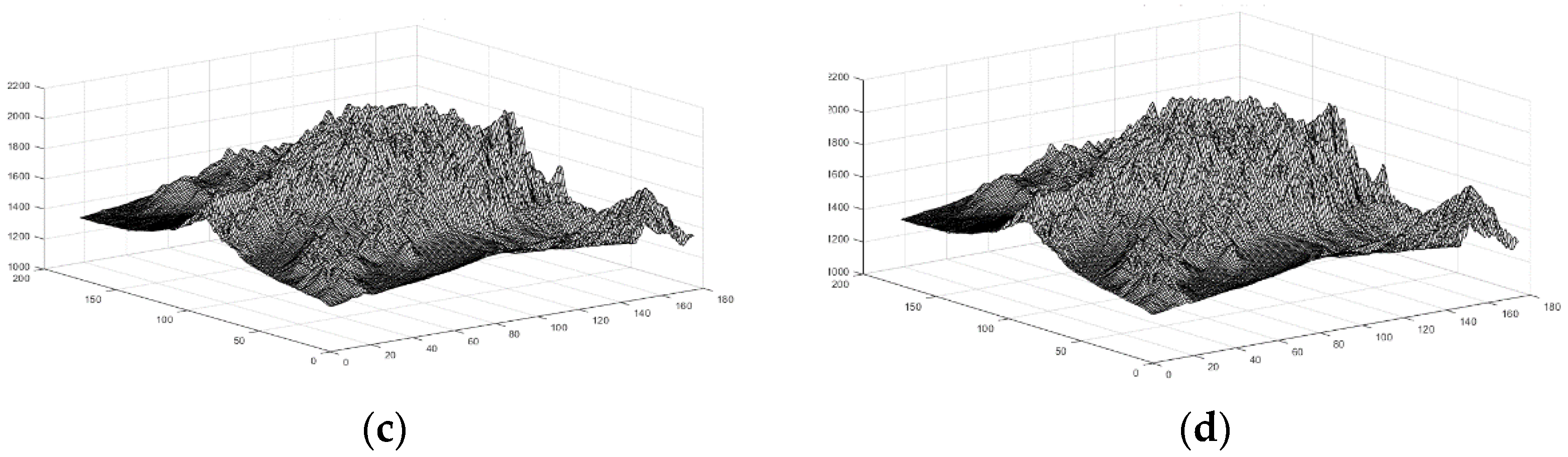
Maximum turning angle	10°	Cost weight of I	0.2

. The default starting point and the target point are located in the DEM range of N36E109~N37E110, the DEM resolution is 90 m, the number of grids in the longitude direction and latitude direction is 1201, the projection is Gaussian projection, and the coordinate system is the WGS-84 coordinate system. The terrain top view rendering map and three-dimensional map are shown in Figure 11.

5.3. Experimental Results and Analysis

In this paper, the classical A* algorithm and the improved A* algorithm are run separately, the planning parameters of different algorithms are counted, and the classical algorithms and the improved algorithms are compared from the aspects of planning effect and efficiency as

Table 2. Comparison simulation data of algorithm before and after improvement.

Simulation Data	Classical A* Algorithm	Improved A* Algorithm
Map processing time/s	0.0669	0.4220
Path planning time/s	412.6251	4.4212
Length of trajectory/m	93,620	93,225

.

Through the comparison data of the simulation results in Table 2, it can be seen that the improved A* algorithm has increased the map processing time compared with the traditional algorithm, which is due to the increase in map resolution adjustment and slope calculation in the early stage. Such time consumption is necessary, because the processing of the map facilitates the subsequent pathfinding algorithm, and the length of trajectory becomes smaller. It can be seen that in the results, the pathfinding time of the improved algorithm is 1% of the traditional algorithm, and the time is greatly shortened. Finally, the length of the track planned by the improved algorithm is also shorter than that of the traditional algorithm. Although the shortened length is not much for the whole track, it also saves the time to reach the target point to a certain extent.

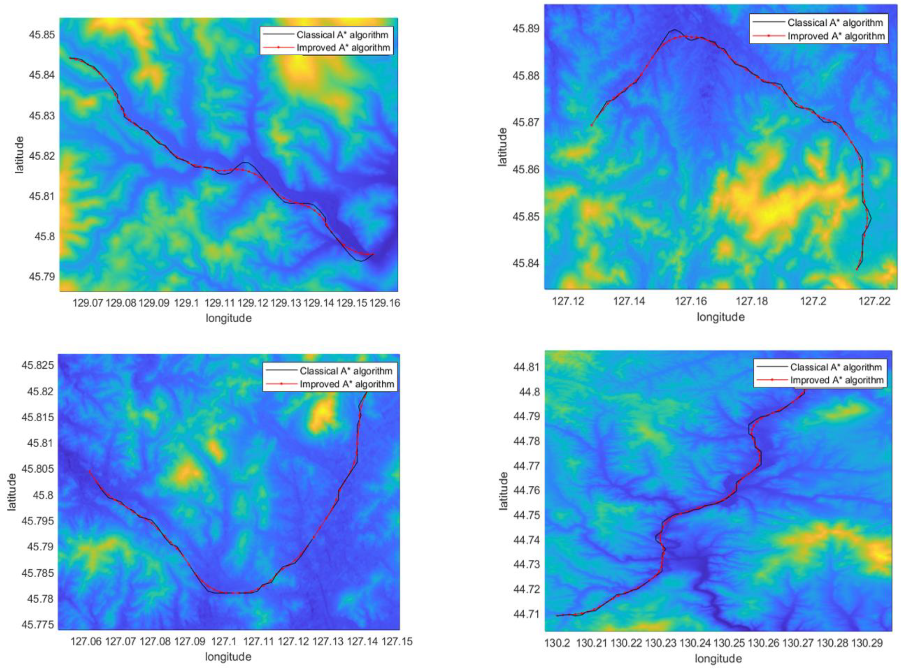
Combined with the planning path in the schematic diagram of the algorithm simulation performance results between the classical algorithm and the improved algorithm in Figure 12, the point line is the classical A* algorithm, and the solid line is the improved A* algorithm. It can be seen that the path planned by the improved A* algorithm has less steering. In a valley with complex terrain, the path can also be adjusted according to the change in valley terrain to satisfy the constraint of obstacle avoidance.

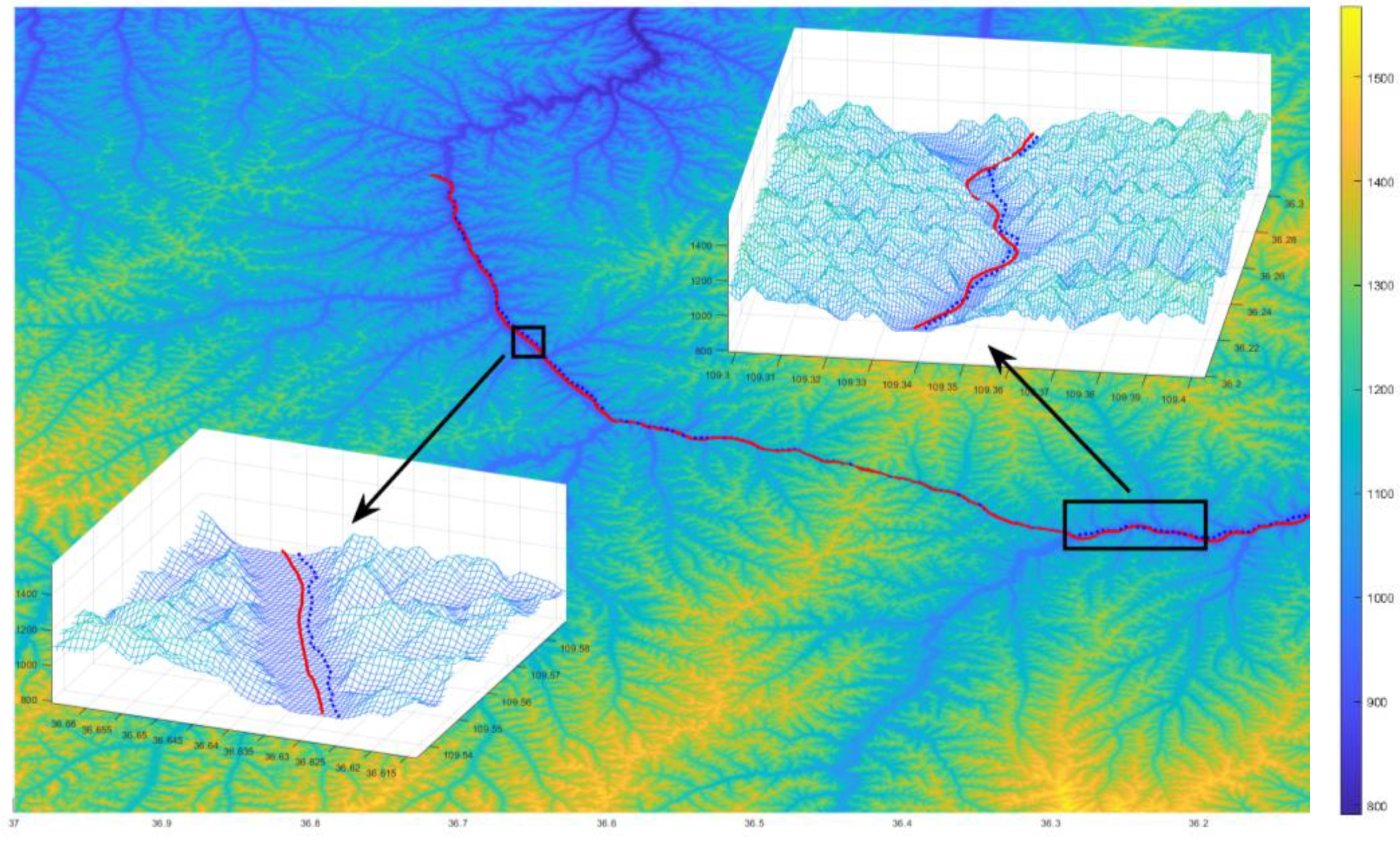
When the aircraft makes an emergency landing in a complex mountain flight, the flight trajectory after trajectory smoothing optimization shows a smoother landing route with shorter track distance and landing time, as shown in Figure 13. Therefore, the improved A* algorithm improves a good solution for the emergency handling of fixed-wing aircraft in the event of bad weather conditions.

5.4. Comparative Analysis

In the previous study, the interpolation algorithm was introduced and the 2D cubic convolution interpolation selected as the best interpolation algorithm by comparing the effect of interpolation maps. In order to verify the superiority of 2D cubic convolution interpolation, this section will simulate different interpolation algorithms. The DEM obtained by different algorithms is used to find the path, and the parameters such as the pathfinding time and the path length of the path planned by different algorithms are compared. For the task requirements of different minimum track segment lengths, this paper designs four digital maps with different resolutions to meet the requirements of interpolation algorithms under different task situations.

The minimum track length of the contrast experiment design of the interpolation algorithm is 30 m, 45 m, 200 m, and 500 m for the four groups of algorithm simulation. The simulation results are shown in

Table 3. Comparison simulation data of different minimum track length and interpolation algorithm.

Minimum Track Length	Simulation Data	Bilinear	Bicubic Hermite	2D Cubic Convolution
30 m	Map processing time/s	51.15	84.83	38.04
	Path planning time/s	1614.14	1618.77	1859.43
	Length of trajectory/m	97,509	98,486	98,486
45 m	Map processing time/s	29.54	53.12	17.51
	Path planning time/s	831.19	784.20	742.94
	Length of trajectory/m	97,029	97,095	97,095
200 m	Map processing time/s	1.47	2.52	0.61
	Path planning time/s	7.06	7.80	7.91
	Length of trajectory/m	93,879	93,241	93,241
500 m	Map processing time/s	0.20	0.31	0.08
	Path planning time/s	0.64	0.61	0.60
	Length of trajectory/m	83,156	84,039	84,039

.

Through the setting of different minimum track segment lengths, it can be seen that when the gray image obtained by the interpolation algorithm is used for pathfinding, the map processing time of the two-dimensional cubic convolution interpolation algorithm is the smallest, followed by the two-dimensional cubic convolution interpolation, and the map processing time required for the bicubic Hermite interpolation is the longest. The three interpolation algorithms have little difference in pathfinding time under different resolutions, and most of the pathfinding time of the bicubic Hermite interpolation is relatively small; the effect of bilinear interpolation will become relatively poor as the resolution decreases, while the bicubic Hermite interpolation and the two-dimensional cubic convolution interpolation are consistent with the track length data.

By longitudinally comparing the simulation parameters obtained by the same interpolation algorithm with different resolutions, it can be seen that the higher the resolution, the less time spent on the map processing and pathfinding algorithm of the response. When the pilot actually flies, the resolution can be adjusted as needed to improve the efficiency of the algorithm. The 2D cubic convolution method can also obtain a trajectory with higher accuracy.

In the previous section, by comparing the slope calculation effect and calculation complexity of different algorithms, the third-order inverse distance square weight difference method is selected as the slope calculation method of track planning. In order to further determine its superiority, this section will simulate and test the DEM obtained by different difference algorithms, and compare the pathfinding effect of different difference algorithms. The difference algorithm simulation data comparison is shown in

Table 4. Comparison simulation data of different difference algorithms.

Difference Algorithm	Map Processing Time/s	Path Planning Time/s	Length of Trajectory/m
Simple difference	0.40	4.18	93,314
Second-order difference	0.39	4.92	93,319
Third-order inverse distance square weight difference	0.41	4.84	93,241
Third-order inverse distance weight difference	0.40	4.67	94,238
Third-order unweighted difference	0.39	4.86	94,183
Frame difference	0.40	4.54	94,352

.

It can be seen from the simulation data that the map processing times and pathfinding times of different differential algorithms are less different, so the selection of different difference algorithms has little effect on the final performance.

In the previous section, by comparing the computational efficiency and accuracy of different distance calculation methods, the Manhattan distance is selected as the distance calculation method in the path planning. Because the latitude and longitude distances in the grid are different, the latitude and longitude distance difference are combined with the Manhattan distance.

In this section, in order to compare the effects of different distance calculation methods for path planning, we randomly generate 1000 groups of starting points and target points in the same map. We define the minimum pathfinding time (MPFT) to measure the number of minimum pathfinding algorithms for an algorithm in 1000 path plans as shown in Equation (19).

$$MPF{T}_i={\displaystyle \sum }_{k=1}^{1000}1[i==\underset{1\le j\le 4}{\arg \min }\{t_j^{(k)}\}],i=1,2,3,4$$

(19)

where $t_1^{\left(k\right)},t_2^{\left(k\right)},t_3^{\left(k\right)},t_4^{\left(k\right)}$ represent the path planning time under the Euclidean distance, Manhattan distance, Diagonal distance, and Chebyshev distance, respectively, in $k$-th simulation. $1\left(x\right)$ is an indicative function when $x$ is true; its value is 1, otherwise it is 0. Comparison simulation data of different distance calculation methods in $MPFT$ are shown in

Table 5. Comparison simulation data of different distance calculation methods in MPFT.

Euclidean Distance	Manhattan Distance	Diagonal Distance	Chebyshev Distance
128	613	19	240

.

According to the statistical results, it can be seen that among the 1000 groups of random tracks, the Manhattan distance has the shortest pathfinding time of 613 times. Therefore, it is undoubtedly the best distance calculation method in the pathfinding algorithm.

6. Discussion

The path planning method based on the improved A* algorithm proposed in this paper has significant advantages compared with the classical A* algorithm. Take the original A* algorithm (including A* [4], LPA* [27], Weighted A* [28,29], etc.) and Hybrid A* algorithm [27] as an example; their characteristics are shown in

Table 6. Comparison of different A* algorithms.

Algorithm	Processed Map Format	Sorting Algorithm of Node Data	Storage Structure of Node Data	Smooth Optimization Method of Trajectory
Original A*	Digital raster Graphics (DRG)	Insertion sorting or other sorting methods	Open table and close table	No optimization
Hybrid A*				Consider kinematic corner constraints, using Dubbins curves, or Reeds Shepp curves for trajectory smoothing
Improved A*	DEM after preprocessing of map	Small Top Heap sorting	Value table	Consider turning angle constraint real-time midline optimization

.

Through the preprocessing operation of resolution adjustment and interpolation of DEM map information, a “value table” is used to store open table node data, and the Small Top Heap structure is used to delete, add, modify, and sort nodes, which greatly reduces the calculation time. The turning angle of the two-dimensional trajectory point calculated by the A* algorithm is smoothed to ensure the planned trajectory point meets the requirements of the aircraft turning angle.

The simulation examples show that the proposed improved A* algorithm can meet the requirements of short calculation time, good smoothness of calculation trajectory, and high security. However, the current trajectory planning algorithm does not consider the underlying dynamic model of the aircraft and the requirements of control performance. In future research, it is planned to incorporate the influence of aircraft speed into the algorithm; that is, the maximum and minimum flight speed effects of the aircraft are considered in the process of planning the trajectory, so that the planned trajectory can meet the flight speed constraints of the aircraft. In addition, the weight distribution of the generation value in the improved A* algorithm and the efficient real-time re-planning obstacle avoidance in the dynamic environment are also problems worthy of further study.

7. Conclusions

This article takes the FMS system of fixed-wing civil aircraft as the background for efficient emergency landing obstacle avoidance and optimal trajectory planning in complex mountainous terrain. It mainly focuses on model generation and preprocessing in global path planning, as well as global path planning algorithms.

This article uses methods such as adjusting map resolution, calculating terrain slope, and generating safe flight surface to preprocess map information, and generates a flyable DEM grayscale map. This solves the problem of excessive data volume in the three-dimensional spatial model of the trajectory planning algorithm, and based on this, generates the grayscale cost of the path planning algorithm. A global path planning algorithm based on the improved A* algorithm combined with grayscale cost is proposed, the effectiveness of the final experimental results of the algorithm is analyzed, and the key interpolation and heuristic operator calculation methods that affect the algorithm are compared and analyzed.

The overall work of the paper is as follows:

A safe flight surface generation algorithm combining pitch angle constraint is proposed to meet the requirements of pathfinding algorithms for digital maps. Select DEM as the data model for the three-dimensional spatial model, and perform two-dimensional cubic convolutional interpolation to address the resolution issue of the digital map, resulting in a digital map that can meet the storage requirements of the pathfinding algorithm and the safety of flight surface information. To address the issue of large amounts of elevation data that are difficult to calculate, a third-order inverse distance squared difference method is used to calculate the terrain slope and generate a grayscale image.

A global path planning algorithm based on the improved A* algorithm is proposed to solve the problems of low planning efficiency and difficulty in following the trajectory. To solve the problems of large data computation and long planning time in the classical A* algorithm, value table and Small Top Heap methods are used to improve and optimize the sorting algorithm and data structure; a trajectory smoothing optimization algorithm combined with turning angle constraints is proposed to address the problem of difficult track following. And comparative analysis of key methods is conducted on the optimized algorithm.

The experimental results show that, compared to the original classic A* algorithm, the improved A* algorithm can significantly reduce the pathfinding time of the flight path, and the planned flight path is smoother and easier to follow, which meets well the requirements of efficient obstacle avoidance and emergency landing in complex mountainous terrain.