A Digital Twin-Based Approach for the Optimization of Floor-Ball Manufacturing

Abstract

The increasing complexity of products and manufacturing processes, combined with the constantly advancing technological integration of the manufacturing sector, raised new challenges for world-class industries to optimize time-to-market, resources, and cost. Simulation, as an essential Industry 4.0 enabling technology, allows one to emulate the steps of a manufacturing process, thereby achieving significant improvements in all the product and process development phases. A simulation process can be implemented and improved by creating the Digital Twin of the manufacturing system, which can be realized on a single-line scale or extended to the whole factory. The Digital Twin merges physics-based system modeling and real-time process data to generate a virtual copy of an observable object to reduce and optimize the extensive time and cost of physical design, prototyping, commissioning, reconfiguration, and maintenance. This study aims to investigate how the implementation of digital twin technology can help optimize the balance between power consumption and productivity, taking into account existing barriers and limitations. By following this outline, this study shows the design and development of a digital twin for a floor-ball manufacturing line present in the Smart Factory of Ostschweizer Fachhochschule (Switzerland). The entire production process is reproduced with Siemens Technomatix Plant Simulation software 2201, and data connection and processing are handled by a tailored toolchain consisting of an agent, a database, Python packages, and the COM interface from Tecnomatix. This toolchain feeds the digital twin with data from the physical operating environment. In particular, this study compares direct power measurements with the ones expected by the digital twin to assess digital model accuracy.

1. Introduction

The recent development of the Industry 4.0 concept [1] and the increased performance with reduced costs for big data analytics [2], fostered by faster algorithms, increased computation power, and a more significant amount of available data, enable the real-time simulation, control, and optimization of products and production lines, which is referred to as a Digital Twin (DT) [3,4]. DT was first defined in 2011 by NASA [5] as “an integrated multi-physics, multi-scale, probabilistic simulation of a vehicle or system that uses the best available physical, models, sensor updates, fleet history, and so forth, to mirror the life of its flying twin.” In the context of manufacturing, the DT definition has evolved into the broader and standardized concept of “a digital representation of an observable manufacturing element with synchronization between the element and its digital representation” [6]. The unique combination of digital representation and synchronization between digital copy and real element allows a DT to detect anomalies in manufacturing processes, thus achieving functional objectives such as real-time control, predictive maintenance, in-process adaptation, Big Data analytics, and machine learning. A DT can monitor the related observable manufacturing element by constantly selecting and updating the operational and environmental data. The visibility into process and execution enabled by a DT enhances manufacturing operation and business cooperation, potentially involving the entire manufacturing supply chain up to the final end-users.

DT development requires three main components: (i) an information model, (ii) a communication mechanism, and (iii) a data processing module [3]. Different information sources must be connected to create a DT, and data must be acquired. These data are processed using calculation algorithms and simulation models to represent the observable manufacturing elements, and the whole process is as detailed as possible. Moreover, the information model should be able to generate the DT automatically and in parallel to the real element operation. The information model abstracts the specifications of a physical object and is usually based on standards [7]. The communication mechanism transfers bi-directional data between the DT and the observable counterpart. Changes in the physical object state are detected by sensors and transmitted to the DT in cyberspace. Industrial communication protocols and connectivity play a crucial role. Existing industrial networks are typically implemented with heterogeneous networks, including the three main categories of so-called “Fieldbus” networks [8], Ethernet-based protocols [9], and Internet of Things (IoTs) [10], which typically use wireless networks. The data processing module extracts information from multi-source data to build the virtual representation of the observable object. A complex system has many equipment parameters and significant data redundancy, and these parameters have strong coupling, non-linearity, and time variability, which directly affect data quality. DT uses various data processing technologies and decision support tools such as big data to store, screen, process, and interact with data in real time to judge and process changes in the external environment effectively.

Worldwide technology leaders’ initiatives have pushed the existing market for engineering applications. For example, GE developed a DT platform called PREDIX that can understand and predict asset performance [11]; Siemens covers smart operations during the complete process of design, production, and operation [12]; ABB focuses on enabling data-driven decision-making [13], while Microsoft provides an IoT platform for modeling and analyzing the interactions between people, spaces, and devices [14]. The development of industrial solutions is accompanied by academic research, with a growing outcome in recent years [15]. Some practical applications have already been developed and reported in the literature, including reviews of DT applications in manufacturing. Cimino et al. [16] analyzed and classified 52 articles reporting DT applications in industrial or laboratory manufacturing environments for application purposes, system features, DT implementation features, and DT services. The authors found two significant gaps: the need for DT integration with the control system and the limitation of the set of services offered by the DT. Lu et al. [3] underlined how, compared with the total number of publications on the DT topic, most existing research is conceptual, and only 28 articles reporting practical applications of DT were considered. The authors identified seven key research issues: the DT architecture pattern (server-based vs. edge-based), the communication latency requirement, the data capture mechanism, the need for standard development, limited DT functionalities, the management of DT model versions, and how to include humans in DT applications. Onaji et al. [17] reviewed the DT definition in detail and analyzed three DT case studies. The authors identified seven technical limitations hampering the implementation of DT in manufacturing: the quantification of DT model uncertainties, the virtual confidence, the variance of the communication frameworks, the lack of an explicitly defined ontology, the inclusion of human functionality in the virtual space, the need for professional skills, and the integration into a single platform of different DT subsystems and functions. Nevertheless, all authors from [3,16,17] agreed that since the development of practical DT applications is still at an early stage, it is essential to integrate the existing literature with new case studies, highlighting the limitations and barriers that DT implementation can face in industries and, more specifically, in small-medium enterprises (SMEs).

In parallel with this technological development, optimizing power consumption in manufacturing systems has increased attention in recent years. In particular, climate responsibility and imminent energy shortage have fostered the discussion. Several studies show evidence of the negative impact of power shortage on firm performance for both large and medium-sized companies [18,19]. The DT application has already addressed the topic of energy efficiency in manufacturing. Taisch et al. [20] highlighted the opportunity of using discrete-event simulation with material flow simulation as a standard tool in manufacturing and enriched it by considering energy consumption. The approach was based on the production states of the production assets and showed that implementing energy measures is possible and can lead to a widened decision sense. Mousavi et al. [21] developed an integrated conceptual framework to model the energy consumption of a production system. They demonstrated the ability to obtain practical comprehension of potential energy efficiency improvements through experimentations. Karanjkar et al. [22] presented a case study for deploying an IoT framework in an assembly line where multiple sensors were installed for measuring machine-wise activity and energy consumption profiles. They built a data aggregation platform and a discrete-event DT of the line by using open-source tools. These sensors’ data were collected at a high sampling rate, but the machine state estimation was performed remotely on the raw data sent over a network.

This discussion leads to the following research question: “How can the implementation of DT technology help to optimize the balance between power consumption and productivity, taking into account existing barriers and limitations?” As a first step to answer this question, the presented study focuses on the following sub-questions: (RQ1) “How can a robust data flow between an installed factory and its DT be achieved, based on available technology?” (RQ2) “Is a discrete event simulation capable of acting as a DT of a factory to simulate and predict power consumption?”

These questions are analyzed with the help of an experimental floor-ball manufacturing line installed in the Smart Factory of Ostschweizer Fachhochschule (OST) in Rapperswil-Jona, Switzerland [23]. The main scope of DT development is related to optimizing the manufacturing process’s energy consumption, while applications such as optimized design and prototyping and virtual commissioning [24], predictive maintenance [25], virtual sensor models, and process signal prediction [26,27] will be evaluated in future research. This study describes the methodology and tools adopted for developing the DT information model and the preliminary data communication and processing results from the physical element to the digital model.

The outline is organized as follows. Section 2 describes the research approach and methods used. In Section 3, after the introduction to the floor-ball manufacturing line, the information model, the data processing module, and the communication mechanism of the DT are described, together with the KPIs definition and the design of the experiment. Section 4 preliminarily describes the final result of DT design and realization, then assesses the connection between the molding machine and its DT and the related energy consumption prediction. Section 5 discusses this study’s main findings, while Section 6 summarises.

2. Methods

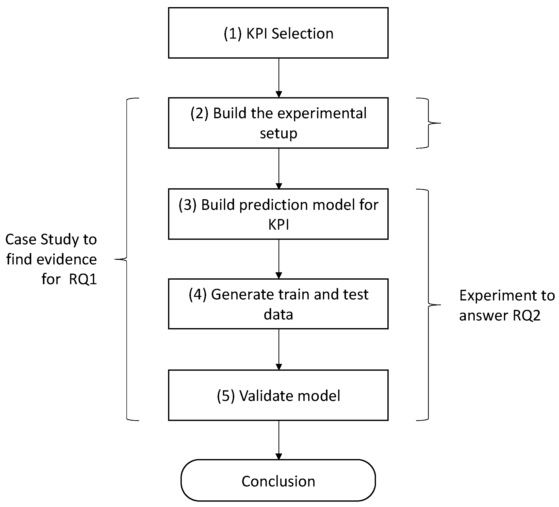
An experimental approach has been designed to address the “how” nature of RQ1 and to understand current technologies’ ease of use and limitations, thus answering both RQ1 and RQ2. The experiment was elaborated following the steps in Figure 1. Going through the process of setting up and executing the experiment also provided a comprehensive case study to give some evidence to answer RQ1, with the limitation that the chosen case study and technology will bias any conclusion drawn from a single case and cannot be generalized.

KPI selection (1) concerning the overall research question and RQ2 results in power consumption and duration. A more detailed consideration of the KPIs chosen in the case study is discussed in Section 3.4. The experimental setup (2) of a DT of a manufacturing site was built in several iterations following the maturity levels suggested in [28]: (i) the Digital Model, that is, the real object is connected to a computer model, and data are moved manually; (ii) the Digital Shadow, that is, data are moved automatically from the real object to the model while the responses are handled manually; and (iii) the Digital Twin, that is, full automation is achieved, where data flow automatically in both directions between the real and virtual objects. For the case study presented in this article, level (iii) of a DT is limited to feedback on the KPI to the machine operator as a means of decision support. Since changing the sequence of the manufacturing plan can only be performed manually, no further integration is possible. This is a limitation given by the infrastructure presented in Section 3.

The design and execution of the experiment (3,4,5,6) were elaborated in line with the method suggested by [29], which helps to avoid over-fitting of predictive models. Splitting of training and test data was performed randomly (50:50) and resampled and cross-validated with “Monte Carlo cross-validation” [29]. Section 3.5 explains the details of the experiment’s design in the case study context.

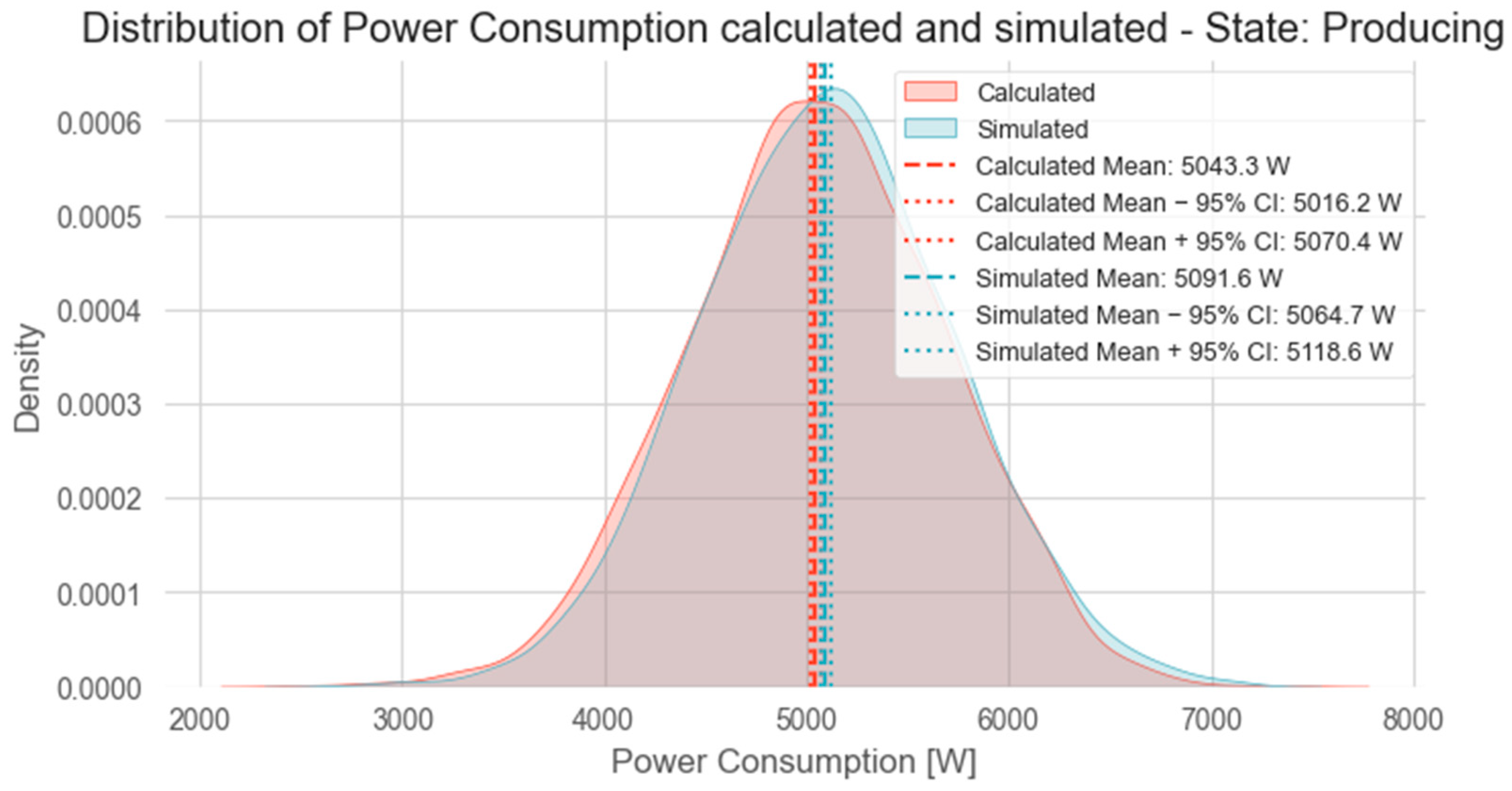
To ensure the robustness and accuracy of the model, a validation strategy inspired by established methodologies in computational model validation [29,30] is employed. This strategy involves comparing the simulation results with measured data, focusing on several key statistical metrics. First, the central tendency and variability of the model are assessed by comparing the means and standard deviations of the simulated and actual data. The mean provides insight into the model’s accuracy in predicting average behavior, while the standard deviation indicates the variability and consistency of the model’s predictions [30]. Further, the concept of confidence intervals, particularly the 95% confidence interval, is employed to understand better the statistical significance of the differences observed between the simulated and actual data. The confidence interval offers a range within which the true mean is expected to lie, which measures the reliability of the model’s predictions [30].

Independent two-sample t-tests were conducted to statistically ascertain the significance of the differences between the model’s predictions and actual measurements. This method tests the null hypothesis that there is no significant difference between the means of the two data sets. A p-value below the threshold of 0.05 indicates a statistically significant difference, suggesting that the model may need further calibration or adjustment [29]. This comprehensive validation approach not only ensures the accuracy and reliability of the model but also aids in identifying any potential overfitting issues or areas where model tuning might be necessary [29]. Rigorously comparing the model outputs with actual data using these statistical methods aims to enhance the model’s credibility and applicability in real-world scenarios.

3. Case Study Description

3.1. Description of the Floor-Ball Manufacturing Line

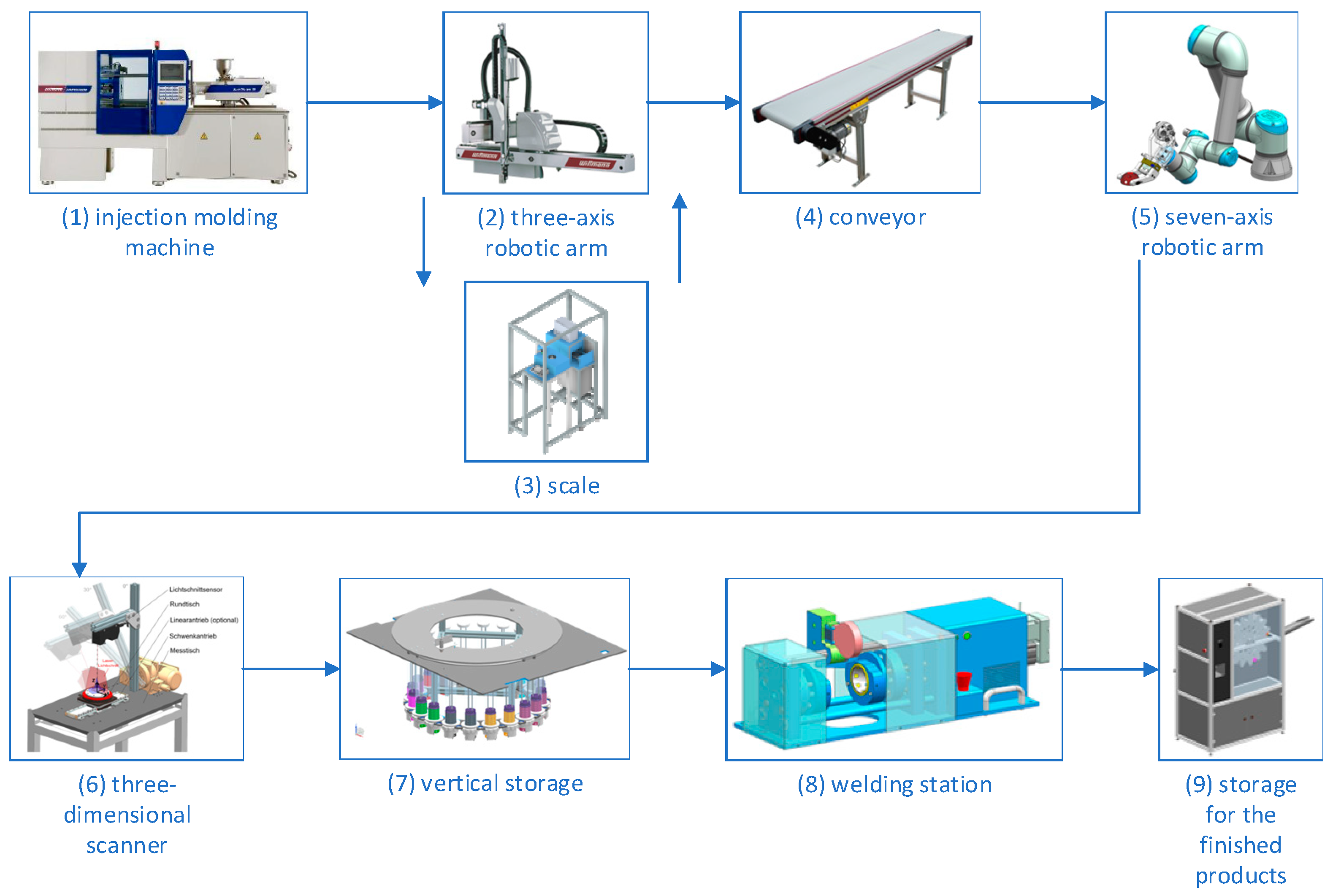
The smart factory built at the OST Rapperswil-Jona site consists of a production line for floor-ball. The production line comprises nine main elements, as shown in Figure 2. Following the same numbering as in Figure 1, the leading equipment is (1) a Battenfeld SmartPower 60, an injection molding machine to produce the ball halves. The second step of the manufacturing process (2) is a Wittmann W 818 T three-axis linear handling device, followed by (3) a Mettler Toledo scale to measure the weight of the ball halves. Then, a conveyor belt (4) transports the ball halves to the storage handling. The storage function is achieved through (5) a Universal Robots UR5e, which is a collaborative seven-axis robotic arm for the storage handling, (6) a custom-made three-dimensional scanner for the measurement of the shape precision, and (7) a custom-made vertical storage, consisting of plexiglass cylinders placed vertically following a circular arrangement around the seven-axis robot. In (8) a custom-made welding station, the halves are joined to manufacture a complete ball, which is finally stored in a (9) custom-made storage for the finished products with an interface for the withdrawal. The production line also includes a user interface of significant importance within the production process. Moreover, besides the leading equipment, many integrated components optimize the line’s usability and smartness. For example, a laser marker, sensors, control modules, switches, and connectors.

Regarding the monitoring and control architecture of the production line, various sensors are standard in the used equipment. Nevertheless, additional sensors have also been installed to monitor and evaluate the production process more precisely. In particular, Shelly 3EMs energy meters were installed on the injection molding machine so that the current power and total energy consumption could be measured and registered with an accuracy of 1%.

The whole process starts with melting plastic chipboard with the aid of the molding machine. Chips are manually placed inside a container. Once the machine has reached the proper temperature of pressure fusion, it is possible to produce the hockey ball halves. The production color is decided according to the needs dictated by the warehouse: if a particular color is lacking, its production proceeds. Once the molding process is over, the molding machine separates the two parts of the mold, from where it is possible to extract the manufactured product. The extraction takes place using a three-axis robotic arm (X-Y-Z) equipped with a robotic handle that, thanks to rotation, allows the extraction of the component from the previous machine. Once the half-balls have been extracted, they are placed on the conveyor belt from which two different storing configurations can be obtained:

• Operator storage. The half-balls fall directly from the conveyor into a box at the end of it. The products are then collected in a warehouse outside the line. This operation can be conducted to have more half-balls available than the number that can be contained in the vertical storage located above the seven-axis robot (limited).
• Robot storage. The conveyor belt stops half-balls at a specific location at the end of it. From here, the seven-axis robot can pick them up directly.

In the case of robotized storing, after the pick-up, the robot places the half-balls in an intermediate station that consists of a 3D scanner. This operation could also be carried out manually by an external operator. The purpose of the scan is to have information regarding the surface of the finished product and to collect data related to a specific production batch. Once the scanning is complete, the robot places the balls in the vertical storage, sorting them according to color. The information for the correct storing of the parts comes directly from the molding machine: when a specific color is produced, this information is entered into the shared database. Automatically, the robot will know in which store it must place the half-balls. Once the batch storing is finished, the robot waits to receive an order from the user interface. It is possible to configure a customer-specific floor-ball through a user interface. By selecting the various colors and clicking on the order button, the customer will receive a ticket with a QR code corresponding to the order placed. Thus, the assembly phase begins: the robot removes the selected color half-balls from the vertical store and places them in an assembly station.

Here, the half-balls are held by a locking system with the inner sides facing each other. The assembly is carried out by a plate of conductive material that intervenes between the two halves once heated. The half-balls are placed close to the plate and kept in this position for enough time to melt the plastic surface. Then, the halves are separated, and the plate is removed. The machine can now complete the finished product, which consists of the union of the two halves. Once the assembly phase is complete, the ball falls into a slide placed in a circular store, equating it to a circular carousel. The product will remain in the store until the user redeems the order. The redemption is accomplished by presenting the ticket obtained from the order to a QR code reader. At this point, it will be possible to collect the product ordered.

3.2. DT Information Model Description

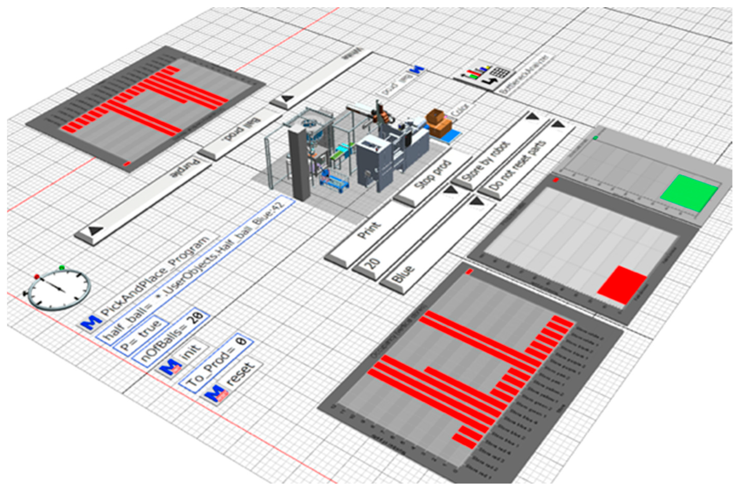
Siemens Tecnomatix Plant Simulation (TPS) [31] has been used to model and display the floor-ball manufacturing line. TPS is an object-oriented 3D software (version 2201) that allows modeling and simulates discrete events and provides advanced analytical tools to optimize material flow, resource utilization, and logistics at different planning levels. Its modeling platform can represent a production plant in 2D or 3D, providing preset elements for good simulations. It also allows importing external graphic models to analyze space management, safety, efficiency, and worker comfort.

The use of external resources predominantly facilitated the development of the 3D model within Siemens TPS. Specifically, this process did not involve the application of existing TPS libraries. Instead, the model’s structure was assembled primarily from 3D models supplied by the machine manufacturers. These models offered a realistic depiction of the machinery integral to our floor-ball manufacturing line. Additionally, bespoke designs created in the development of the Smart Factory were incorporated. Importing these external models into the TPS platform created a faithful and functional representation of the manufacturing process, allowing for a comprehensive analysis of various operational parameters.

3.3. DT Data Processing Module and Communication Mechanism

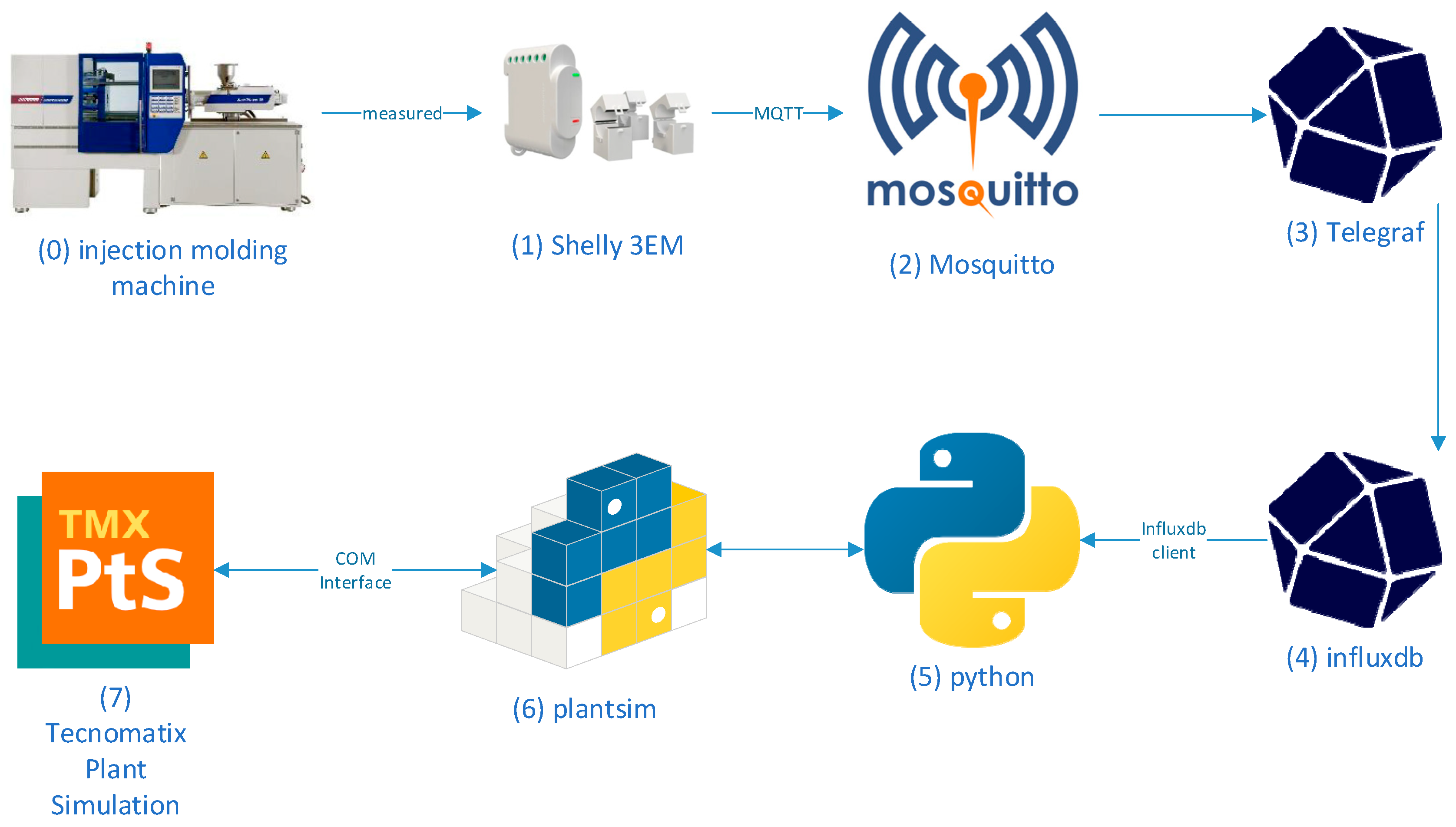
Implementing a data processing module and communication mechanism enhances a DT system. The coupling of the DT with physical resources is typically accomplished through a toolchain that enables data collection, processing, and storage as close to real-time as possible. This section describes the specific toolchain used in the research activities described in this study. Coupling of the DT with physical asset has been achieved through the toolchain, as shown in Figure 3: (1) Shelly 3EM energy sensors were integrated into the main power inlet of the (0) injection molding machine and connected over MQTT to a broker, here (2) Mosquitto (version 2.0.15), running on a Linux-based server. From Mosquitto, data were routed through (3) Telegraf (version 1.24.2), an agent to collect, process, and write data, and (4) InfluxDB (version 2.4.0), a time-series database. Then, these stored data could be queried from a (5) Python script. The bidirectional connection between Python and the (7) TPS simulation was established with the package (6) Plantsim Python [32]. The Python script generates a linear model using the training dataset (refer to Section 3.5 for additional details on data splitting). This model is then utilized to configure parameters within TPS via Plantsim. The utilization of a linear model implies the usage of past data, while it can be used with current data to enable data processing close to real-time (limited by the processing speed). In addition, the model can improve when more past data are available.

The Plantsim Python package serves as an effective medium for communicating with the TPS software. This package is executed over the COM interface and includes mappings for complex PlantSim data types, such as tables, facilitating smoother interaction with the software. However, it is essential to note that Tecnomatix, Plant Simulation, and related terms are the brand names of Siemens, while this package is not an official product of Siemens.

The functionalities provided by the Plantsim Python package encompass, but are not limited to:

• Launching the TPS software by invoking it with the version (optional) and license type information.
• Loading a specified model by providing the respective file path and name.
• Accessing and modifying all simulation parameters via their designated path and name.
• Reading and updating tables by referring to them through their particular path and name.
• Manipulating the simulation controls such as start, stop, and reset.
• Implementing advanced SimTalk commands, although this feature was not utilized in this study.
• Terminating both the model and the software.

These operations transpire between the Plantsim Python package, as represented in Figure 3 (Item 6), and the Siemens TPS software, denoted in Figure 3 (Item 7). The 3EM by Shelly is a simple-to-use and easily integrable energy meter with good availability, selected primarily for its ability to measure three-phase current, wireless connectivity, and compatibility with MQTT.

3.4. KPIs Definition and Assessment

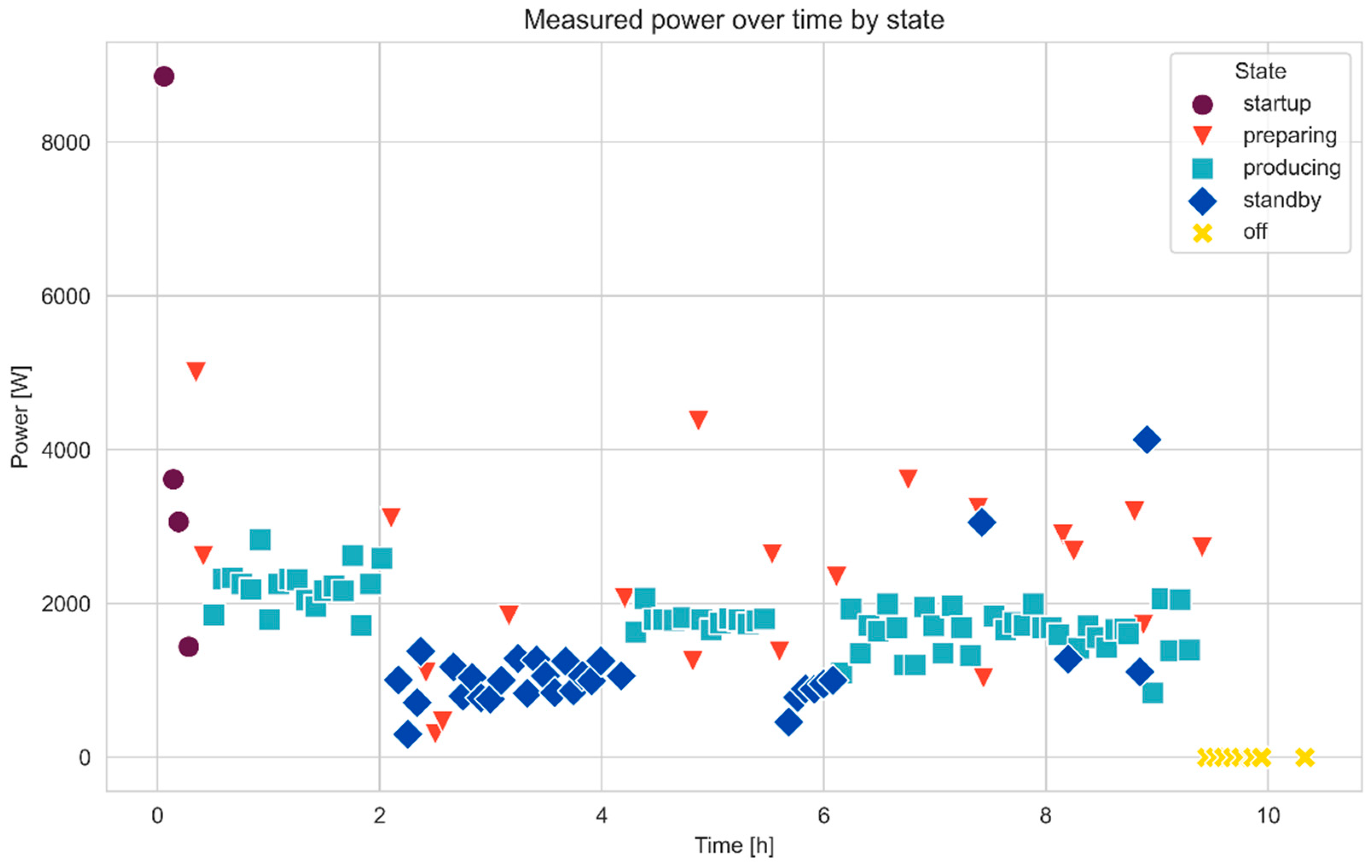
Key Performance Indicators (KPIs) have been identified to evaluate DT performance quantitatively. Electricity consumption and the duration of consumption, which are crucial factors in the manufacturing sector, have been specifically highlighted. These metrics are recorded for each production stage, including off, preparing, producing, and standby.

The collected dataset is divided into training and testing sets to validate the simulation model (see Section 3.5). The electricity consumption from the training set, measured in Watts for each production stage, is combined with the corresponding duration of consumption. These combined metrics of power and energy consumption serve as the input parameters for the DT.

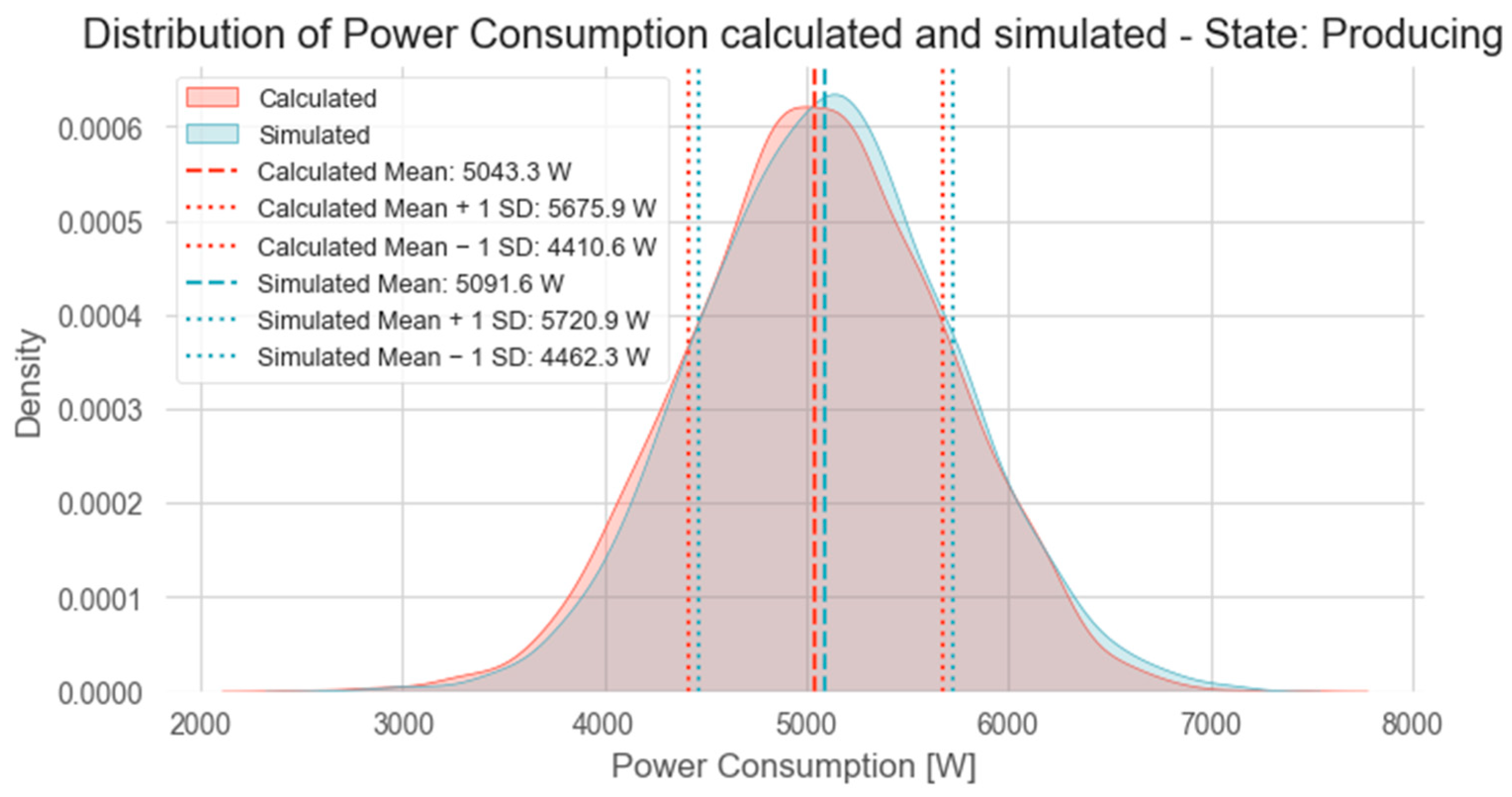
The electricity consumption predicted by the DT is compared with actual data from the testing set. The accuracy of the DT prediction is quantified according to the metrics described in Section 2. As a single event may lead to high deviation due to an uneven split, the simulation is repeated multiple times to provide a statistically grounded depiction of the deviation. These quantitative evaluations aim to thoroughly and accurately assess DT performance.

3.5. Design of the Experiment

The experiment centered around the Battenfeld injection molding machine with a primary objective of measuring the KPIs outlined in Section 3.4. After data capture, data were labeled according to observations made during production to identify the different states (off, standby, preparing, and producing). Considering the significant variance in the time steps during which data from the Shelly 3EM were recorded and the uncertainty about the events between these steps, power consumption was computed from the change in total energy consumption, measured in Wh. This total was then divided by the desired time steps to yield power consumption in Watts (W), making the result independent of the time steps.

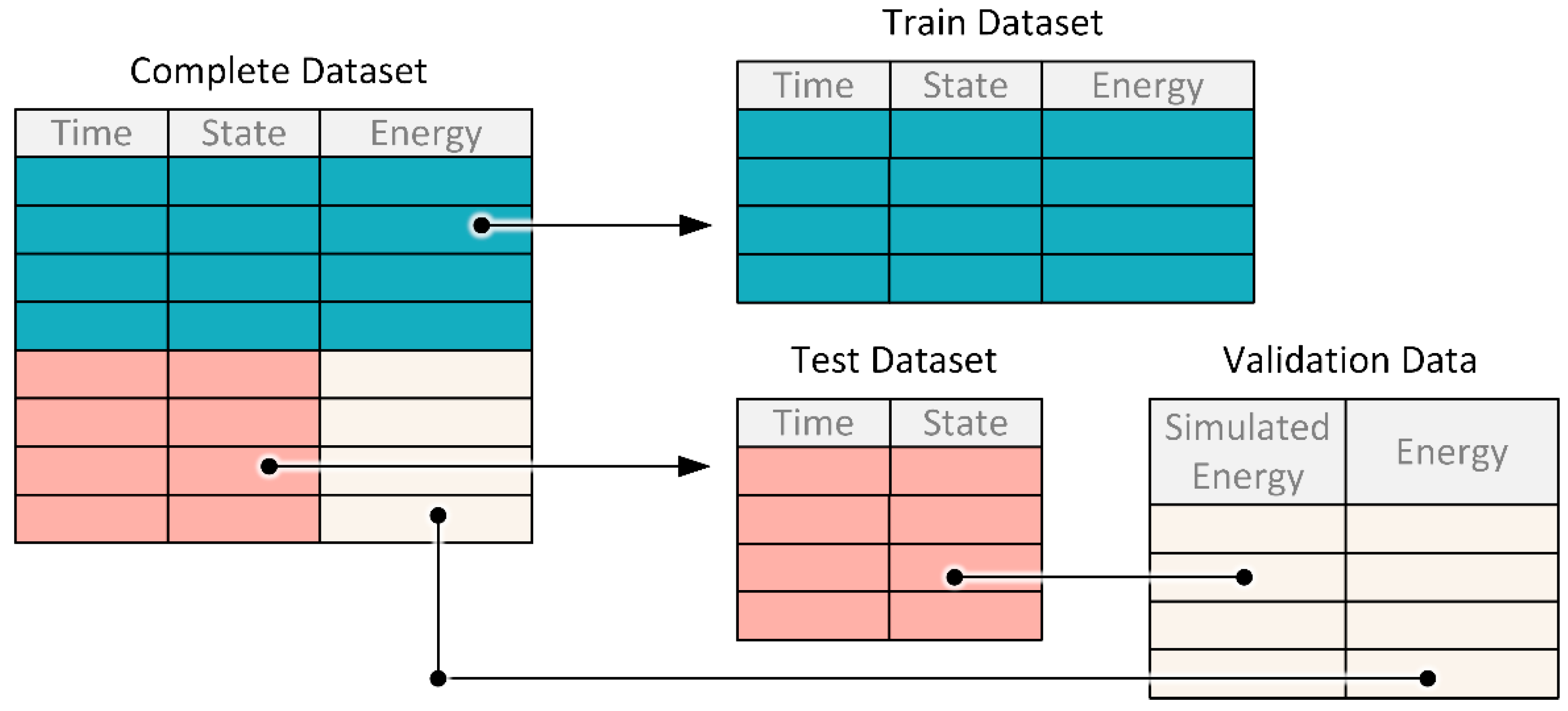
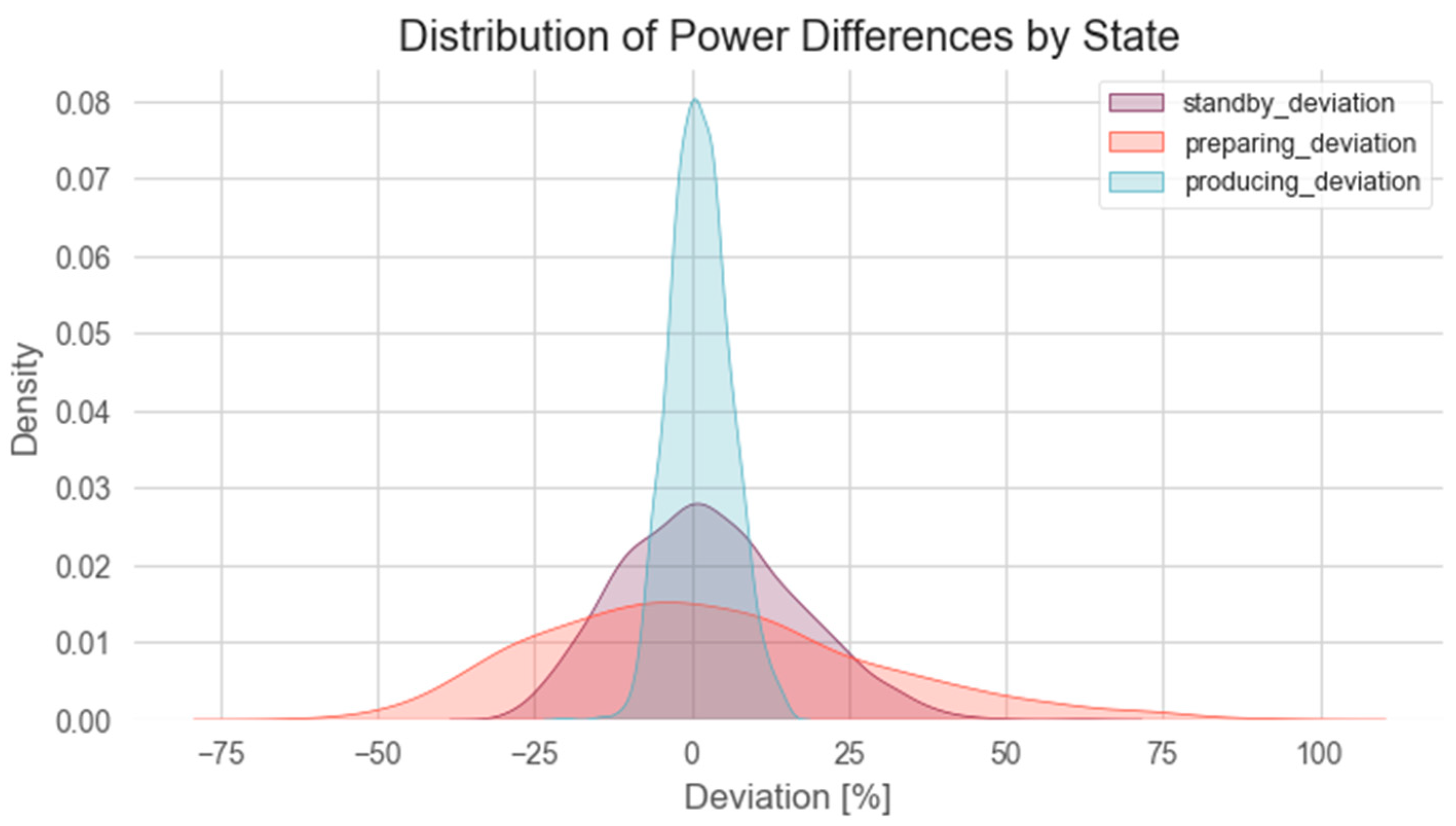
With these steps completed, the dataset was divided into two sets (see Figure 4): one for training and the other for testing the digital model, and over 2000 simulations were conducted using random test–train splits with a ratio of 50:50. Input data for each simulation consisted of power consumption [W] for each production state from the train set, associated with the duration [h] of each operating state from the test set. The simulation output is the energy consumption [Wh] for each state. The test power consumption [W] of the operating states was calculated with the test set, and the expected energy consumption [Wh] was derived by multiplying the test power consumption [W] by the corresponding duration [h] for each state’s test data. The simulation result and test data were then compared using the percentage deviation of the simulation from the calculated value from measurements.

4. Results

4.1. Design and Development of Floor-Ball Manufacturing DT

The virtual copy of the floor-ball manufacturing line appears in Figure 5. The resulting model closely follows the physical model present in real-world laboratories. From a simulation point of view, the DT allows all possible production scenarios to be analyzed, guaranteeing easy availability of production data (machine times, store occupancy, machine use). The model enables the production of half-balls to be simulated and the ordering of the finished product through a user interface representing the configurator. The simulation allows analysis of the system’s behavior in a whole operating situation by implementing a random order generator. In the described configuration, the simulation output allows us to obtain information on potential improvements to be applied in the line. It also evaluates the replacement or a different machinery configuration to meet customer demand. Parameters for the simulation are captured from the interfaces offered by the different assets. For some time and velocity values (e.g., speed of conveyor, time to scan a ball-half), no digital interface was available; thus, these values were captured by hand. KPIs from the simulation are visualized inside the DT.

4.2. Connection between Real Machines and Their DT

The connection between the DT and the physical assets was achieved for the injection molding machine, as it has the highest impact on power consumption. The toolchain was implemented as described in Figure 3. One significant insight gives the critical role of timestamps, which should be recorded as close to the machine as possible to ensure the utmost precision in data collection. The delay is particularly significant if the processing times in the toolchain are high.

Figure 6 illustrates the power consumption in various states over a time window of approximately 10 h. During this time, different products were produced, resulting in varying levels of power required for preparation and production.

4.3. Using the DT to Predict Energy Consumption Based on a Production Cycle

Following the design of experiments described in Section 3.5, captured data were split into training and test datasets. It is important to note that in the subsequent visualizations, the power consumption value for the “off” state was omitted, as it consistently equals zero across all cases. This omission simplifies visual data representation without losing critical information. Figure 7 shows the percentage deviation between the mean power consumption of the test dataset and the simulation result from each simulation.

The validation process of a DT, mainly when the process is widely distributed, needs an extensive number of simulations to encapsulate the broad range of possible results. A striking pattern emerged during the initial five hundred simulations, presenting a skewed distribution. Upon deeper analysis and with the help of additional simulations, the nature of this anomaly became clearer. It was discerned that an extra computational load, in addition to the simulation on the simulation device, could impact the communication between Python and the TPS COM interfaces by delaying packages. This interference occurs due to the delay in commands, thereby influencing the simulation results. The experiment was repeated with 1500 simulations conducted without parallel loads to circumvent the issue.

The mean and standard deviation were compared for each state to assess the central tendency and variability. Figure 8 compares the simulation result and the expected power consumption for the state “producing” to assess the model’s accuracy. The expected power consumption was derived from input data in each simulation, namely, the test dataset.

Table 1. Comparison of the distribution’s characteristics of the states Standby, Preparing, and Producing.

	Standby	Preparing	Producing
Train dataset mean	1266.8 W	1402.8 W	5043.3 W
Train dataset standard deviation (STD)	246.7 W	362.2 W	632.6 W
Train dataset percentage STD of mean	19.5%	25.8%	12.5%
Simulated Mean	1295.0 W	1400.9 W	5091.6 W
Simulated standard deviation (STD)	277.9 W	390.9 W	629.3 W
Simulated percentage STD of mean	21.5%	27.9%	12.4%

lists the key figures for the comparison visualized in Figure 8 for each state of the machine.

To attain a deeper understanding of the statistical significance of the result, the 95% confidence interval (CI) is calculated for each process. Figure 9 shows the density graph of the training dataset’s calculated mean and the simulation’s output with the mean and the corresponding 95% confidence intervals on each side.

Table 2. Comparison of the confidence intervals of the states Standby, Preparing, and Producing.

	Standby	Preparing	Producing
Train dataset mean	1266.8 W	1402.8 W	5043.3 W
Train dataset mean − 95% CI	1256.3 W	1387.3 W	5016.2 W
Train dataset mean + 95% CI	1277.4 W	1418.3 W	5070.4 W
Simulated Mean	1295.0 W	1400.9 W	5091.6 W
Simulated mean − 95% CI	1283.1 W	1384.2 W	5064.7 W
Simulated mean + 95% CI	1306.9 W	1417.7 W	5118.6 W
Overlapping	No	Yes	Yes

compares the confidence intervals of the different states (Standby, Preparing, and Producing) of the molding process. In contrast to the standby state, overlapping the confidence intervals at the preparing and producing state does not allow rejection of the null hypothesis (which states that the true means are the same) right away.

To check whether the null hypothesis can be rejected statistically, a two-sided t-test is calculated (see

Table 3. Comparison of the T-Test results of the states Standby, Preparing, and Producing.

	Standby	Preparing	Producing
T-statistic	−3.473	0.159	−2.479
p-value	0.001	0.875	0.013
Result	Statistically significant difference between calculated and simulated data	No statistically significant difference between calculated and simulated data	Statistically significant difference between calculated and simulated data

), which allows the rejection of the null hypothesis when the p-value is below 0.05. The t-test shows that only the true mean of the preparing state can be the same. At the standby and producing state, the true mean differs statistically significantly.

5. Discussion

The results presented show a DT—or, at its current state, rather a digital shadow—of a production line on two levels.

• Macro-level: Digital representation of the assembly line, capable of simulating the production of different product configurations.
• Micro-level: A detailed trained model of the power consumption of one particular machine.

5.1. Implementation of Toolchain and Macro-Level DT

The development of the macro-level model was relatively straightforward, based on existing technology. The main barrier faced was interoperability between the involved components. The attempt to establish end-to-end communication on a commercial out-of-the-box approach was abandoned due to project time limitations and complexity. Changing to in-house development of interfaces turned out to be faster in implementation and better in performance. Nevertheless, the same approach may not be an option for companies willing to implement a DT, particularly SMEs. This is expected to be the main barrier to DT implementation at the industrial level. Referring to the research question RQ1, a trade-off can be observed between commercial tools that focus on a wide range of use cases versus individually programmed software that serves one particular use case. The commercial tools seen in the case study proved to be robust. Still, due to their generic data models, they compromise transmission time and quickly result in high complexity and slow implementation time. On the other hand, custom-built tools can optimize for specific use cases but might have scalability and long-term operation limitations. In the case study setup, the mix of both commercial and individual software seems a reasonable approach that allows relaying on a robust IoT Stack on the one hand but optimizes time issues and uses case-specific data treatment such as tagging or cleansing with individual software. This observation’s main limitation is that it refers to one case study. For future work, multiple case studies have to be analyzed to extract implementation patterns of industrial DTs. An approach similar to [33] could be considered but with a dedicated focus on DT implementation.

5.2. Implementation Prediction Model at Microlevel

At the micro-level, which relates to RQ1, Figure 6 shows disparate deviations for the different steps in a manufacturing cycle. While the power consumption of “production” can be simulated with promising accuracy, the deviation of the “preparing” state is very high. This can be partially explained by the usage of different electric motors in the respective steps, as well as the heating of the plastic chips for the injection phase. This observation leads to an interesting conclusion. For some steps, data can be measured, trained once, and reused during the DT lifecycle without further physical sensors. For other steps, a persistent connection is needed to update the model continuously based on process and product complexity.

Section 4 analysis suggests that discrete event simulation possesses significant potential to act as a DT model for simulating and predicting power consumption in a factory setting. This conclusion is drawn from the validation process that involved a detailed comparison of simulated results with actual measured data across various operational states of the factory’s machinery. The validation approach primarily focused on comparing central tendency and variability metrics, namely the mean and standard deviation, between the training dataset (actual measurements) and the simulation results. The comparisons were made for the Standby, Preparing, and Producing states, as detailed in Table 1. This first approach showed that the means are close to each other with a comparable standard deviation. This allows us to deduct that the simulations have a similar data spread compared with actual data and, therefore, can mimic the real situation roughly. Further, the observed statistical significance was reinforced by calculating 95% confidence intervals. While the CI of the Standby state does not, the CI of the Preparing and Producing states overlap, suggesting immediate grounds to reject the null hypothesis in the Standby state but not in the Preparing and Producing states. A two-sided t-test was conducted for each state to validate these observations further. The results revealed in the Standby and Producing states, the p-values were 0.001 and 0.013, respectively, indicating statistically significant differences between the calculated and simulated data. However, with a p-value of 0.875 for the Preparing state, no statistically significant difference was observed, suggesting that the simulated mean could be the same as the actual mean in this state.

In conclusion, the findings underscore the viability of discrete event simulation as a DT model in a factory setting for power consumption prediction. While the simulation showed high fidelity in certain states (such as Preparing), some discrepancies in others (such as Standby and Producing) highlight the need for ongoing model tuning and refinement. This study demonstrates that discrete event simulations can effectively mirror real-world scenarios with careful calibration and validation, making them valuable for predictive analysis in industrial applications. Discrete event simulations may not effectively capture continuous system dynamics, potentially missing key changes in industrial processes. Often relying on linear models, these simulations can oversimplify complex, nonlinear interactions found in industrial setups, affecting their representational accuracy. Additionally, scalability becomes a challenge as system complexity increases, and the time-intensive nature of these simulations hinders their use in real-time decision-making. Moreover, the accuracy of these simulations heavily depends on the quality of input data. Inaccuracies in data can lead to significant deviations from actual scenarios, emphasizing the need for precise data collection.

5.3. Combination of Macro and Micro Level

By collecting and predicting power consumption data of all assets and entering it into the simulation model, different scenarios can be analyzed to find an optimal solution that satisfies lead-time expectations, costs, and the ecological footprint through lower energy consumption. Thus, optimization of power consumption requires linking the macro and micro models of all relevant components in the process. However, the complexity of such a model can be simplified by a thorough analysis of the deviation of single assets based on process and product complexity, as illustrated in Figure 6.

Applying such an optimization on a production line, as presented in this study, might also affect the quality. For example, the timing and parameters of the molding machine are directly correlated to the quality of the finished product. Therefore, this station’s optimization should be followed by a quality test on the half-balls to verify that their characteristics meet the required standards. The interface to the quality measurement system is already available in the testing facility and must be integrated into the DT to validate simulation against product quality.

6. Conclusions

Digital twin technology is one of the key technologies to achieve the fusion of virtual and physical models aiming to increase industrial process efficiency and effectiveness and reduce the ecological footprint. This study aims to answer the research question: “How can the implementation of digital twin technology help to optimize the balance between power consumption and productivity, taking into account existing barriers and limitations?” This study describes a practical case study implemented at the Smart Factory of OST to answer the research question. The digital representation of the floor-ball production line investigated has two levels of detail: the macro level rebuilds the assembly line and can simulate the production of different product configurations. In contrast, the micro level is a specific molding machine model optimized through a training process for power consumption assessment. The results show a good convergence between measured and simulated data, suggesting that digital twins can be a promising technology to address the energy efficiency topic in the manufacturing processes. Nevertheless, the experimental test also underlined several practical limitations to digital twin applications. A trade-off between commercial tools and tailored programmed software has been identified. Moreover, discrete event simulations showed some discrepancies in some of the investigated processes (i.e., Standby and Producing), thus indicating the need for ongoing model tuning and refinement.

The next step of DT development at the Smart Factory of OST will focus on optimizing the manufacturing process to reduce the ecological footprint while guaranteeing the requested quality standard. The assessment procedure will include collecting several data in addition to energy consumption (such as injection temperature, heating and molding times, and other variables considered influential through SMS) and the definition of an equation for energy consumption to efficiently perform an F-Test with the already developed software, evaluating the influence of variables on total energy consumption.

References

1. Alcacer, V.; Cruz-Machado, V. Scanning the Industry 4.0: A literature review on technologies for manufacturing systems. Eng. Sci. Technol. Int. J. 2019, 22, 899–919. [Google Scholar] [CrossRef]
2. Usman, S.; Mehmood, R.; Katib, I.; Albeshri, A. Data Locality in High Performance Computing, Big Data, and Converged Systems: An Analysis of the Cutting Edge and a Future System Architecture. Electronics 2023, 12, 53. [Google Scholar] [CrossRef]
3. Lu, Y.; Liu, C.; Kevin, I.; Wang, K.; Huang, H.; Xu, X. Digital twin-driven smart manufacturing: Connotation, reference model, applications and research issues. Robot. Cim.-Int. Manuf. 2020, 61, 101837. [Google Scholar] [CrossRef]
4. Leng, J.; Wang, D.; Shen, W.; Li, X.; Liu, Q.; Chen, X. Digital twins-based smart manufacturing system design in Industry 4.0: A review. J. Manuf. Syst. 2021, 60, 119–137. [Google Scholar] [CrossRef]
5. Tuegel, E.J.; Ingraffea, A.R.; Eason, T.G.; Spottswood, S.M. Reengineering aircraft structural life prediction using a digital twin. Int. J. Aerosp. Eng. 2011, 2011, 154798. [Google Scholar] [CrossRef]
6. ISO 23247-1:2021; Automation Systems and Integration—Digital Twin Framework for Manufacturing—Part 1: Overview and General Principles. International Organization for Standardization: Geneva, Switzerland, 2021.
7. ISO 23247-2:2021; Automation Systems and Integration—Digital Twin Framework for Manufacturing—Part 2: Reference Architecture. International Organization for Standardization: Geneva, Switzerland, 2021.
8. Muanis Persechini, M.A.; Goncalves Jota, F. Centralized and distributed control architectures under Foundation Fieldbus network. ISA Trans. 2013, 52, 149–161. [Google Scholar] [CrossRef] [PubMed]
9. Obite, F.; Tumunoiyowuna Jaja, E.; Ijeomah, G.; Jahun, K.I. The evolution of Ethernet Passive Optical Network (EPON) and future trends. Optik 2018, 167, 103–120. [Google Scholar] [CrossRef]
10. Beshley, M.; Hordiichuk-Bublivska, O.; Beshley, H.; Ivanochko, I. Data Optimization for Industrial IoT-Based Recommendation Systems. Electronics 2023, 12, 33. [Google Scholar] [CrossRef]
11. GE Website. Available online: https://www.ge.com/digital/iiot-platform (accessed on 25 January 2023).
12. Siemens Website. Available online: https://www.plm.automation.siemens.com/global/it/our-story/glossary/digital-twin/24465 (accessed on 25 January 2023).
13. ABB Website. Available online: https://global.abb/topic/ability/en (accessed on 25 January 2023).
14. Microsoft Website. Available online: https://azure.microsoft.com/it-it/products/digital-twins/ (accessed on 25 January 2023).
15. Wang, J.; Li, X.; Wang, P.; Liu, Q. Bibliometric analysis of digital twin literature: A review of influencing factors and conceptual structure. Tecnol. Anal. Strateg. 2022, 2022, 1–15. [Google Scholar] [CrossRef]
16. Cimino, C.; Negri, E.; Fumagalli, L. Review of digital twin applications in manufacturing. Comput. Ind. 2019, 113, 103130. [Google Scholar] [CrossRef]
17. Onaji, I.; Tiwari, D.; Soulatiantork, P.; Song, B.; Tiwari, A. Digital twin in manufacturing: Conceptual framework and case studies. Int. J. Comput. Integr. Manuf. 2022, 35, 831–858. [Google Scholar] [CrossRef]
18. Guo, D.; Li, Q.; Liu, P.; Shi, X.; Yu, J. Power shortage and firm performance: Evidence from a Chinese city power shortage index. Energ. Econ. 2023, 119, 106593. [Google Scholar] [CrossRef]
19. Xiao, Z.; Gao, J.; Wang, Z.; Yin, Z.; Xiang, L. Power shortage and firm productivity: Evidence from the World Bank Enterprise Survey. Energy 2022, 247, 123479. [Google Scholar] [CrossRef]
20. Taisch, M.; Stahl, B.; Vaccari, F.; Cataldo, A. A Production-State Based Approach for Energy Flow Simulation in Manufacturing Systems. In Advances in Production Management Systems. Sustainable Production and Service Supply Chains. APMS 2013. IFIP Advances in Information and Communication Technology, 1st ed.; Prabhu, V., Taisch, M., Kiritsis, D., Eds.; Springer: Berlin/Heidelberg, Germany, 2013; pp. 227–234. [Google Scholar]
21. Mousavi, S.; Thiede, S.; Li, W.; Kara, S.; Herrmann, C. An integrated approach for improving energy efficiency of manufacturing process chains. Int. J. Sustain. Eng. 2016, 9, 11–24. [Google Scholar] [CrossRef]
22. Karanjkar, N.; Joglekar, A.; Mohanty, S.; Prabhu, V.; Raghunath, D.; Sundaresan, R. Digital twin for energy optimization in an SMT-PCB assembly line. In Proceedings of the 2018 IEEE International Conference on Internet of Things and Intelligence System IOTAIS, Bali, Indonesia, 1–3 November 2018; pp. 85–89. [Google Scholar]
23. Cabrucci, A.; Accorsi, R.; Bortolini, M.; Guzzini, A.; Nyffenegger, F.; Pellegrini, M.; Saccani, C. Design and development of a Digital Twin for a production line: A case study from the winter-sport sector. In Proceedings of the 27th Summer School Francesco Turco, Sanremo, Italy, 7–9 September 2022. [Google Scholar]
24. Ugarte, M.; Etxeberria, L.; Unamuno, G.; Bellanco, J.L.; Ugalde, E. Implementation of Digital Twin-based Virtual Commissioning in Machine Tool Manufacturing. Procedia Comput. Sci. 2022, 200, 527–536. [Google Scholar] [CrossRef]
25. Zhong, D.; Xia, Z.; Zhu, Y.; Duan, J. Overview of predictive maintenance based on digital twin technology. Heliyon 2023, 9, e14534. [Google Scholar] [CrossRef] [PubMed]
26. Beruvides, G.; Quiza, R.; del Toro, R.; Castaño, F.; Haber, R.E. Correlation of the holes quality with the force signals in a microdrilling process of a sintered tungsten-copper alloy. Int. J. Precis. Eng. Man. 2014, 15, 1801–1808. [Google Scholar] [CrossRef]
27. Castaño, F.; Haber, R.E.; del Toro, R.M. Characterization of tool-workpiece contact during the micromachining of conductive materials. Int. J. Precis. Eng. Man. 2017, 83, 489–505. [Google Scholar] [CrossRef]
28. Kritzinger, W.; Karner, M.; Traar, G.; Henjes, J.; Sihn, W. Digital Twin in manufacturing: A categorical literature review and classification. IFAC Pap. 2018, 51, 1016–1022. [Google Scholar] [CrossRef]
29. Kuhn, M.; Johnson, K. Over-Fitting and Model Tuning. In Applied Predictive Modeling, 1st ed.; Kuhn, M., Johnson, K., Eds.; Springer: New York, NY, USA, 2013; pp. 61–92. [Google Scholar]
30. Oberkampf, W.L.; Barone, M.F. Measures of agreement between computation and experiment: Validation metrics. J. Comput. Phys. 2006, 217, 5–36. [Google Scholar] [CrossRef]
31. Siemens Website. Available online: https://plm.sw.siemens.com/en-US/tecnomatix/products/plant-simulation-software/ (accessed on 25 January 2023).
32. Python Package Index Repository. Available online: https://pypi.org/project/plantsim/ (accessed on 30 August 2023).
33. Helbling, S.; Nyffenegger, F. Planning the technical implementation of smart services based on their business model. In Proceedings of the IFIP 20th International Conference on Product Lifecycle Management, Montreal, QC, Canada, 9–12 July 2023. [Google Scholar]
Figure 1. Visualization of the experimental approach.
Electronics 12 04979 g001
Figure 2. PFD of the main components in the smart factory production line.
Electronics 12 04979 g002
Figure 3. The schematization of the toolchain applied in the case study.
Electronics 12 04979 g003
Figure 4. Visualization of the test–train split and data used for running the DT with sample data from measured data.
Electronics 12 04979 g004
Figure 5. Result of floor-ball manufacturing line modeling in TPS.
Electronics 12 04979 g005
Figure 6. Power consumption of each divided section in different states of the injection molding machine.
Electronics 12 04979 g006
Figure 7. Density graph of the deviation between the simulation and test data.
Electronics 12 04979 g007
Figure 8. Density graph of the training dataset’s calculated mean and the simulation’s output with the mean and standard deviation.
Electronics 12 04979 g008
Figure 9. Density graph of the training dataset’s calculated mean and the simulation’s output with the mean and the corresponding 95% confidence intervals on each side.
Electronics 12 04979 g009