Few-Shot Classification Based on the Edge-Weight Single-Step Memory-Constraint Network

Abstract

Few-shot classification algorithms have gradually emerged in recent years, and many breakthroughs have been made in the research of migration networks, metric spaces, and data enhancement. However, the few-shot classification algorithm based on Graph Neural Network is still being explored. In this paper, an edge-weight single-step memory-constraint network is proposed based on mining hidden features and optimizing the attention mechanism. According to the hidden distribution characteristics of edge-weight data, a new graph structure is designed, where node features are fused and updated to realize feature enrichment and full utilization of limited sample data. In addition, based on the convolution block attention mechanism, different integration methods of channel attention and spatial attention are proposed to help the model extract more meaningful features from samples through feature attention. The ablation experiments and comparative analysis of each training mode are carried out on standard datasets. The experimental results obtained prove the rationality and innovation of the proposed method.

1. Introduction

Labeling data requires time and labor, but humans only need a small amount of learning to realize the cognition and analysis of new things. This small amount of learning is the gap between humans and machines. Therefore, employing the human learning method to achieve classification with a small amount of label samples is a problem that researchers need to solve [1,2,3,4,5]. A lack of label samples makes the training with few-shot classification different from other big-data networks and has produced many methods to solve the few-shot classification problem, including transfer learning [6,7], meta-learning [8,9], metric learning [10,11], data enhancement [12,13], etc. At present, in the field of image classification, the application of the Graph Neural Network (GNN) method in few-shot classification maximizes the use of the connections between samples and learns intra-class relationships and inter-class connections by building graph structures [14]. The aim is to build small classification tasks continuously and gradually realize “the big from the small” so that a model can continuously learn how to realize classification from a small number of samples and generalize a larger model at the same time [15]. Its unique topological structure has good interpretability and a more intuitive display. With the gradual rise of GNN, a few-shot classification algorithm based on GNN not only has long-term development and economic value but also has far-reaching research significance and research value in the military, medical, aesthetic, security, and other industries with missing label data [16].

With the application of the GNN algorithm in the research of few-shot classification, the accuracy of few-shot classification has gradually improved. The model based on the migration network cannot solve classification problems with differences in the spatial distribution of samples. Moreover, with the increase in the number of layers in deep networks, few-shot classification is prone to overfitting. When shallow networks are used, rich deep features cannot be extracted, so the use of many networks is very limited. Although the classification performance of many deep networks is good enough, in the field of few-shot classification, the problem is of too many parameters and too few samples. The GNN-based classification model has emerged in recent years, introducing graph structure, combining meta-learning training strategies, establishing associations between samples, updating each other through edge nodes, and using explicit edge annotation as a prior condition. Its classification performance is not inferior to that of migration networks and some deep networks. In summary, this paper will study the small-sample classification algorithm based on the GNN model, which has both development prospects and research value.

In this paper, according to the relationship between the edges and nodes of a graph structure, a new graph structure is constructed specifically for edge-weight features, and the implicit distribution of edge-weight data is added to update the edge node. In the network, we learn both instance-level features and distribution-level features to enrich the feature data and make use of the feature data from a more comprehensive perspective. In addition, from the perspective of improving the feature extraction effect, this paper uses the attention mechanism to learn the channel and spatial weights of the initial node-feature extraction module so that the network can pay attention to more meaningful channels and image spatial positions. At the same time, through this method, the model can improve the generalization ability of sample-category transformation in different tasks.

2. Related Work

In recent years, it has been common to train models using big data and achieve success both in the field of machine learning and deep learning. Many researchers often worry about their datasets rather than how to build models. In-depth methods from different aspects have different significance. The emergence of transfer learning has greatly promoted the development of small-sample learning so that classification can be realized after fine-tuning the model pre-trained under big data with only a small amount of marking data [17,18]. However, such methods require the source domain to be similar to the target domain and have a mappable space. When such conditions are not met, the classification results are not as expected. The sample data are too small, and the fine-tuned parameters still fail to achieve the requirements of classification. In addition, even if methods similar to data enhancement can increase the sample size, it still cannot fundamentally solve the problem of few-shot classification [19,20,21]. According to the evolution time of the method, the existing few-shot classification methods are divided into four categories: transfer learning, data enhancement, metric learning, and meta-learning [22].

In 2016, Ganin et al. presented the domain-adversarial training of neural networks at the TMLR academic conference [23]. Transfer learning fixes a large number of layer parameters by adopting a large data pre-training model similar to the target data and improving the situation where a small number of labeled data cannot train a good model using few-shot classification to fine-tune the parameters of a specific layer [24]. The generation of transfer learning prompts few-shot learning, but when the probability distribution or spatial distribution of samples between the training model data domain and the few-shot data domain is very different, the model is difficult to establish.

In the problem of few-shot classification, many studies start from data and increase the number of label samples, so we need to achieve data enhancement. Data enhancement is designed to generate more new data in line with the overall distribution of image samples on the basis of existing image samples through synthesis, style migration, geometric transformation, and other operations [25,26]. The main idea of semantic feature augmentation in few-shot learning published by Zitian Chen et al. in 2018 is data enhancement, mapping the visual feature information of a small number of image samples to semantic space through a certain method [27] so that each sample can acquire richer semantic features. The method expands the data in the semantic space by adding Gaussian noise to the sample and nearest-neighbor matching. Finally, the method maps the supplementary semantic information back to the visual space to expand the sample.

From the perspective of the characteristic metric, finding a suitable metric ensures that the correct predictions can be achieved even in a small number of samples. Currently, most studies make improvements in the loss function section, and to minimize the impact caused by too little data, this method, based on metric learning, was born [28]. In 2017, the prototype network of prototypical networks for few-shot learning used the method of projecting samples into a metric space to judge whether to cluster after analyzing the similarity between samples [29]. Similarity was measured by distance. In 2019, an article named Relation Network was published in CVPR, modeling for this module from the perspective of measurement, combining a variety of metrics to constrain a similarity of judgment samples. The main method is training a network (such as a convolutional neural network) to learn the measure of distance, making few-shot classification more reasonable and generalized [22]. However, whether the distance measurement is suitable for samples with similarity still needs to be studied.

Meta-learning has received more and more attention, and this method is a kind of model research and learning, unlike deep learning, which judges the category of new samples through learning samples in a task [30]. In meta-learning, multiple taxonomic tasks are constructed, and only a small number of samples exist (5 to 60 pieces) in each task. Learning five (or ten) classifications in each task continuously lets the model accumulate experience so that the meta-model (meta-learner) can make judgments quickly and accurately about the new task. Abstractly speaking, its purpose is to enable the machine to learn by itself and to learn from a training sample. With prior knowledge, it can quickly adapt itself to draw inferences from one instance when a new classification task arrives [31]. For example, the typical MAML algorithm uses the trained meta-model and can be applied to new classification tasks using only a few steps of gradient iterations [32,33,34].

The classification algorithms based on GNN often take node features as the basis for final prediction and classification, and the feature of edge weight is not fully utilized. These underappreciated features are very important in few-shot classification. Because the primary problem of few-shot classification is that there are fewer label data, the feature data obtained by the network are fewer than those obtained by the big-data training model [35]. The graph structure contains a lot of hidden information, such as inter-class similarity and intra-class phase specificity. If we can make good use of this information and enrich the poor feature database, there will be much basis for classification. Therefore, how we can make full use of feature information in few-shot classification is a research difficulty [36,37]. Some fast convergent methods are proposed as the main adaptation mechanisms for few-shot learning. The main idea is to teach a deep network to use standard machine-learning tools, such as ridge regression, as part of its internal model, enabling it to adapt to novel data quickly [38]. The authors of [39] proposed an algorithm for meta-learning that is model-agnostic. It is compatible with any model trained with gradient descent. In the approach, the parameters of the model are explicitly trained such that a small number of gradient steps with a small amount of training data from a new task will produce good generalization performance on that task. The authors of [40] proposed extending an object recognition system with an attention-based few-shot classification weight generator and redesigning the classifier of a ConvNet model as the cosine similarity function between feature representations and classification weight vectors. By assimilating generic message-passing inference algorithms with neural-network counterparts, the authors of [41] defined a Graph Neural Network architecture that generalizes several of the recently proposed few-shot learning models. The authors of [42] learned a data-dependent latent generative representation of model parameters and performed gradient-based meta-learning in this low-dimensional latent space. Latent embedding optimization (LEO) decouples the gradient-based adaptation procedure from the underlying high-dimensional space of model parameters.

In this paper, based on the GNN model, we propose a one-step memory-constraint network, and the network structure is shown in Figure 1. There are two main research points:

Figure 1. Schematic diagram of ESMC.

(1) According to the correlation characteristics of edges and nodes of graph structure, this paper constructs a graph structure specifically for the characteristics of edge weight: edge-weight one-step memory-constraint network ESMC, adding the implicit distribution law of edge-weight data into the update of edge nodes. In the network, instance-level features and distribution-level features are learned at the same time to use the feature data from a more comprehensive perspective while enriching the feature data.

(2) from the angle of improving the feature extraction effect, through the use of the attention mechanism for the initial node-feature extraction module channel and weight learning on the space, let the network focus on more meaningful channel and image space location. At the same time, this method improves the model for different task sample-category transformation generalization abilities.

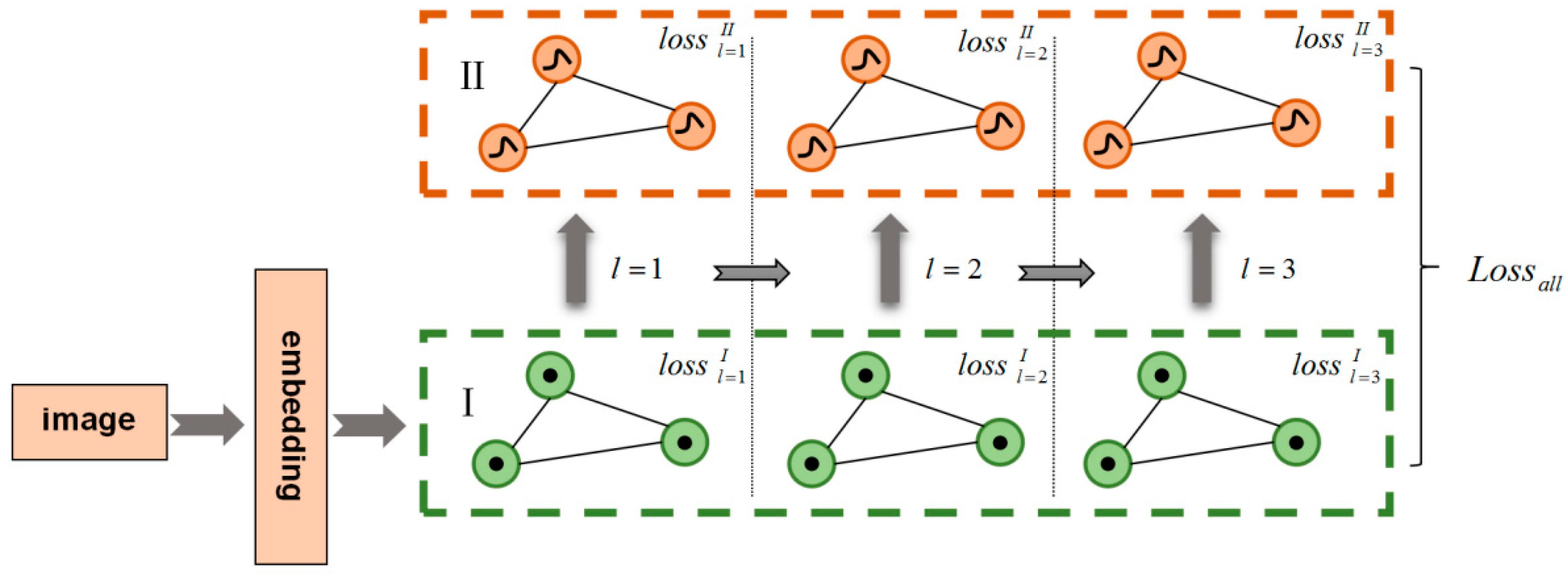
3. Edge-Weight Single-Step Memory-Constraint Network (ESMC)

3.1. N-Way K-Shot Mode

The N-way k-shot problem is a classification problem that often occurs in the field of few-shot and meta-learning, where n is the number of categories sampled, and K is the number of samples randomly sampled in each category. In the face of few-shot classification, we borrow other existing rich label datasets to help with classification. In the base class, we continuously construct small classification tasks through random sampling of rich label datasets and overlay training to realize the generalization of the model [43,44]. In the novel class, we realize the real few-shot classification, learn in the same mode before and after, and realize the subsequent classification in the novel class through continuous learning in the constructed classification task. In one task, after sampling from the novel class, a novel support set ($S_n$) and novel query set ($Q_n$) are formed. In the base class, a base support set ($S_b$) and base query set ($Q_b$) are also constructed with the same number of samples. In the whole task, the key to determining N and K is to look at the sampling situation in the meta-testing stage. Therefore, to determine the number of N and K, we need to judge by the sampling situation in the meta-testing stage. Generally, the value is determined according to the data distribution of the support set part. Meta-testing and meta-training always maintain the same sampling method and are similar in the construction of classification tasks. When comparing the accuracy, various experiments in the field of few-shot classification often use 5-way–1-shot and 5-way–5-shot to train, test, compare, and analyze the accuracy of these two models [45].

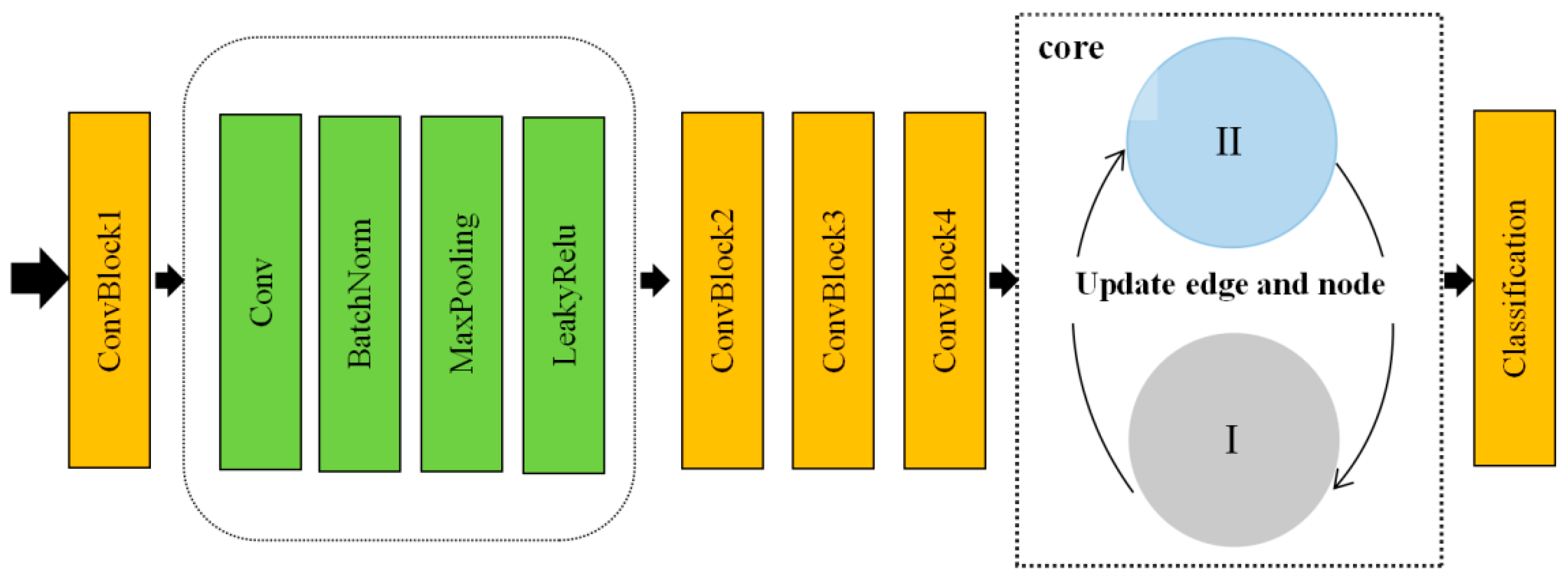
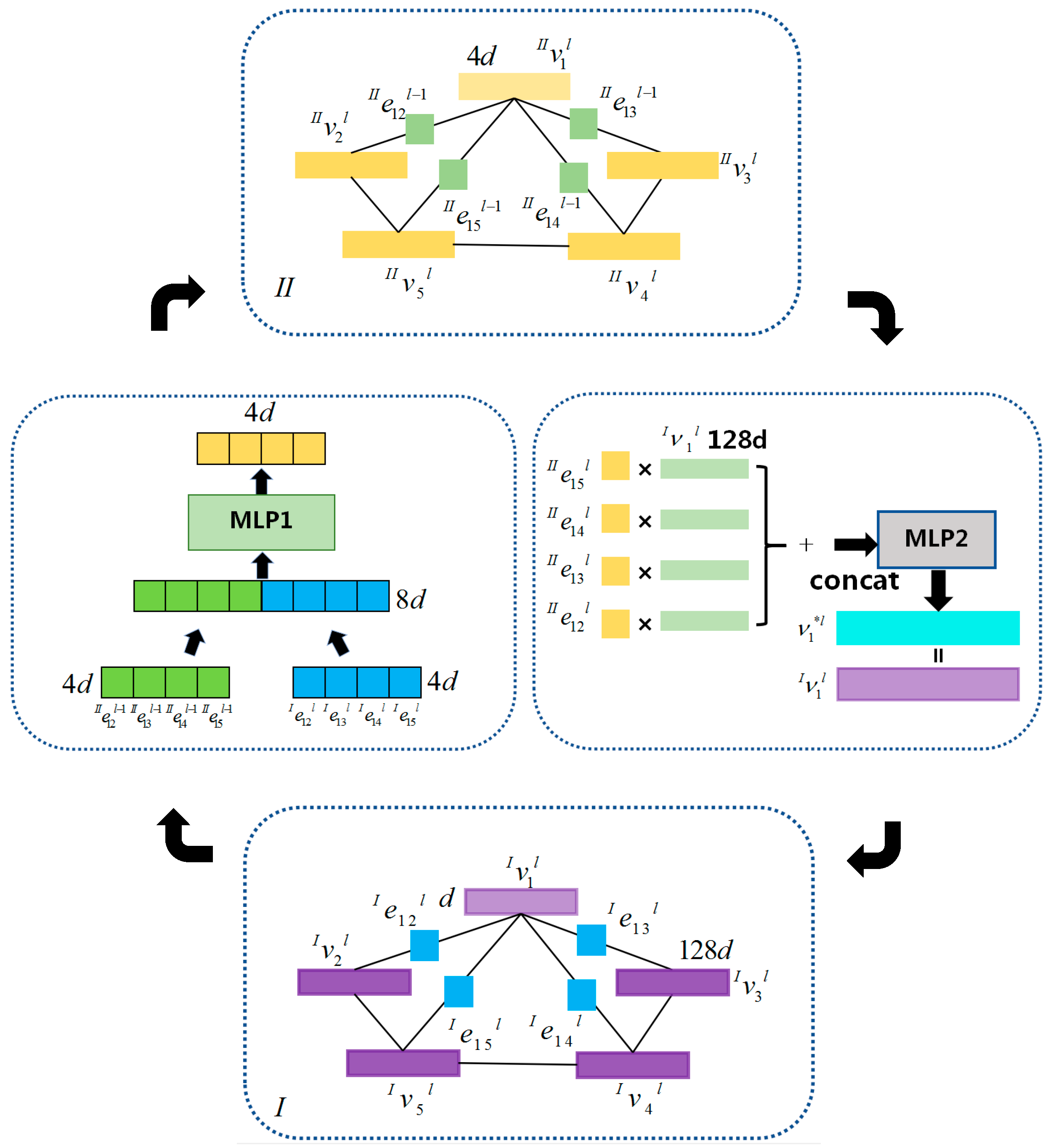
3.2. Graph Neural Network

As shown in Figure 2, an ESMC flow diagram is mainly divided into four parts: Zone I based on node features graph structure, Zone II based on edge-weight data, Zone I to II transition module (mosaic of Zone I and II edge-weight features and node update of Zone II) and Zone II to I transition module (mainly realizing the fusion of Zone II edge and Zone I node features). In order to simplify the expression of the network process, this section mainly takes the support set samples in 5-way–1-shot as an example, and the samples in the query set section also use the same calculation.

Figure 2. Schematic diagram of ESMC.

3.2.1. Edge Initialization and Update of the Graph Structure in Zone I

In Figure 2, Zone I is the graph structure of the EGNN network based on node features. A general GNN is a graph directly connecting all nodes from the support set to the query set. Nodes classify the query set’s samples by using the embedding vector and the single-heat encoding label representation and by iteratively updating the node features through neighbor aggregation. Considering that the method of explicit edge annotation is to assign the initial edge weight to the edges directly, this practice also combines representation learning and measurement learning, which can enable the information between nodes and edges to be fully utilized.

The initial edge weights are set as follows:

$$\begin{gathered} y_{ij}=\{\begin{array}{cc}1,& if\begin{array}{c}{y}_i=y_j\end{array}\\ 0,& otherwise.\end{array}\begin{array}{cc}& i,j\le N\end{array} \\ {}^{(I)}e{}_{ij}^0=\{\begin{array}{cc}[1||0],& if\begin{array}{c}{y}_{ij}=1\begin{array}{c}\end{array}\end{array}\\ [0||1],& if\begin{array}{c}{y}_{ij}=0\begin{array}{c}\end{array}\end{array}\\ [0.5||0.5],& otherwise.\end{array}\begin{array}{cc}& i,j\le N\end{array} \end{gathered}$$

(1)

where $i,j$ is the image sample mark of Zone I, $N$ is the total number of samples of a task, and $y_i,y_j$ is the label of the real category of the sample—if 1, it is similar; if 0, it is alien. Set the initial edge ${}^{(I)}e{}_{ij}^0$ weight of Zone I according to the judgment result of $y_{ij}$. ${}^{(I)}e{}_{ij}^0$ is composed [internal similarity || phase difference between classes]. For the unknown category samples, the initial value is 0.5, and the other value is 0 or 1.

The Zone I edge-weight update, as shown in Figure 3, is as follows. First, the feature node ${}^{I}v{}_1^l$ is calculated by its other adjacent nodes ${}^{I}v{}_2^l,{}^{I}v{}_3^l,{}^{I}v{}_4^l,{}^{I}v{}_5^l$, and then the resulting vector is sent into MLP3. MLP3 is mainly composed of dimension reduction, convolution, BN, LeakyReLU, and Dropout operations. After a series of similarity calculations, the current layer $l$ ($l\in [1,3]$) gets one-dimensional similarity calculation results multiplied by the $l-1$ layer edge weight to update the edge weight.

Figure 3. Schematic diagram of updating the border rights in Zone I.

The general formula for weight updates in this phase is as follows:

$$\begin{gathered} {}^{I}e{}_{ij1}^l=\frac{{}^{(I)}f{}_e^l({}^{I}v{}_i^l,{}^{I}v{}_j^l;{\theta }_e^l){}^{I}e{}_{ij1}^{l-1}}{{\displaystyle {\sum }_k{}^{(I)}f{}_e^l({}^{I}v{}_i^l,{}^{I}v{}_k^l;{\theta }_e^l){}^{I}e{}_{ik1}^{l-1}/({\displaystyle {\sum }_k{}^{I}e{}_{ik1}^{l-1})}}}, \\ {}^{I}e{}_{ij2}^l=\frac{(1-{}^{(I)}f{}_e^l({}^{I}v{}_i^l,{}^{I}v{}_j^l;{\theta }_e^l)){}^{I}e{}_{ij2}^{l-1}}{{\displaystyle {\sum }_k(1-{}^{I}f{}_e^l({}^{I}v{}_i^l,{}^{I}v{}_k^l;{\theta }_e^l)){}^{I}e{}_{ik2}^{l-1}/({\displaystyle {\sum }_k{}^{I}e{}_{ik1}^{l-1})}}}, \\ {}^{I}e{}_{ij}^l={}^{I}e{}_{ijd}^l/{\Vert {}^{I}e{}_{ijd}^l\Vert }_1 \end{gathered}$$

(2)

where ${}^{(I)}f{}_e^l$ is the edge-weight update similarity calculation function, ${}^{I}v{}_i,{}^{I}v{}_j$ is the Zone I node, ${\theta }_e^l$ is the set of parameters, $k$ is all node marks, $k\in [0,N]$, ${}^{I}e{}_{ij2}^l$ and ${}^{I}e{}_{ij1}^l$ are the updated edge weights, representing the intra-class similarity and inter-class phase specificity, respectively, $d$ are 1, 2, generally, the sum is set to 1.

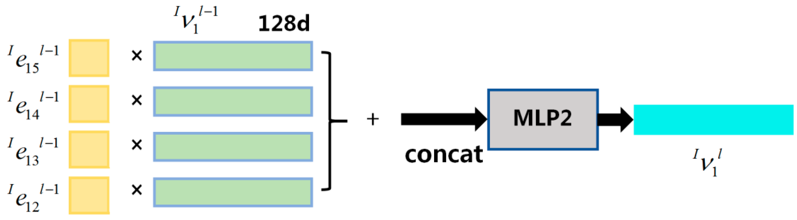
3.2.2. Node Initialization and Update of the Graph Structure in Zone I

In contrast to the custom method for calculating the initial edge weight in Zone I, the initialized node features of Zone I are obtained through model learning in the network with an embedding layer especially used to extract the initial node features. The updating of the node features in the graph structure is different from its initial node features. The two parts exist as mutually independent modules. The updated schematic diagram of the Zone I node is shown in a diagram structure in Figure 4. The main operation mode of the update of ${}^{I}v{}_1^{l-1}$ is actually the same as the module operation obtained by $v^{*}{}_1^l$ in Figure 2. First, it is necessary to multiply and sum ${}^{I}v{}_1^{l-1}$ with the edge weight ${}^{I}e{}_{12}^{l-1},{}^{I}e{}_{13}^{l-1},{}^{I}e{}_{14}^{l-1},{}^{I}e{}_{15}^{l-1}$ connected to this node, then perform the splicing operation, and finally enter MLP2. The main operations implemented in MLP2 are convolution, BN, LeakyReLU, and Dropout, thus obtaining the new node feature ${}^{I}v{}_1^l$ of $l$ layer in Zone I.

Figure 4. Schematic diagram of node-feature update in Zone I.

The general formula for the initial node update is as follows:

$$\begin{gathered} v_i^0={}^{(I)}f{}_{emb}(x_i;{\theta }_{emb}) \\ {}^{I}v{}_i^l={}^{(I)}f{}_v^l([{\displaystyle \sum _j{}^{I}e{}_{ij1}^{l-1}{}^{I}v{}_j^{l-1}||{\displaystyle \sum _j{}^{I}e{}_{ij2}^{l-1}{}^{I}v{}_j^{l-1}}}];{\theta }_v^l) \end{gathered}$$

(3)

where ${}^{(I)}f{}_{emb}$ is the convolutional mapping function, ${\theta }_{emb}$ is the set of parameters, ${}^{(I)}f{}_v^l$ is the $l$ layer node transmission network. ${}^{I}v{}_i^l$ is the characteristic of the $i$ sample of the $l$ layer, $v_i^0$ is the initial node feature, and $x_i$ is the $i$ sample.

3.2.3. Edge Initialization of the Edge Weights Structure in Zone II

When $l=1$, Zone I graph networks $v_i^0$ and $e_{ij}^0$ are updated, if, according to the previous way of doing 2–3 layers of updating, the network is still mainly updated node features, and ignoring the important implicit information in the data-distribution level. In particular, the data distribution of ${}^{I}e{}_{ij}^l$ at the edge of Zone I implies that information also represents a “special” multidimensional feature composed of ${}^{I}e{}_{ij}^l$. This abstract feature comes from the intra-class similarity and inter-class dissimilarity between the sample image features.

Therefore, to better combine node features representing the sample instances with edge features representing the sample distribution, a one-step memory-constraint network builds a graph structure based on the characteristics of the edge-weight distribution. In this process, Zone II also adopts the same initial edge-weight setting rules as Zone I. First, it is necessary to judge the same class of the sample. This part is mainly based on the edge-weight distribution, so it is necessary to find the corresponding nodes according to the current edge-weight characteristics and then set the initial edge label according to the judgment results.

The initial edge weights used in Zone II are set as follows:

$$\begin{gathered} y_{mn}=\{\begin{array}{cc}1,& if\begin{array}{c}{y}_m=y_n\end{array}\\ 0,& otherwise.\end{array}\begin{array}{cc}& m,n\le N\end{array} \\ {}^{(II)}e{}_{mn}^0=\{\begin{array}{cc}0& if\begin{array}{c}{y}_m\ne y_n,\end{array}\\ 1& if\begin{array}{c}{y}_m=y_n\begin{array}{c}\end{array},\end{array}\\ 0.5& otherwise.\end{array}\begin{array}{cc}& m,n\le N\end{array} \end{gathered}$$

(4)

where $m,n$ is the sample mark of Zone II. $y_m,y_n$ is the real class label of the node corresponding to the multidimensional edge-weight feature, ${}^{(II)}e{}_{mn}^0$ is the initial edge label, and $N$ is the total number of samples for a task.

3.2.4. Node Update of the Edge-Weight Implicit Distribution Graph Structure in Zone II

When $l$ > 0, as shown in Figure 2, by stitching the edge data ${}^{I}e{}_{12}^l,{}^{I}e{}_{13}^l,{}^{I}e{}_{14}^l,{}^{I}e{}_{15}^l$ of Zone I and the edge data ${}^{II}e{}_{12}^{l-1},{}^{II}e{}_{13}^{l-1},{}^{II}e{}_{14}^{l-1},{}^{II}e{}_{15}^{l-1}$ of $l-1$ layer in Zone II, to structure a vector of 8d, the number of channels remains unchanged, the feature dimension increases, and it is a one-way feature fusion, which is the so-called single step.

This part of the graph structure is always splicing ${}^{II}e{}_{12}^{l-1},{}^{II}e{}_{13}^{l-1},{}^{II}e{}_{14}^{l-1},{}^{II}e{}_{15}^{l-1}$ of the Zone II $l-1$ layer to retain the previous edge-weight data-distribution characteristics and constantly remembers the upper edge-weight information in one way, which is a memory constraint.

Then, after MLP1, this part is mainly operated as FC and LeakyReLU to fuse the feature vector dimension reduction into 4d size and to increase the data nonlinearity so as to restrain the formation of a new feature information and then as the node of the new Zone II graph structure. Its node update formula is as follows:

$${}^{II}v{}_m^l={}^{(II)}f{}_{emb}([{}^{II}e{}_{ij}^l\left|\right|{}^{II}e{}_{mn}^{l-1}];{\phi }_{emb})$$

(5)

where ${}^{(II)}f{}_{emb}$ is the mapping function of the obtained Zone II nodes. ${\phi }_{emb}$ is a set of parameters for a node update network. ${}^{II}v{}_m^l$ is the $m$ node feature of $l$ layer, where || is the concat operation.

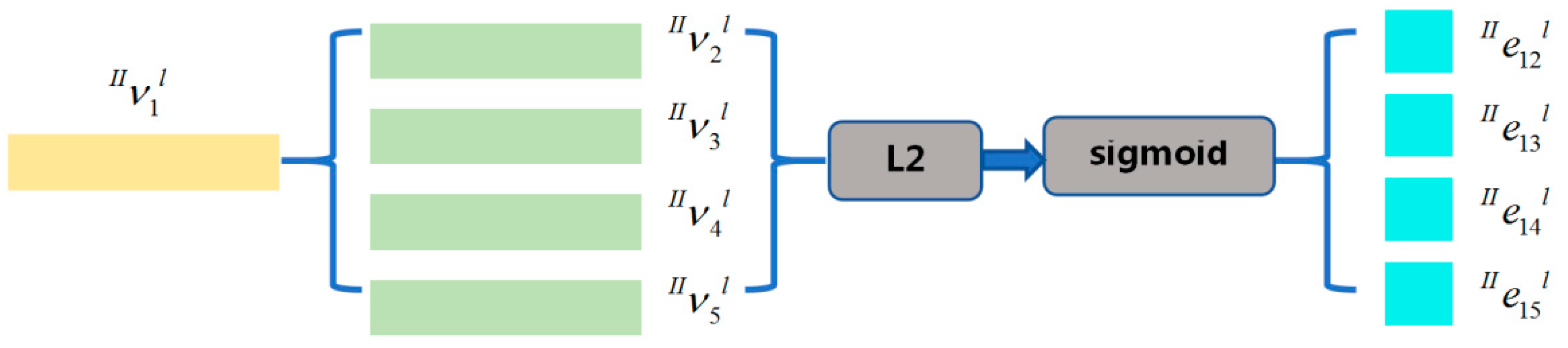
3.2.5. Edge Update of the Edge-Weight Implied Distribution Graph Structure Zone II

The update of the edge weights in the Zone II graph structure is shown in Figure 5. First, it is necessary to calculate the L2 distance between the ${}^{II}v{}_1^l$ of the $l$ layer and the other nodes ${}^{II}v{}_2^l,{}^{II}v{}_3^l,{}^{II}v{}_4^l,{}^{II}v{}_5^l$ in Zone II and then to normalize the resulting similarity measure result between 0 and 1 through the Sigmoid function to get the final edge-weight update result.

Figure 5. Schematic diagram of renewal of border rights in Zone II.

When $l>0$, to reduce the risk of overfitting the few-shot, a relatively simple method is adopted to calculate the edge weight of the Zone II graph structure. This paper mainly uses L2 distance. The smaller, the higher the similarity, and the larger the distance, the lower the similarity. Its general update formula is as follows:

$${}^{II}e{}_{mn}^l={}^{(II)}f{}_e^l({({}^{II}v{}_m^l-{}^{II}v{}_n^l)}^2;{\phi }_e^l)$$

(6)

Among them, ${}^{II}e{}_{mn}^l$ is the edge weight between $m$ and $n$ node nodes in the $l$ layer, ${}^{(II)}f{}_e^l$ is the $l$ layer edge-weight update similarity calculation function, ${\phi }_e^l$ is the set of parameters, ${}^{II}v{}_m^l$ is the $m$ node feature of the $l$ layer, and ${}^{II}v{}_n^l$ is the $n$ node feature in the $l$ layer. This ${}^{II}e{}_{mn}^l$ is not the final result and also requires normalization ${}^{II}e{}_{mn}^l$ in practical application.

3.2.6. Feature Fusion Update of Zone II and Zone I

The transition from Zone II to Zone I, as shown in Figure 2, better integrates the node features of the junction between Zone I and Zone II edge features, i.e., integrates the resulting edge-weight hidden features into the node features. The updated ${}^{II}e{}_{12}^l,{}^{II}e{}_{13}^l,{}^{II}e{}_{14}^l,{}^{II}e{}_{15}^l$ in Zone II requires feature mapping through function $f_v^l$, and considers the intra-node class similarity and phase specificity between classes. Then, through MLP2, this part is mainly convolution, BN, LeakyReLU, and Dropout. This enables the update ${}^{I}v{}_1^l$ node in $l$ of the current Zone I layer. This section updates the formula group as follows:

$$\begin{gathered} v^{*}{}_i^l=f_{v^{*}}^l([{\displaystyle \sum _i{}^{II}e{}_{mn}^l{}^{I}v{}_i^l||{\displaystyle \sum _i\sum 1-{}^{II}e{}_{mn}^l)\cdot {}^{I}v{}_i^l}}];{\theta }_{v^{*}}^l) \\ {}^{I}v{}_i^l=v^{*}{}_i^l \end{gathered}$$

(7)

Among them, $m,n,i\le N$, $f_{v^{*}}^l$ is the node similarity calculation function of the $l$ layer from Zone II to Zone I, ${\theta }_{v^{*}}^l$ is the set of parameters, $v_i^{*l}$ is the result of the fusion of the characteristics of Zone II and Zone I of the current layer $l$, and ${}^{I}v{}_i^l$ is the feature vector of the $i$ node in Zone I.

Through the introduction of the above module process, we can find that the update function and Formula (7) in many places are the same, but there are different details. The difference is ${}^{I}e{}_{ij}^l$, which is used in Formula (3) for the Zone I edge-weight features. Each edge represents the similarity between instances (points), namely the similarity between the sample nodes. The edge-weight feature ${}^{II}e{}_{mn}^l$ of Zone II is used in Equation (7). After the Euclidean distance calculation and normalization, each edge represents the similarity between the distributions (edges), which is the implied distribution feature of the edge-weight data. Thus, after a round of learning of all the data, the edge nodes of Zone I and II are updated, the graph structure of the two parts is complete, and the operation of the next layer begins.

3.2.7. Loss Function

In the one-step memory-constraint network structure, there are three layers of loop updates that are set. $l=[1,3]$ when $l=0$ is the initialization layer. As shown in Figure 6 below, in one loop, the edge-weight prediction value for both Edge 1 and Edge 2 will respectively be obtained in Zones I to II, and the second dimension of each vector is 3 because the dimension represents the number of loop layers of the graph network. Each layer gets two edge-weight prediction results. When calculating the accuracy, the last layer of edge-weight update value in Zone I is used.

Figure 6. ESMC loss composition diagram.

In calculating the loss with BCE, the prediction results for each layer and each region are adopted to make the optimization effect more accurate. The setting formulas and parameters of Zone I and II are similar, as follows:

$${}^{(I)}L=0.5\cdot L_{BCE}^{l=1}(pr\_e1,target)+0.5\cdot L_{BCE}^{l=2}(pr\_e1,target)+L_{BCE}^{l=3}(pr\_e1,target)$$

(8)

$${}^{(II)}L=0.5\cdot L_{BCE}^{l=1}(pr\_e2,target)+0.5\cdot L_{BCE}^{l=2}(pr\_e2,target)+L_{BCE}^{l=3}(pr\_e2,target)$$

(9)

where $pr\_e1$ and $pr\_e2$ is the edge-weight prediction result of the two Zones; ${}^{(I)}L$ is the loss of Zone I, and ${}^{(II)}L$ is the loss of Zone II. In a three-layer cycle, the loss weights are 0.5, 0.5, and 1.

The first two layers are mainly used as auxiliary learning layers, and the last layer is used as the most important layer for accuracy calculation, so the weight proportion is the largest. Therefore, the loss calculation formula of the one-step memory-constraint network, which ultimately needs to conduct backpropagation, is as follows:

$$L_{all}={}^{(I)}L+0.1{}^{(II)}L$$

(10)

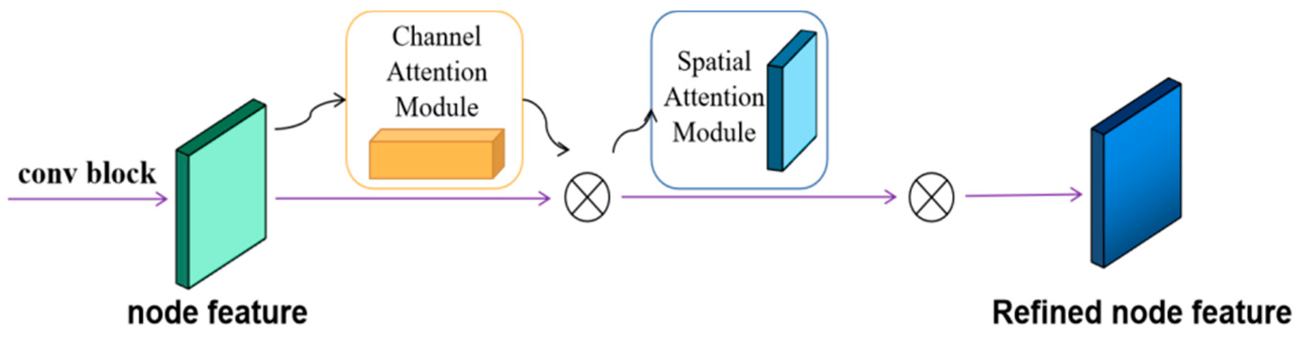
3.3. Feature Extraction of the Initialized Nodes Based on Attention

The ESMC mainly explores hidden feature information to realize new distribution-level feature learning. Every time random sampling constitutes a classification task, the first work to be done is the feature extraction of the image samples, i.e., initial node-feature extraction [46]. If initial feature extraction is not good enough, this is influential for all subsequent updates. This subsection describes the improvement of the attention mechanism on the initial feature extraction effect.

Figure 7 is the overall framework diagram of the convolutional block attention mechanism. The general use order is to first use the channel attention to input the feature map obtained from the channel attention module into the spatial attention module so as to gradually realize the feature attention on the channel and the image space. This process corresponds to the model in adaptively adjusting the local attention of the image. The CBAM is a lightweight and easily integrated module that can be used in many convolutional networks [47], along with end-to-end training. Its two-part attention module can be used for plug-and-play and can also be used selectively, easily, and simply when integrated into the existing network architecture.

Figure 7. Convolutional Block Attention Mechanism (CBAM).

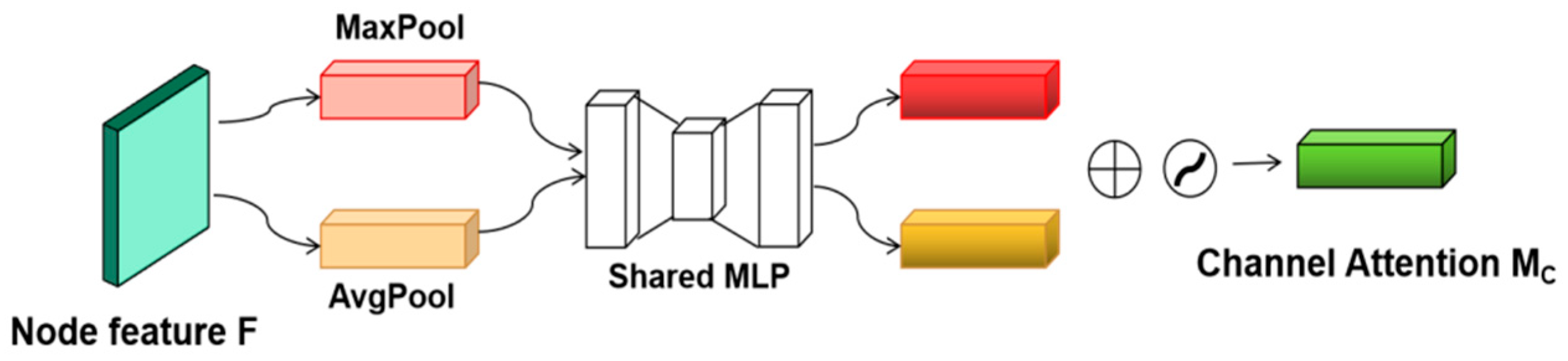
3.3.1. Initialized Node-Feature Extraction Based on Channel Attention

In the channel attention module, as shown in Figure 8, in the process of image extraction, multiple channels are often used to obtain features in different situations. Model learning assigns different weights to different channels to extract useful features so as to obtain meaningful sample features based on the channel [48]. In this attention module, global average pooling and global maximum pooling are only used to achieve attention, summarizing the features of the channel.

Figure 8. Channel attention in convolutional block attention module.

As shown in the figure, the operation in the channel attention module first passes the input feature map $\mathrm{F}$ through global max pooling and global average pooling based on height and width, then passes through MLP operation, obtains new features through convolution, dimensionality reduction, etc., adds the output features element by element at the corresponding position, and then gets the final feature map under the channel attention mechanism through Sigmoid activation.

Subsequently, we need to integrate the feature map and the original input feature map and multiply element by element at the corresponding positions so as to get the subsequent input feature map into the spatial attention module. The calculation formula is as follows:

$$\begin{array}{l}{\mathrm{M}}_{\mathrm{c}}(\mathrm{F})=\sigma (MLP(AvgPool(\mathrm{F}))+MLP(MaxPool(\mathrm{F})))\\ \begin{array}{cc}& \begin{array}{cc}& =\sigma ({\mathrm{W}}_1({\mathrm{W}}_0({\mathrm{F}}_{\mathrm{avg}}^{\mathrm{c}}))+{\mathrm{W}}_1({\mathrm{W}}_0({\mathrm{F}}_{\max }^{\mathrm{c}})))\end{array}\end{array}\end{array}$$

(11)

where $W_0\in R^{C/r\times C}$, $W_1\in R^{C\times C/r}$, $\sigma$ is the Sigmoid operation, $r$ is the reduction rate, $W_0$ followed by the ReLU nonlinear activation.

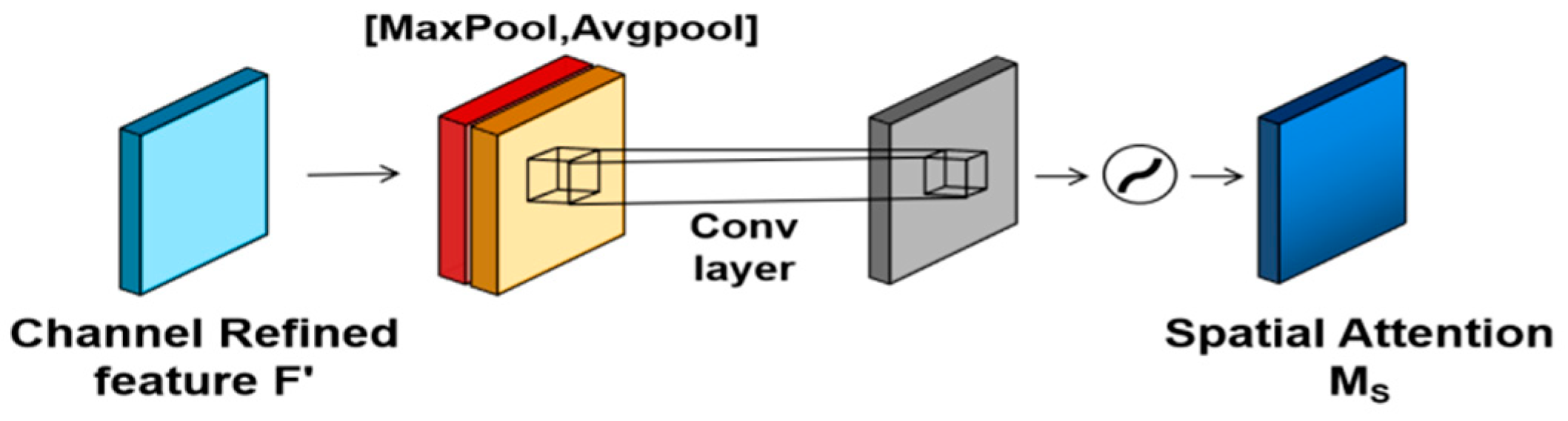
3.3.2. Initialized Node-Feature Extraction Based on Spatial Attention

The spatial attention module is slightly different from the channel attention module in the whole mind. As can be seen from the name, one focuses on the channel, and the other focuses on the space. Channel attention is based on the weight obtained on the channel dimension, while spatial attention is based on the spatial dimension obtained from the characterization of the features of various parts of an image, as shown in Figure 9, which is the framework diagram of the spatial attention module.

Figure 9. Spatial attention in convolutional block attention module.

The function of the spatial attention module can be clearly seen in Figure 9. It is based on the maximum pooling and average pooling of one channel dimension, and then the channel descriptions of the two pooling operations are fused through convolution [49]. Then, through a $7\times 7$ further convolution layer, using the activation function Sigmoid, the feature graph of that phase is multiplied by the original feature graph to get the new feature graph. Generally, the input of the spatial attention module is the output of the channel attention module, but a feature $\mathrm{F}$ with $H\times W\times C$ can also be given according to the different embedding methods. After obtaining the weight coefficient ${\mathrm{M}}_s(\mathrm{F})$ of the image, the output can be obtained by multiplying the output with the original image. The calculation principle is shown in Formula (12).

$$\begin{array}{l}{\mathrm{M}}_s(\mathrm{F})=\sigma (f^{7\times 7}([AvgPool(\mathrm{F});MaxPool(\mathrm{F})]))\\ \begin{array}{cc}& \begin{array}{cc}& =\sigma (f^{7\times 7}([{\mathrm{F}}_{avg}^s;{\mathrm{F}}_{\max }^s]))\end{array}\end{array}\end{array}$$

(12)

where $\sigma$ is the Sigmoid nonlinear activation operation, $7\times 7$ represents the size of the convolutional kernel. The convolution kernel of $7\times 7$ is better than that of $3\times 3$.

In actual use, CBAM integration into the network has a variety of methods. The most common is Conv Block. We can also not change the network structure; it is only added in the first layer and the last layer. At the same time, we can also use channel attention and spatial attention separately. Different integration strategies will generate different effects.

4. Experimental Results and Analysis

Relevant experiments were performed on the miniImageNet dataset. Firstly, the relevant configuration parameters are introduced. On the basis of ESMC, the influence of 5-way 1-shot and 5-way–5-shot was analyzed, and relevant discussion and analysis was conducted.

4.1. Parameters Setting

Datasets: MiniImageNet [17] is the standard dataset in the few-shot field, containing 100 categories, including 600 samples and 600,000 color pictures. Each picture specification is $84\times 84$, the picture is a single label, and the target occupies a large zone in the whole image. There is no need for a preprocessing operation. The ratio of the training set to the prediction set is 8:2. In the experiment reported in this section, a set of evaluation criteria is provided for this dataset, namely average accuracy (mean acc), on which it is trained and tested. The example images of the dataset are shown in Figure 10.

Figure 10. The example images of the dataset.

Training: There are two model training modes: 5-way 1-shot and 5-way 5-shot. Samples in each task were sampled randomly. The model used the Adam method to optimize the network parameters. The batch size was set to 40. The learning rate was set to exponential decay. The original learning rate per 15,000 generations was set to 0.99 times. The initialized learning rate was set to 0.001. We stopped the training of the entire dataset at 100,000 generations (Epoch). To prevent the model from overfitting, we set the random deactivation rate (Dropout) to 0.1. A regularization term with a weight decay rate (Weight decay) of 1 × 10⁻⁶ was also set.

4.2. Experimental Results

4.2.1. Impact of ESMC on Classification Performance

The processes and the setting of the losses of ESMC are shown in Figure 2. During the transition from Zone I to Zone II, the feature-splicing part always adopts the Zone II graph edge weight of the $l-1$ layer. Moreover, this practice of increasing feature richness is very similar to memorizing data information in the upper layer. In contrast to bidirectional LSTM and forward and reverse acquisition of bidirectional features, the memory of ESMC belongs to the $l-1$ layer and to the $l$ layer and one-way memory, which is also the reason it is called single-step. In addition, this memory-splicing method enlarges the feature information of the edge-weight distribution level of Zone II so that the network can take into account the data information of Zone II when learning the characteristics of Zone I, thus realizing the so-called memory-constraint network.

The experiment in this paper is currently based on two modes, 5-way 1-shot and 5-way 5-shot. Since the samples in the dataset are pickel files and multiple coded data after reading, the classification results of images can not be directly visualized, so the accuracy of the experimental results is expressed by mean acc. Moreover, the few-shot classification network is different from the general convolutional neural network. Its training and testing methods were introduced in the second section, and the sample categories of training and testing are completely disjointed. After adding the edge-weight one-step memory-constraint module, the average accuracy results obtained by both modes were improved. As shown in the 5-way 1-shot mode in Table 1, our method achieves a relatively good effect, which is higher than the ESNN [11] methods, MatchingNet [17], wDAE [20], RelationNet [22], Meta-Transfer [24], TPN [36], R2D2 [38], MAML [39], Dynamic [40], GNN [41], Global [43], CloserLook [50], respectively. After adding the edge-weight feature measure, EGNN adds more abundant feature information on the basis of the original network. There are also the characteristics of implicit edge-weight distribution in Zone II. So, from a cardinal point of view, ESMC does a good job of helping graph neural networks learn more data. In the 5-way–5-shot mode, the proposed ESMC makes the feature information rich and makes full use of the correlation of only samples. At the same time, the setting rules of initial edge weights are closer to the real category of samples, and the consideration of network details is more careful. Thus, it also improves the effect of final classification by at least 1.16% compared with other mainstream models.

Table 1. The influence of ESMC on classification performance.

Method	Backbone	5 Way-1 Shot (%)	5 Way-5 Shot (%)
MatchingNet	ConvNet	43.56 ± 0.84	55.31 ± 0.73
ProtoNet	ConvNet	49.42 ± 0.86	68.20 ± 0.54
RelationNet	ConvNet	50.44 ± 0.82	65.32 ± 0.70
R2D2	ConvNet	51.20 ± 0.78	68.20 ± 0.61
MAML	ConvNet	48.70 ± 1.84	63.11 ± 0.92
Dynamic	ConvNet	56.20 ± 0.86	71.94 ± 0.62
GNN	ConvNet	50.33 ± 0.36	66.41 ± 0.63
TPN	ConvNet	55.51 ± 0.93	69.86 ± 0.78
Global	ConvNet	53.21 ± 0.89	72.34 ± 0.74
wDAE	WRN	61.07 ± 0.15	76.75 ± 0.11
CloserLook	Resnet18	51.75 ± 0.83	74.59 ± 0.64
Meta-Transfer	ResNet12	61.20 ± 1.8	75.53 ± 0.80
EGNN	ConvNet	59.14 ± 0.71	76.37 ± 0.60
ESMC(ours)	ConvNet	65.97 ± 0.69	77.46 ± 0.44

The first reason for this is that the EGNN itself does not make rich use of the feature information of the constructed graph network when it processes a small amount of data. Therefore, the 5-way 1-shot experiment resulting in the EGNN network is not as accurate as other experiments in the same period; secondly, the ESMC causes the features of the data-distribution level to be learned continuously. For each task alone, $l=[1,3]$, each batch size is 40 for 100,000 generations, which is enough to accumulate the huge training amount and enrich the self-learning content, thus achieving a better classification effect.

For the 5-way 5-shot model, accuracy was also improved by 1.16%. The index improvement is not as large as the 5-way 1-shot model, probably because, first, in a task, the sample size of the 5-way–5-shot model is three times that of the 5-way–1-shot, so the added edge-weight distribution feature information can only be partially added to the original sufficient information, so the effect may not be as obvious as the 5-way–1-shot model. For the newly improved network, to more intuitively observe the clustering effect of nodes, we visualized the node features of each layer, as shown in Figure 11, showing the effect of the TSNE visualization of node features in a 5-way–5-shot model, mainly to realize the high-dimensional clustering of node features in a more intuitive way compared to the abstract multidimensional features.

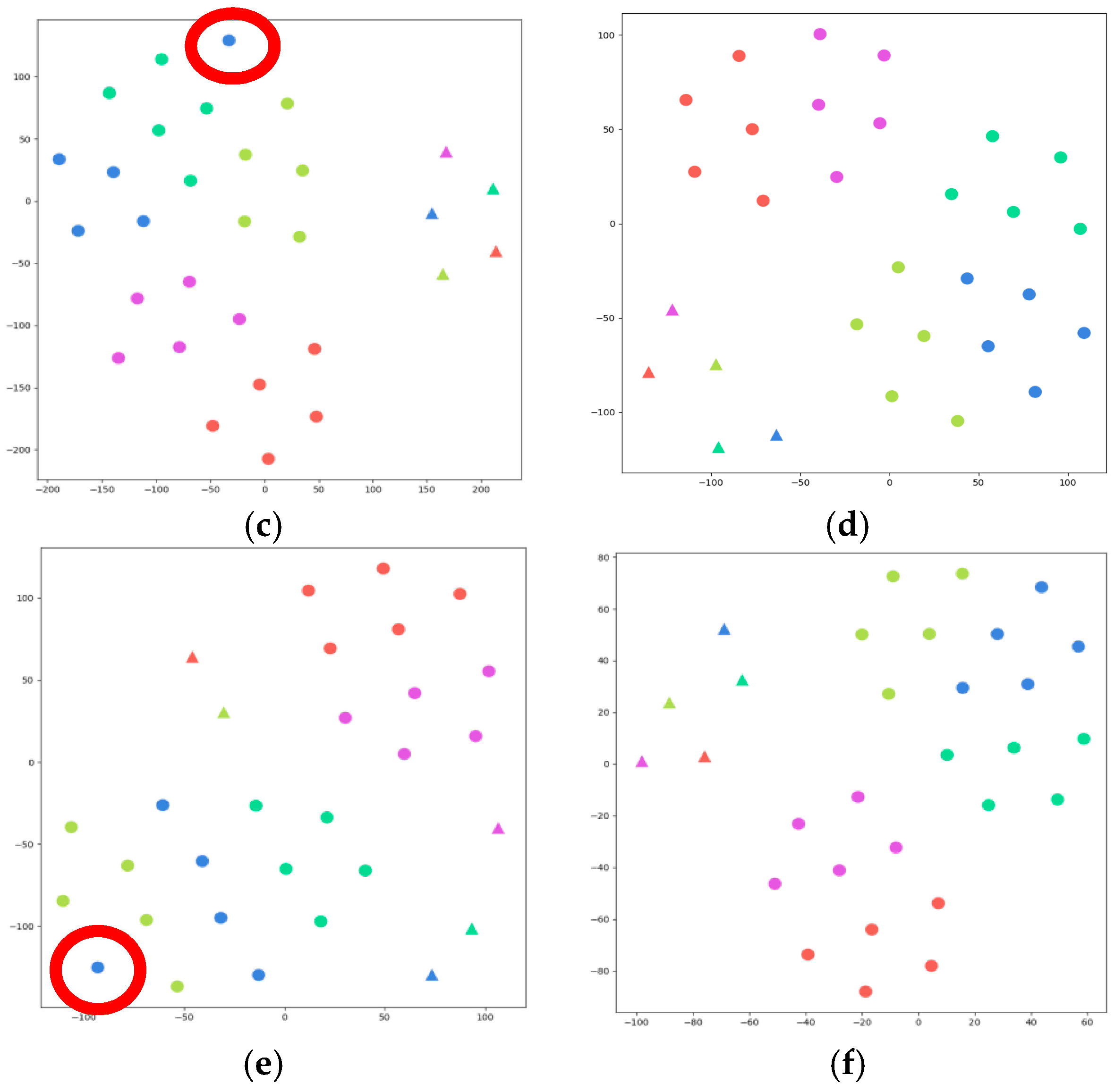
Figure 11. The visualization of the TSNE node features. (a) Visualization of the EGNN $l=1$ layer node features. (b) No feature visualization of the ESMC $l=1$ layer. (c) EGNN $l=2$ layer node feature visualization. (d) ESMC $l=2$ layer node feature visualization. (e) EGNN $l=3$ layer node feature visualization. (f) ESMC $l=3$ layer node feature visualization. ““ represents the samples of query set, and “” represents the samples of suppport set. Different colors represent different categories. The samples in the red circle are the samples that were shifted during clustering.

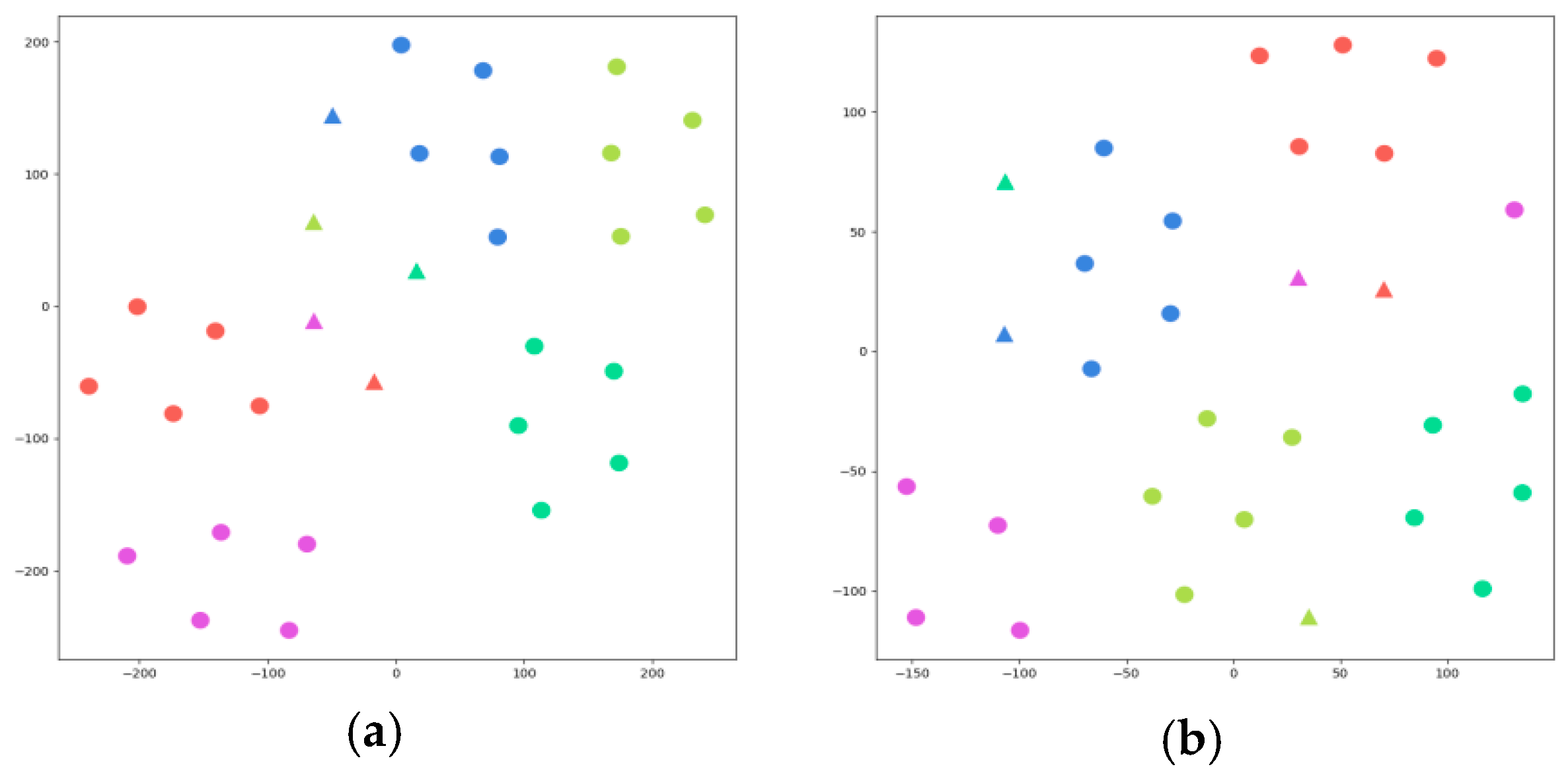
In the experiment, the confusion value is 20, the order from top to bottom in the graph is $l=1$, $l=2$, $l=3$, from left to right is EGNN, and in the left-to-right single-step memory-constraint network (ESMC), the triangle represents the sample of query set, and the circle represents the sample of suppport set.

From the detailed analysis of the distribution of the scatter plot, we can find that EGNN also shows better results in the clustering of sample features. As with the edge-weight one-step memory-constraint network, when $l=1$, there are some sample distribution errors, but the EGNN is still confused at $l=2$ and $l=3$, and all the scatter points do not achieve the optimal clustering effect. In fact, in the state where the node features are constantly updated, the best result we expect is to ensure that node features obtained after the update of each layer can become more and more obvious and the obtained clustering effect is getting better and better, i.e., various kinds of samples can cluster more obviously and do not interfere with each other.

Through alignment analysis, the edge-weight one-step memory-constraint network outperforms the EGNN network in the final performance. In the graph with layer $l=2$, $l=3$, the sample clustering division is obvious, and there is no special error scatter, which is closer to the ideal distribution state. Therefore, we can also verify that the improved ESMC has a relatively good node-feature extraction ability, and the performance of node aggregation can also reflect that the interdependent edge-weight features should also have a good extraction effect.

After the visualization of node features, to more intuitively show the change of edge weight, the ESMC edge-weight features are also visualized. Unlike the high-dimensional features of nodes, edge weight is a kind of feature vector similar to the correlation matrix, which is a two-dimensional feature.

In the experiment, the edge-weight view under the real label, the initialized edge-weight view, and the $l=1$, $l=2$, $l=3$ layer of the graph network are given. By converting the edge-weight value into color blocks, it is clear how the evolution trend of the whole color block is constantly updated by edge weights gradually close to the real label.

In Figure 12, the deepest color block is $e_{ij}$ = 1, which means that the probability that the two samples $i$ and $j$ has to belong to the same class is 1, and the white color block is $e_{ij}=0$, indicating that the two samples $i$ and $j$ cannot belong to the same class as the two samples. From deep to shallow represents a decrease in correlation between samples. Figure 12 shows the visualization results of the real label features connecting the edge weights between the samples in the few-shot five-classification task 5-way 1-shot. Until the last layer of the edge-weight feature visualization (Figure 13d), its color block distribution is increasingly similar to the edge-weight real label visualization diagram. In this part of the experiment, we used the experimental results under the 5-way–1-shot model. The first 5 rows are the association degree of support set samples with other samples, and the last 5 rows are the correlation degree of query set samples with other samples.

Figure 12. ESMC visualization of edge-weight real label features.

Figure 13. Edge-weight feature visualization. (a) ESMC initializes edge-weight feature visualization. (b) ESMC $l=1$ edge-weight feature visualization. (c) ESMC $l=2$ edge-weight feature visualization. (d) ESMC $l=3$ edge-weight feature visualization.

Ideally, we want to make the edge-weight visual color block of the $l=3$ layer similar to the real label map, i.e., the diagonal is all dark, and the other parts are all white. The above images clearly show the representation effect of the edge weights after constant updates. Although there are still less-than-ideal color blocks in the last visual layer, the overall color block remains at a good level. The color of the sections is gradually closer to the label image. Therefore, the above experimental results verify the idea of using the edge-weight one-step memory-constraint network to add distributed-level edge-weight data-implicit features to perform GNN edge-node updates more comprehensively.

4.2.2. Impact of Initialization Feature Updates on Classification Performance

The principle of the CBAM mechanism of attention is mainly divided into two parts, namely CA (channel attention) and SA (spatial attention). The two parts of the module have their respective significance. CA needs more attention on how to get more important features in the channel, so after the pooling and MLP operation, getting a new channel is more helpful to subsequent modules. SA focuses on where the part of a picture is more important, realizes the feature attention in the image space, improves the attention of the model, reduces the impact of redundant information, and improves learning efficiency.

The few-shot training mode is relatively special because the two-attention mechanism in the Conv Block is diversified; the module can add or call alone, and in the attention mechanism experiment, a variety of cross-experiments mainly give the following several attention modules. The specific add location is shown in Figure 14.

Figure 14. Schematic diagram of adding location to attention mechanism module.

① In order not to change the network structure, CBAM is added after the first Conv Block and the last Conv Block;

② The CBAM is added after each Conv Block;

③ The CA is added after each Conv Block;

④ The SA is added after each Conv Block.

The experiment was mainly divided into two parts. The first is for four methods on EGNN (baseline) (① Do not change the network structure. The CBAM is added after the first Conv Block and the last Conv Block; ② The CBAM is added after each Conv Block; ③ CA is added after each Conv Block; ④ SA is added after each Conv Block) for the experiments; then, the module is added at the same position on the ESMC.

Through the experiment, as shown in Table 2, the experimental results in the 5-way 1-shot model are obtained. From different addition positions, the performance of the channel attention mechanism is not as good as the spatial attention mechanism. This also shows that it is more important to focus on the local key parts of the feature image in the special mode of few-shot training.

Table 2. The impact of feature enhancement on classification performance in 5-way–1-shot mode.

	Model	EGNN	ESMC
Method Mean Acc
No attention module is added		59.14%	65.97%
①		59.34%	62.83%
②		57.50%	66.12%
③		56.62%	56.40%
④		59.68%	67.31%

As the data shows in the above table, it can be found that the 5-way–1-shot model is different under the four methods, and the optimal effect is to add the SA module after each Conv Block, i.e., Method ④. Compared with the model without the module, the index increased by 0.54%. In fact, for the 5-way–1-shot model, the sample size of a single task is very small, with only 10 pieces. The addition of the SA module helps the network to acquire more meaningful features in the image under the limited sample size, which improves the subsequent classification effect. Compared with a small number of samples, the multi-channel continues to obtain data features that are not rich on the channel itself, and the effect is naturally not as good as how to obtain important features in a single image. The experiments in this section also verify the effectiveness and rationality of SA module addition.

The results of the experiments in 5-way–5-shot mode are shown in Table 3.

Table 3. The impact of feature enhancement on classification performance in 5-way–5-shot mode.

	Model	EGNN	ESMC
Method Mean Acc
No attention module is added		76.37%	77.46%
①		76.89%	74.08%
②		75.28%	74.93%
③		75.35%	74.89%
④		77.52%	77.66%

As shown in the table above, EGNN, just like ESMC, achieved optimal results on the fourth method, with a 1.15% and 0.2% improvement on the model without the attention module, respectively. Moreover, the final index value of ESMC is higher than that of EGNN, which once again proves the positive effect of the ESMC on few-shot classification and the validity and rationality of SA module addition.

In both Table 2 and Table 3, Methods② and ③ reduce the classification mean acc, which is not difficult to understand. Because of the special few-shot classification, the data volume of a single task is only 30 for even 5-way–5-shot, but the number of channels of the model reaches 256 at the highest time, which may not be good for a small number of samples in this case, although if the number of channels increases, we can enrich only the small part of the feature information. This approach is equivalent to constantly making a thick picture thinner and thinner when, horizontally, it actually adds much redundant information. The CA module can only be screened from these graphs that do not provide too much effective information, and then it will not help the model to improve the classification effect or even lead to the reverse decline of the index.

5. Conclusions

This paper puts forward new improvement schemes for how to improve the effect of network feature extraction and how to make full use of sample data characteristics, ranging from the distribution characteristics and spatial attention of edge-weight data. In the process of implementation, the graph structure is first constructed according to the characteristics of the sample image and the initial edge weight, and on this basis, the graph structure with the characteristics of the edge-weight data as the node is introduced. We make full use of the sample’s data information from the distribution level. In the experimental stage, we prove the effectiveness of the ESMC module, visualize the effect, and prove the advantages of feature extraction based on comparative analysis and trend evolution; second, based on the structure principle of the CBAM module, the channel attention and spatial attention are added to obtain more meaningful feature information from the channel and space to realize the features of the original network model. In the experimental stage, each method of attention module addition is explored, and the effectiveness of the spatial attention module on the network is proved.

References

1. Huang, S.; Zeng, X.; Wu, S.; Yu, Z.; Azzam, M.; Wong, H.S. Behavior Regularized Prototypical Networks for Semi-Supervised Few-Shot Image Classification. Pattern Recognit. 2021, 112, 107765. [Google Scholar] [CrossRef]
2. Guo, J. Prototype Calibration with Feature Generation for Few-Shot Remote Sensing Image Scene Classification. Remote Sens. 2021, 13, 2728. [Google Scholar]
3. Singh P, Mazumder P. Dual class representation learning for few-shot image classification. Knowl.-Based Syst. 2022, 238, 107840. [CrossRef]
4. Han, H.; Huang, Y.; Wang, Z. Collaborative Self-Supervised Transductive Few-Shot Learning for Remote Sensing Scene Classification. Electronics 2023, 12, 3846. [Google Scholar] [CrossRef]
5. Song, H.; Deng, B.; Pound, M.; Zcan, E.; Triguero, I. A fusion spatial attention approach for few-shot learning. Inf. Fusion 2022, 81, 187–202. [Google Scholar] [CrossRef]
6. Jing, Z.; Li, P.; Wu, B.; Yuan, S.; Chen, Y. An Adaptive Focal Loss Function Based on Transfer Learning for Few-Shot Radar Signal Intra-Pulse Modulation Classification. Remote Sens. 2022, 14, 1950. [Google Scholar] [CrossRef]
7. Rostami, M.; Kolouri, S.; Eaton, E.; Kim, K. Deep Transfer Learning for Few-Shot SAR Image Classification. Remote Sens. 2019, 11, 1374. [Google Scholar] [CrossRef]
8. Xing, L.; Shao, S.; Liu, W.; Han, A.; Pan, X.; Liu, B.D. Learning task-specific discriminative embeddings for few-shot image classification. Neurocomputing 2022, 488, 1–13. [Google Scholar] [CrossRef]
9. Liang, M.; Huang, S.; Pan, S.; Gong, M.; Liu, W. Learning multi-level weight-centric features for few-shot learning. Pattern Recognit. 2022, 128, 108662. [Google Scholar] [CrossRef]
10. Li, X.; Yu, L.; Fu, C.W.; Fang, M.; Heng, P.A. Revisiting Metric Learning for Few-Shot Image Classification. Neurocomputing 2020, 406, 49–58. [Google Scholar] [CrossRef]
11. Zhu, W.; Li, W.; Liao, H.; Luo, J. Temperature network for few-shot learning with distribution-aware large-margin metric. Pattern Recognit. 2021, 112, 107797. [Google Scholar] [CrossRef]
12. Lee, T.; Yoo, S. Augmenting Few-Shot Learning With Supervised Contrastive Learning. IEEE Access 2021, 9, 61466–61474. [Google Scholar] [CrossRef]
13. Wang, T.; Zhang, X.; Yuan, L.; Feng, J. Few-shot adaptive faster r-cnn. In Proceedings of the IEEE/CVF Conference on Computer Vision and Pattern Recognition, Long Beach, CA, USA, 15–20 June 2019; pp. 7173–7182. [Google Scholar]
14. Kim, J.; Kim, T.; Kim, S.; Yoo, C.D. Edge-labeling graph neural network for few-shot learning. In Proceedings of the IEEE/CVF Conference on Computer Vision and Pattern Recognition, Long Beach, CA, USA, 15–20 June 2019; pp. 11–20. [Google Scholar]
15. Wertheimer, D.; Hariharan, B. Few-shot learning with localization in realistic settings. In Proceedings of the IEEE/CVF Conference on Computer Vision and Pattern Recognition, Long Beach, CA, USA, 15–20 June 2019; pp. 6558–6567. [Google Scholar]
16. Yosinski, J.; Clune, J.; Bengio, Y.; Lipson, H. How transferable are features in deep neural networks? arXiv 2014, arXiv:1411.1792. [Google Scholar]
17. Vinyals, O.; Blundell, C.; Lillicrap, T.; Kavukcuoglu, K.; Wierstra, D. Matching networks for one shot learning. In Proceedings of the 30th International Conference on Neural Information Processing Systems, Barcelona, Spain, 5–10 December 2016; pp. 3630–3638. [Google Scholar]
18. Xia, M.; Yuan, G.; Yang, L.; Xia, K.; Ren, Y.; Shi, Z.; Zhou, H. Few-Shot Hyperspectral Image Classification Based on Convolutional Residuals and SAM Siamese Networks. Electronics 2023, 12, 3415. [Google Scholar] [CrossRef]
19. Dvornik, N.; Schmid, C.; Mairal, J. Diversity with cooperation: Ensemble methods for few-shot classification. In Proceedings of the IEEE/CVF Conference on Computer Vision and Pattern Recognition, Long Beach, CA, USA, 15–20 June 2019; pp. 3723–3731. [Google Scholar]
20. Gidaris, S.; Komodakis, N. Generating classification weights with gnn denoising autoencoders for few-shot learning. In Proceedings of the IEEE/CVF Conference on Computer Vision and Pattern Recognition, Long Beach, CA, USA, 15–20 June 2019; pp. 21–30. [Google Scholar]
21. Alfassy, A.; Karlinsky, L.; Aides, A.; Shtok, J.; Harary, S.; Feris, R.; Giryes, R. Laso: Label-set operations networks for multi-label few-shot learning. In Proceedings of the IEEE/CVF Conference on Computer Vision and Pattern Recognition, Long Beach, CA, USA, 15–20 June 2019; pp. 6548–6557. [Google Scholar]
22. Sung, F.; Yang, Y.; Zhang, L.; Xiang, T.; Torr, P.; Hospedales, T. Learning to compare: Relation network for few-shot learning. In Proceedings of the IEEE Conference on Computer Vision and Pattern Recognition, Salt Lake City, UT, USA, 18–23 June 2018; pp. 1199–1208. [Google Scholar]
23. Ganin, Y.; Ustinova, E.; Ajakan, H.; Germain, P.; Larochelle, H.; Laviolette, F.; Marchand, M.; Lempitsky, V. Domain-adversarial training of neural networks. J. Mach. Learn. Res. 2016, 17, 2030–2096. [Google Scholar]
24. Sun, Q.; Liu, Y.; Chua, T.; Schiele, B. Meta-transfer learning for few-shot learning. In Proceedings of the IEEE/CVF Conference on Computer Vision and Pattern Recognition, Long Beach, CA, USA, 15–20 June 2019; pp. 403–412. [Google Scholar]
25. Kipf, T.N.; Welling, M. Semi-supervised classification with graph convolutional networks. arXiv 2016, arXiv:1609.02907. [Google Scholar]
26. Kim, J.W.; Kim, S.Y.; Sohn, K.-A. Dataset Bias Prediction for Few-Shot Image Classification. Electronics 2023, 12, 2470. [Google Scholar] [CrossRef]
27. Chen, Z.; Fu, Y.; Zhang, Y.; Jiang, Y.G.; Xue, X.; Sigal, L. Semantic feature augmentation in few-shot learning. arXiv 2018, arXiv:1804.05298. [Google Scholar]
28. Veličković, P.; Cucurull, G.; Casanova, A.; Romero, A.; Liò, P.; Bengio, Y. Graph attention networks. arXiv 2017, arXiv:1710.10903. [Google Scholar]
29. Snell, J.; Swersky, K.; Zemel, R.S. Prototypical networks for few-shot learning. arXiv 2017, arXiv:1703.05175. [Google Scholar]
30. Gu, J.; Wang, Z.; Kuen, J.; Ma, L.; Shahroudy, A.; Shuai, B.; Liu, T.; Wang, X.; Wang, G.; Cai, J.; et al. Recent advances in convolutional neural networks. Pattern Recognit. 2018, 77, 354–377. [Google Scholar] [CrossRef]
31. Chen, Z.; Fu, Y.; Wang, Y.X.; Ma, L.; Liu, W.; Hebert, M. Image deformation meta-networks for one-shot learning. In Proceedings of the IEEE/CVF Conference on Computer Vision and Pattern Recognition, Long Beach, CA, USA, 15–20 June 2019; pp. 8680–8689. [Google Scholar]
32. LeCun, Y.; Bengio, Y.; Hinton, G. Deep learning. Nature 2015, 521, 436–444. [Google Scholar] [CrossRef] [PubMed]
33. Lifchitz, Y.; Avrithis, Y.; Picard, S.; Bursuc, A. Dense classification and implanting for few-shot learning. In Proceedings of the IEEE/CVF Conference on Computer Vision and Pattern Recognition, Long Beach, CA, USA, 15–20 June 2019; pp. 9258–9267. [Google Scholar]
34. Elsken, T.; Staffler, B.; Metzen, J.H.; Hutter, F. Meta-learning of neural architectures for few-shot learning. In Proceedings of the IEEE/CVF Conference on Computer Vision and Pattern Recognition, Seattle, WA, USA, 13–19 June 2020; pp. 12365–12375. [Google Scholar]
35. Chu, W.H.; Li, Y.J.; Chang, J.C.; Wang, Y.C.F. Spot and learn: A maximum-entropy patch sampler for few-shot image classification. In Proceedings of the IEEE/CVF Conference on Computer Vision and Pattern Recognition, Long Beach, CA, USA, 15–20 June 2019; pp. 6251–6260. [Google Scholar]
36. Liu, Y.; Lee, J.; Park, M.; Kim, S.; Yang, E.; Hwang, S.J.; Yang, Y. Learning to propagate labels: Transductive propagation network for few-shot learning. arXiv 2018, arXiv:1805.10002. [Google Scholar]
37. Li, W.; Wang, L.; Xu, J.; Huo, J.; Gao, Y.; Luo, J. Revisiting local descriptor based image-to-class measure for few-shot learning. In Proceedings of the IEEE/CVF Conference on Computer Vision and Pattern Recognition, Long Beach, CA, USA, 15–20 June 2019; pp. 7260–7268. [Google Scholar]
38. Bertinetto, L.; Henriques, J.F.; Torr, P.H.S.; Vedaldi, A. Meta-learning with differentiable closed-form solvers. arXiv 2018, arXiv:1805.08136. [Google Scholar]
39. Finn, C.; Abbeel, P.; Levine, S. Model-agnostic meta-learning for fast adaptation of deep networks. In Proceedings of the International Conference on Machine Learning, PMLR, Sydney, Australia, 6–11 August 2017; pp. 1126–1135. [Google Scholar]
40. Gidaris, S.; Komodakis, N. Dynamic few-shot visual learning without forgetting. In Proceedings of the IEEE Conference on Computer Vision and Pattern Recognition, Salt Lake City, UT, USA, 18–23 June 2018; pp. 4367–4375. [Google Scholar]
41. Garcia, V.; Bruna, J. Few-shot learning with graph neural networks. arXiv 2017, arXiv:1711.04043. [Google Scholar]
42. Rusu, A.A.; Rao, D.; Sygnowski, J.; Vinyals, O.; Pascanu, R.; Osindero, S.; Hadsell, R. Meta-learning with latent embedding optimization. arXiv 2018, arXiv:1807.05960. [Google Scholar]
43. Li, A.; Luo, T.; Xiang, T.; Huang, W.; Wang, L. Few-shot learning with global class representations. In Proceedings of the IEEE/CVF Conference on Computer Vision and Pattern Recognition, Long Beach, CA, USA, 15–20 June 2019; pp. 9715–9724. [Google Scholar]
44. Yang, L.; Li, L.; Zhang, Z.; Zhou, X.; Zhou, E.; Liu, Y. Dpgn: Distribution propagation graph network for few-shot learning. In Proceedings of the IEEE/CVF Conference on Computer Vision and Pattern Recognition, Seattle, WA, USA, 13–19 June 2020; pp. 13390–13399. [Google Scholar]
45. Yoon, S.W.; Seo, J.; Moon, J. Tapnet: Neural network augmented with task-adaptive projection for few-shot learning. In Proceedings of the International Conference on Machine Learning, PMLR, Long Beach, CA, USA, 10–15 June 2019; pp. 7115–7123. [Google Scholar]
46. Qiao, S.; Liu, C.; Shen, W.; Yuille, A.L. Few-shot image recognition by predicting parameters from activations. In Proceedings of the IEEE Conference on Computer Vision and Pattern Recognition, Salt Lake City, UT, USA, 18–23 June 2018; pp. 7229–7238. [Google Scholar]
47. Zhang, H.; Zhang, J.; Koniusz, P. Few-shot learning via saliency-guided hallucination of samples. In Proceedings of the IEEE/CVF Conference on Computer Vision and Pattern Recognition, Long Beach, CA, USA, 15–20 June 2019; pp. 2770–2779. [Google Scholar]
48. Yu, Y.; Liu, G.; Odobez, J.M. Improving few-shot user-specific gaze adaptation via gaze redirection synthesis. In Proceedings of the IEEE/CVF Conference on Computer Vision and Pattern Recognition, Long Beach, CA, USA, 15–20 June 2019; pp. 11937–11946. [Google Scholar]
49. Ioffe, S.; Szegedy, C. Batch normalization: Accelerating deep network training by reducing internal covariate shift. In Proceedings of the International Conference on Machine Learning, PMLR, Lille, France, 6–11 July 2015; pp. 448–456. [Google Scholar]
50. Chen, W.Y.; Liu, Y.C.; Kira, Z.; Wang, Y.C.F.; Huang, J.B. A closer look at few-shot classification. arXiv 2019, arXiv:1904.04232. [Google Scholar]
Disclaimer/Publisher’s Note: The statements, opinions and data contained in all publications are solely those of the individual author(s) and contributor(s) and not of MDPI and/or the editor(s). MDPI and/or the editor(s) disclaim responsibility for any injury to people or property resulting from any ideas, methods, instructions or products referred to in the content.
Article Metrics
Citations
Article Access Statistics
Multiple requests from the same IP address are counted as one view.