Article

LPI Radar Signal Recognition Based on Feature Enhancement with Deep Metric Learning

1
School of Information Engineering, China Jiliang University, Hangzhou 310018, China
2
Jptek Corporation Limited Hangzhou, Hangzhou 310018, China
*
Author to whom correspondence should be addressed.
Electronics 2023, 12(24), 4934; https://doi.org/10.3390/electronics12244934
Submission received: 28 October 2023 / Revised: 3 December 2023 / Accepted: 5 December 2023 / Published: 8 December 2023
(This article belongs to the Special Issue Machine Learning for Radar and Communication Signal Processing)

Abstract

:
Low probability of intercept (LPI) radar signals are widely used in electronic countermeasures due to their low power and large bandwidth. However, they are susceptible to interference from noise, posing challenges for accurate identification. To address this issue, we propose an LPI radar signal recognition method based on feature enhancement with deep metric learning. Specifically, time-domain LPI signals are first transformed into time–frequency images via the Choi–Williams distribution. Then, we propose a feature enhancement network with attention-based dynamic feature extraction blocks to fully extract the fine-grained features in time–frequency images. Meanwhile, we introduce deep metric learning to reduce noise interference and enhance the time–frequency features. Finally, we construct an end-to-end classification network to achieve the signal recognition task. Experimental results demonstrate that our method obtains significantly higher recognition accuracy under a low signal-to-noise ratio compared with other baseline methods. When the signal-to-noise ratio is −10 dB, the successful recognition rate for twelve typical LPI signals reaches 94.38%.

1. Introduction

Low probability of interception (LPI) radar has been widely used in modern electronic warfare due to its low interception probability, strong detection ability, and excellent anti-jamming ability [1,2,3]. LPI radar signal recognition focuses on the classification and identification of radar signals characterized by a low probability of interception, which helps to distinguish between friendly and potentially threatening signals, as well as to identify specific targets. Therefore, how to effectively and efficiently recognize LPI radar signals in complex electromagnetic environments is still a challenging task for electronic warfare systems [4,5,6]. Moreover, the utilization of low power, enhanced time-width products, frequency agility, composite modulation, and other associated technologies in LPI radar presents much more difficulties for signal recognition [7].
Early work on radar signal recognition heavily relied on expert knowledge and manual feature extraction [8]. For most feature extraction methods, features are typically obtained in different transformation domains, such as instantaneous features, higher-order cumulants, integrated second-order phase functions, and time–frequency features [9,10]. However, the extraction of signal features traditionally relies on specialized expertise, which restricts its broader applicability. Recently, machine learning has been widely applied due to its excellent performance in pattern recognition, and various machine learning-based methods have been developed for radar signal recognition. These methods focus on integrating traditional feature extraction approaches with machine learning models such as artificial neural networks [11], decision trees [12], and support vector machines (SVM) [13,14,15]. Zhu et al. [16] extracted Legendre matrix characteristics from time–frequency images (TFIs) of radar signals and utilized the SVM classifier to distinguish eight types of radar signals. Zhang et al. [17] employed five distinct ensemble learning classifiers to classify nine modulation signals by combining the characteristics of signal information entropy with feature selection algorithms. Huang et al. [18] proposed a feature extraction methodology based on Manhattan distance, and a K-nearest neighbor classifier was used to detect the modulation modes of radar signals. Abdelmutalab et al. [19] extracted high-order cumulants from the received signals as features and then used hierarchical polynomial classifiers to identify different signal modulation types. While machine learning requires less prior knowledge, classic feature extraction methods still depend on domain-specific knowledge and may also be affected by dimensionality issues.
Recently, deep learning (DL)-based LPI radar signal recognition methods have attracted increasing attention due to the powerful feature extraction capability of deep neural networks [20,21,22]. In particular, these methods achieve excellent performance for recognition in an end-to-end manner [23]. Zhang et al. [24] proposed a radar signal recognition method based on a convolutional neural network (CNN) to extract features from TFIs of radar signals by Choi–Williams distribution (CWD) transform and achieve the modulation recognition of eight different radar signals. Wan et al. [25] proposed a radar signal recognition method based on CNN and the tree structure-based process optimization tool (TPOT) to recognize twelve types of radar signals, where TPOT is a tool that utilizes genetic programming models to automatically design and optimize machine learning processes. Kong et al. [26] improved TFIs by using an oversampling technique and used CNN to extract features, which increased the recognition accuracy at a low signal-to-noise ratio (SNR). Huynh-The et al. [27] proposed a lightweight convolutional network (LPI-net) for radar signal recognition, which fuses multiple feature representations through skip connections between different layers to recognize thirteen types of radar signals. Qu et al. [28] proposed a convolutional denoising autoencoder (CDAE) for radar signal recognition, which improves the time–frequency representation at low SNRs and achieves the recognition of twelve different radar signals. Jiang et al. [29] proposed a dense convolutional network (LDC-Unet) to enhance the TFI features and used a self-normalizing loss to improve the recognition performance at low SNRs.
The above methods achieve automatic recognition of LPI radar signals at a high SNR. However, due to the characteristics of low power and large bandwidth, LPI radar signals are susceptible to noise interference, which poses great challenges to the signal recognition task. It is difficult for the above methods to obtain satisfactory recognition performance at low SNR conditions. It is worth noting that current work, including CDAE-DCNN [28] and LDC-Unet [29], improved the recognition performance under low SNRs by introducing a denoising module. However, under low SNR conditions, signals of different modulation types usually intertwine with each other, especially the polyphase modulation signals. It is difficult to extract discriminative signal features only by modifying the network structure. Therefore, how to improve the performance of LPI radar signal recognition at low SNRs remains an open issue.
In this paper, we propose a novel framework for LPI radar signal recognition, which aims to improve the recognition performance of LPI radar signals under low SNR conditions. In this framework, we have designed a dynamic feature enhancement module to address the limited receptive field under the original fixed grid kernel by introducing deformable convolution. In the dynamic feature enhancement module, the kernel is dynamic and flexible, allowing it to extract unique time–frequency features of LPI radar signals with noise interference. This represents a key distinction from existing LPI radar signal recognition methods. In addition, inspired by [30], we introduce deep metric learning to reduce noise interference and enhance the time–frequency features under low SNR conditions. Finally, the center loss is used to further reduce the characteristic distance of the same type of LPI radar signals to achieve better recognition performance. The main contributions of this paper are as follows:
  • We propose a novel method for LPI radar signal recognition based on feature enhancement and deep metric learning. It can effectively improve the recognition performance of LPI radar signals under low SNR conditions by optimizing the feature distinctiveness in the feature space.
  • In the feature enhancement network, we design an attentional dynamic feature extraction block to capture fine-grained features of TFIs under low SNR conditions. It tackles the challenge of extracting complex TFI features while dealing with low feature distinctiveness affected by noise interference by introducing deep metric learning.
  • We conduct an extensive experimental study to demonstrate the superiority of the proposed method compared to other state-of-the-art methods under low SNR conditions.
The paper is organized as follows: Section 2 introduces the proposed LPI radar waveform recognition framework and its components. In Section 3, we conduct extensive experiments to verify the effectiveness of the proposed method. Section 4 gives the conclusions.

2. The Proposed Method

In this section, we present the proposed LPI radar waveform recognition method for improving recognition performance at low SNR conditions. The overall architecture of the proposed method is shown in Figure 1. It contains three components: the pre-processing module, the feature enhancement network, and the classification network. In the pre-processing stage, the LPI radar signals intercepted by the receiver are transformed into TFIs by CWD and normalized. In the feature enhancement network, the pre-processed TFIs are fed into an autoencoder network architecture based on attentional dynamic feature extraction blocks to capture the fine-grained details of TFI features. In addition, we further improve the TFI feature representation at low SNR conditions by introducing deep metric learning in the training phase within the feature space. In the recognition network, the enhanced TFI features will be fed into a fully connected layer jointly optimized by the center loss and softmax loss for LPI radar signal recognition. Next, we provide a detailed introduction to the implementation details of each component of the method.

2.1. Pre-Processing Module

The pre-processing operation is a crucial step in the LPI radar signal recognition framework presented in this paper. The pre-processing module transforms the 1D radar signals intercepted by the receiver from the electromagnetic space into 2D TFIs using a time–frequency transformation. The time–frequency transformation process can not only obtain the instantaneous frequency characteristics of LPI radar signals but also effectively suppress noise interference [31]. In this paper, we choose the CWD as the time–frequency transformation method, which can better suppress the cross terms and also has good time–frequency resolution. The CWD can be formulated as [32]:
C W D ( t , f ) = σ 4 π τ 2 exp σ ( t u ) 2 4 τ 2 s u + τ 2 s * u τ 2 e j 2 π f τ d u d τ
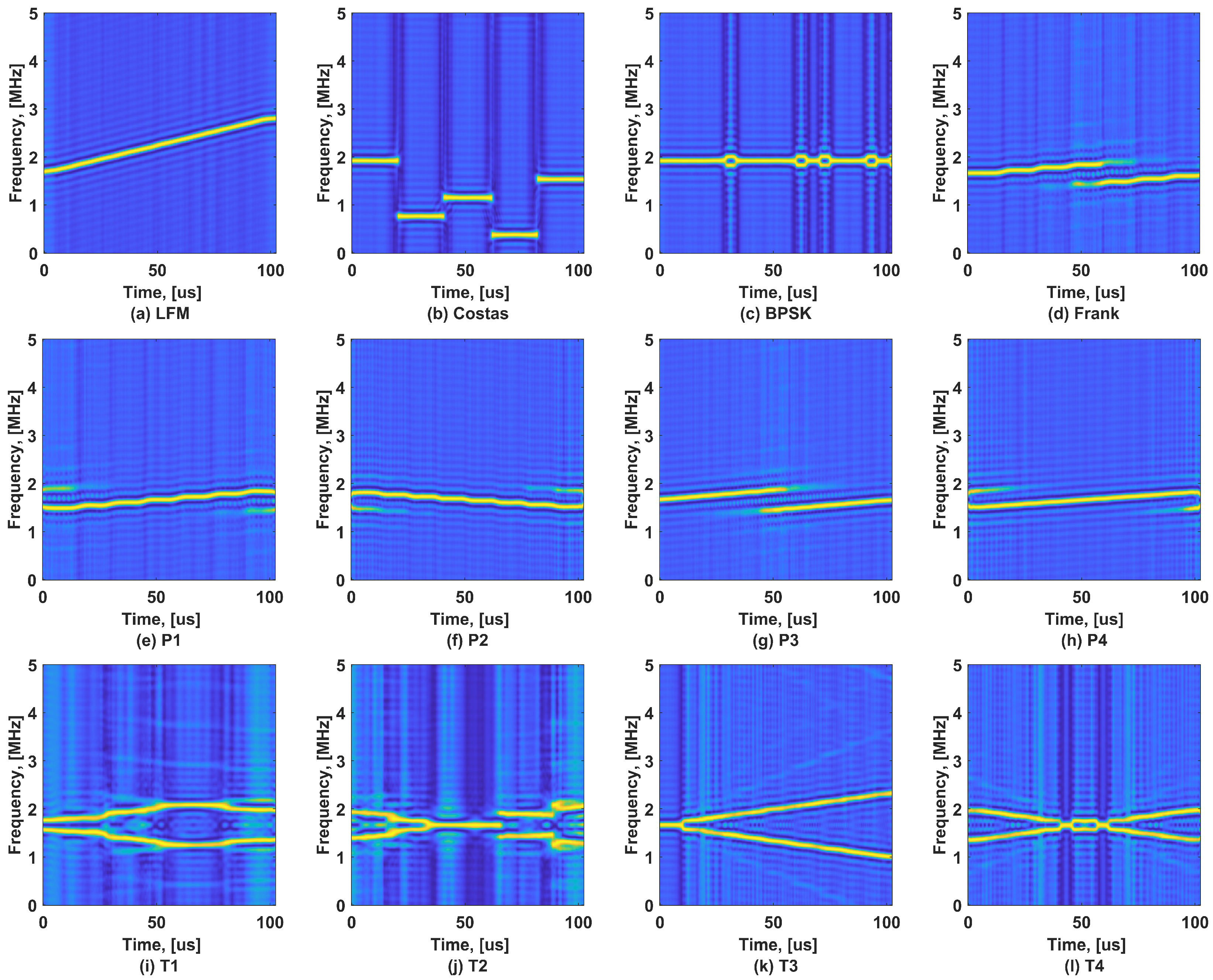
where f is the frequency variable, τ is the time delay, u is the time variable, and σ is the attenuation factor. The σ is a positive value, which is proportional to the amplitude of the cross term. The value of σ is larger, and the resolution of CWD TFIs is better, but it also results in a more pronounced cross term. Figure 2 shows the TFIs of twelve LPI radar signal waveforms. All signals are generated under the conditions of an SNR of 10 dB with a sampling rate of 100 MHz. It can be seen that different signal time–frequency images exhibit different time–frequency distribution characteristics.

2.2. Feature Enhancement Network

To fully extract the fine-grained features in TFIs for signal recognition, we propose a feature enhancement network with attention-based dynamic feature extraction blocks. Meanwhile, we introduce deep metric learning to further reduce noise interference and enhance the time–frequency features. Previous studies [33] typically used traditional image processing techniques such as cropping, binarization, and filtering to minimize noise interference in signal detection. However, while these approaches may be effective for suppressing noise, they can also inadvertently remove valuable characteristics, leading to information loss. To solve this issue, we propose an encoder–decoder structured feature enhancement network that suppresses noise while enhancing time–frequency characteristics.
The proposed feature enhancement network consists of three pairs of encoder–decoder blocks and several attention-based dynamic feature extraction blocks, as illustrated in the middle of Figure 2, incorporating skip links to facilitate information flow and feature reuse. To acquire low-dimensional feature representations, the three encoders perform 4× downsampling. These representations are subsequently input to the dynamic feature extraction blocks for further learning. Finally, an operation involving 2D convolutions and a corresponding 4× upsampling is applied to generate the enhanced TFIs. The main parameters of the feature enhancement network are detailed in Table 1.

2.2.1. Attention-Based Dynamic Feature Extraction Block

To address the challenge of extracting effective features from TFIs under low SNR conditions, this paper proposes an attention-based dynamic feature extraction (ADFE) block. This module is used to adaptively extract effective features from TFIs under low SNR conditions, as shown in Figure 3A. The ADFE block specifically consists of four convolutional layers, one feature attention block, and one deformable convolutional layer. Local residual learning is introduced at different network layers. Local residual learning can learn high-level features more efficiently by extracting and exploiting diverse features from multiple levels. Furthermore, with the addition of residual connections, the network can better capture feature dependencies, skipping less relevant information such as noise or low-frequency regions.
In the ADFE block, we present a feature attention block, which comprises a channel attention layer and a spatial attention layer. It can aid the model in simultaneously taking into account information from various regions and channels of the image, thereby enhancing its ability to capture the image features and their relationships more effectively. Figure 3C depicts the structure of the spatial attention layer. To calculate the weights at different pixel locations, the input features are processed by two convolutional layers with a 1 × 1 kernel size. This process ultimately assigns varying weights to different pixel positions in the input features, thus enhancing the response in critical regions. The operation of the spatial attention layer can be formulated as follows:
F s = F γ ( f 1 × 1 ( σ ( f 1 × 1 ( F ) ) ) )
where F represents the input features, f 1 × 1 represents the convolutional layer with a 1 × 1 kernel size, σ is the ReLU activation function, and γ is the sigmoid activation function.
Unlike the spatial attention layer, the channel attention layer (as depicted in Figure 3B) captures the overall feature of each channel using global average pooling. Subsequently, it calculates and assigns weights to individual channels. The channel attention layer can be represented as follows:
F c = F γ ( f 1 × 1 ( σ ( f 1 × 1 ( A v g p o o l ( F ) ) ) ) )
where Avgpool represents the global average pooling.
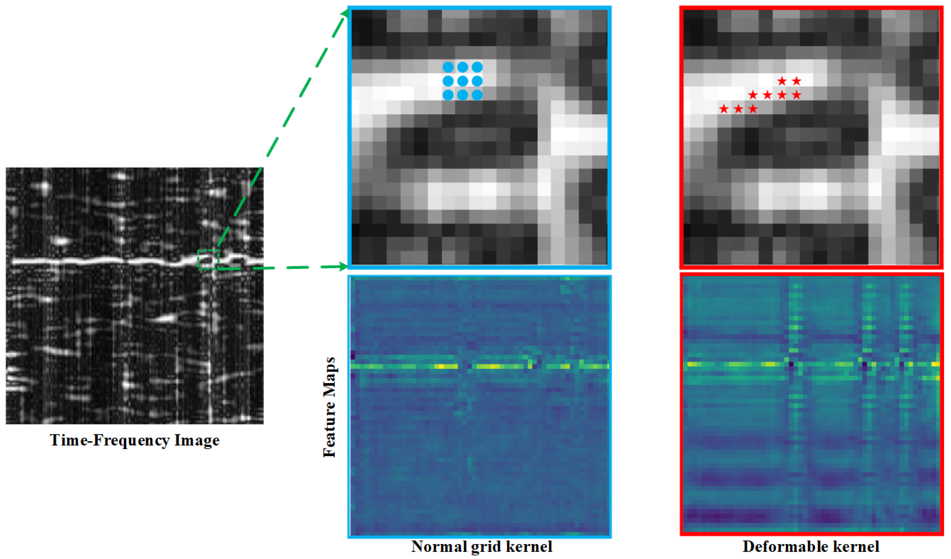
Following the feature attention block, we introduce a deformable convolution layer to capture vital information by employing a dynamic and adaptable variable convolution kernel. Different from grid convolution kernels with spatially fixed features (as illustrated in the center of Figure 4), the deformable convolution layer extends the receptive field through accommodating adaptive shape changes, as demonstrated on the right side of Figure 4. Therefore, by prioritizing the extraction of effective features from TFIs in the presence of noise interference, the model’s performance can be improved. Detailed parameters for the ADFE block are presented in Table 2.

2.2.2. Metric Learning with Triplet Loss

In order to enhance the discriminability of the fine-grained features learned by the ADFE blocks for various types of radar signals, we take additional steps to refine the TFI feature representations under low SNR conditions. This is achieved by introducing deep metric learning during the training phase within the feature space. Existing LPI radar signal recognition methods based on deep learning generally utilize deep neural network architectures to extract features from TFIs [34,35,36]. However, under low SNR conditions, deep neural networks often face challenges in extracting discriminate features for various signals. Some recent work that combines deep learning with metric learning has gained much attention [37,38,39]. Deep metric learning involves training a model using a metric loss function that encourages the model to map similar samples close together in feature space and distant from dissimilar samples [40]. Furthermore, deep metric learning can leverage the utilization of extensive labeled data, enabling the model to learn robust and distinctive distance measures [41].
In this paper, we incorporate a triplet loss to further enhance the representation of TFI features in low SNR conditions with the feature space. Typically, the triplet loss is defined by using three samples: positive, negative, and anchor. It aims to encourage the distance between the anchor and the positive sample to be smaller than the distance between the anchor and the negative sample by a certain margin. In the feature enhancement network, we represent the enhanced TFI ( ϕ ) as the anchor sample, the clean and noise-free TFI (J) as the positive sample, and the TFI obtained from the receiver (I) as the negative sample. During the training phase, we utilize triplet loss to impose constraints that minimize the distance between ϕ and J while simultaneously maximizing the distance between ϕ and I. We can enhance the ability of the feature enhancement network to express TFI features in low SNR conditions. We use the pre-trained VGG-11 model, where fully connected layers (G) are removed to obtain shared features. The VGG-11 model is pre-trained on ImageNet. Pre-trained weights provide a strong initialization to the feature extractor, allowing it to extract meaningful features immediately instead of learning them from scratch. The objective function of the triplet loss can be represented as [42]:
L triplet = max i m G ( ϕ ( I ) ) i a G ( J ) i p 2 2 G ( ϕ ( I ) ) i a G ( I ) i n 2 2 + margin , 0
where G ( ) i a is the feature of anchor sample, G ( ) i p is the feature of positive sample, and G ( ) i n is the feature of negative sample.
Moreover, we use L1-loss as the reconstruction loss to directly measure the pixel-level difference between I and J. The L1-loss can make the output of the feature enhancement network closer to J. The expression of L1-loss is:
L l 1 = min J ϕ ( I ) 1
Finally, we incorporate the triplet loss and L1-loss into the metric learning framework for model training. The overall objective function of the feature enhancement network is formulated as:
L * = L l 1 + λ L triplet
where λ is the weight factor. In experiments, we use the grid search parameter method to search the value of λ to obtain the best recognition performance. When λ = 0.12 , better results can be obtained. During model training, the triplet loss further provides additional constraints on the extracted features within the feature space, effectively mitigating the issue of L1-loss sensitivity to outliers. By this metric learning process, we obtain discriminative and stable TFI features, which help to improve the recognition performance for subsequent classification networks.

2.3. Classification Network

To achieve efficient recognition of a variety of LPI radar signals, we develop a straightforward and efficient classification network based on the feature representations learned through the feature enhancement network, depicted on the right side of Figure 1. The classification network consists of two fully connected layers with different sizes. The first fully connected layer is used to transform high-dimensional image features into low-dimensional ones. On one hand, it reduces the subsequent computational cost. On the other hand, during training, we enforce a margin between the same category by using the center loss function. This method allows for tighter integration of TFI features of LPI radar signals of the same modulation types. The formulation of the center loss ( L c ) function is:
L c = 1 2 i = 1 m x i c y i 2 2
where x i is the ith feature after the full connection layers and c y i denotes the feature center of y i th class.
The second fully connected layer can be used to map the features to the dimensions matching the number of LPI radar signals. Actually, we have utilized the softmax loss ( L s ), which is the most widely used in the recognition task to complete the recognition of the final LPI radar signal, and its expression is [43]:
L s = i = 1 m log e W y i T x i + b y i j = 1 n e W j T x i + b j
where x i is the ith input feature defined by the label y i ( i ( 1 , m ) , m is the number of classes), b is the bias parameter, and W j is the weight parameter of the jth column in the fully connected layer (j is the number of min-batch size).
Finally, we merge the aforementioned two loss functions in order to optimize the closeness of intra-class distances and the discernibility of inter-class distances, ensuring that TFI features are both distinguishable and stable. The joint loss formula is as follows:
L = L s + β L c
where L s is the SoftMax loss function and β is the weight factor.

3. Experiments

3.1. Experimental Settings and Baselines

To evaluate the recognition performance of the proposed signal identification approach, we use twelve typical LPI radar signals in our experiments. The specific signal parameters and their descriptions are shown in Table 3. We generate 200 samples for each signal type under each SNR and form a training set, where the SNR ranges from −14 dB to 10 dB with a step size of 2 dB, and the total number of training set samples is 31,200. In addition, we generate 80 samples for each type of signal to form a validation set, where the SNR ranges from −16 dB to 10 dB, with a step size of 2 dB, and the total number of validation set samples is 13,440. All experiments are implemented on a computer with an AMD EPYC 7F52 16-core @ 3.90 GHz CPU, an NVIDIA GeForce RTX3090 GPU, and an operating system of Ubuntu 18.04 server version.
Furthermore, we compare the proposed method to various advanced techniques. The baselines include LPI-net [27], which achieves accurate recognition of radar signals with multiple cascaded CNN modules, CDAE-DCNN [28], which achieves LPI radar signal recognition at low SNR conditions by de-noising the TFIs, and LDC-Unet [29], which passes through a locally densely connected network to extract and enhance the TFI features to achieve the recognition task. All algorithms were executed 10 times, and the reported results represent the average performance.

3.2. Performance Comparison

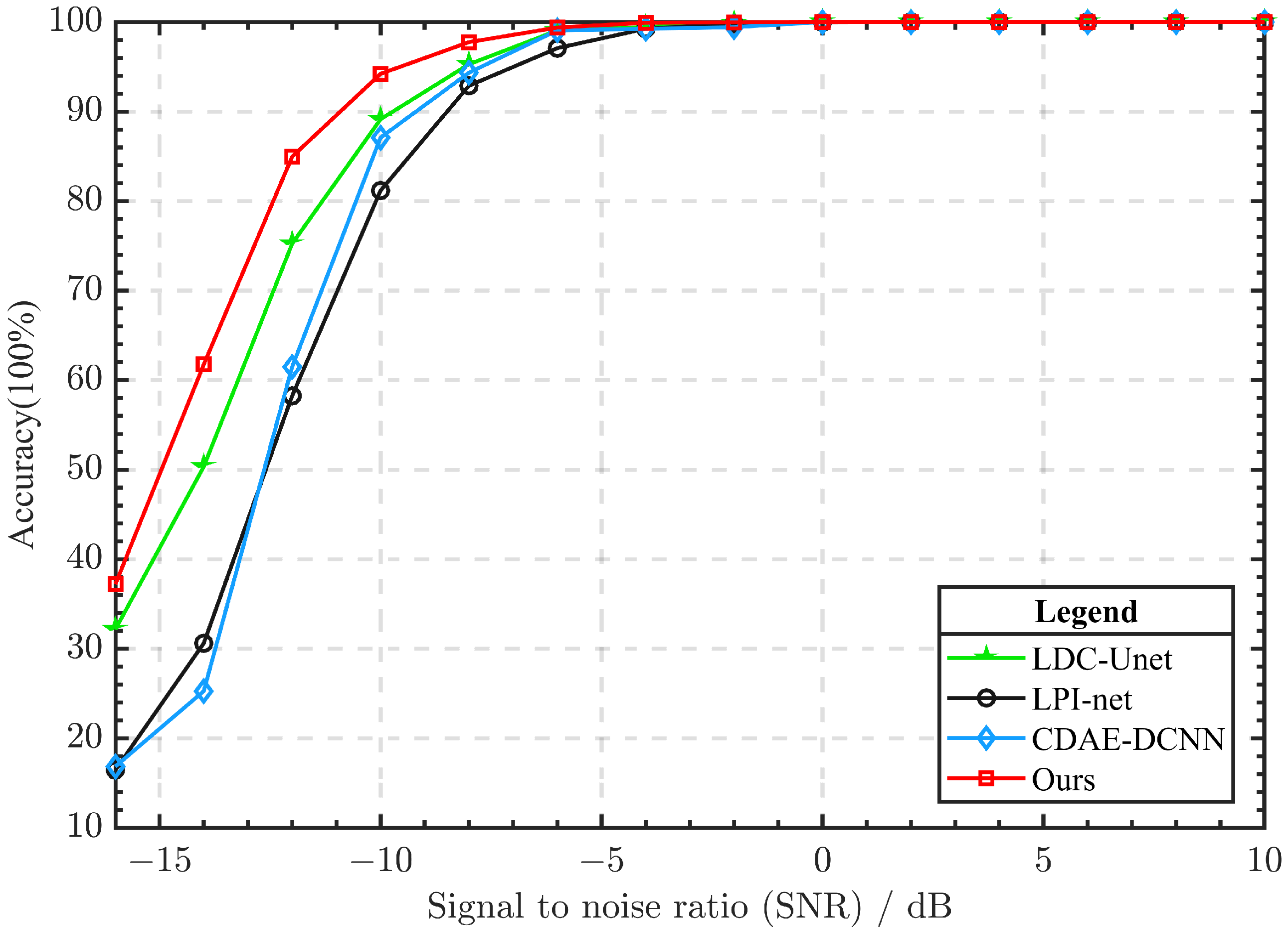
In this section, we evaluate the recognition performance of the proposed method in comparison to LDC-Unet, LPI-Net, and CDAE-DCNN. Figure 5 illustrates the recognition accuracy of different methods under different SNR conditions. It can be seen that the recognition performance of all methods declines as the SNR decreases. However, the proposed method achieves higher recognition accuracy than the other three advanced methods. When the SNR ≤ −6 dB, the recognition performance of LPI-Net and CDAE-DCNN severely decreases, mainly because their simple network structures make it challenging to extract effective features under low SNR conditions. The proposed method, as well as LDC-Unet, enhances feature extraction by adding additional network modules. Even when SNR = −10 dB, the recognition accuracy of the two methods still exceeds 90%. Furthermore, the proposed method obtains a higher recognition accuracy compared to LDC-Unet when SNR is less than −5 dB.
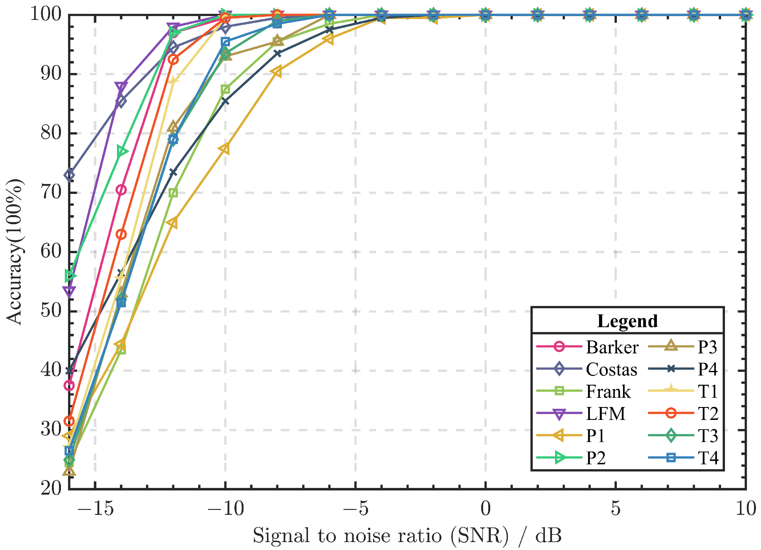
In order to further reveal the recognition accuracy of the method proposed for different modulation types of radar signals, we examine the recognition accuracy of twelve different modulation types of LPI radar signals under various SNR conditions, as shown in Figure 6. For SNR = −10 dB, the recognition accuracy of LFM, Costas, T1 code, and T2 code remains above 95%. The above signals still maintain a high recognition accuracy as the SNR decreases. In comparison, at SNR = −10 dB, the recognition accuracy of P1, P4, and Frank is less than 90% and shows a serious downward trend as the SNR decreases. It is worthy of noting that the identification accuracy of LPI radar signals based on the polyphase modulation type is significantly lower compared with other modulation types. This difference is mainly attributed to the low immunity of polyphase modulation to noise.

3.3. Computational Cost

In this section, we utilize three metrics, namely FLOPs (floating point operations), network parameters, and inference time, to assess the computational cost of the proposed method. Table 4 shows the computational costs of the proposed method and three other methods. The inference time is calculated on the CPU under the same hardware conditions. From the table, it can be concluded that the computational cost of LPI-Net and CDAE-DCNN is lower than that of LDC-Unet and the proposed method. This is mainly because the structure of their feature extraction components is simple. Therefore, this also leads to the difficulty of achieving satisfactory recognition performance for both the LPI-Net and CDAE-DCNN in low SNR conditions. The proposed method has a lower computational cost compared to LDC-Unet, mainly due to the use of parameter reuse technology. Parameter reuse technology refers to reusing calculated parameters during model training to reduce the amount of calculation and improve training speed. In the manuscript, our multiple ADFE blocks are calculated with the same parameters, reducing the number of parameters.

3.4. Ablation Experiment

3.4.1. Effect of Feature Enhancement Network

To evaluate the effect of the proposed feature enhancement network on recognition performance under low SNR conditions, we define a variant of the proposed method, which removes the feature enhancement network. As shown in Figure 7, when the SNR is less than −4 dB, the recognition performance of the variant without using the feature enhancement network rapidly declines. The main reason for this phenomenon is that it is difficult to extract effective TFI features with a simple feature extraction structure under low SNR conditions. In contrast, our proposed method achieves an overall recognition accuracy of over 94% in the range of −10 dB to −4 dB for SNR. This ablation experiment suggests that the feature enhancement network greatly improves the recognition performance under low SNR conditions.
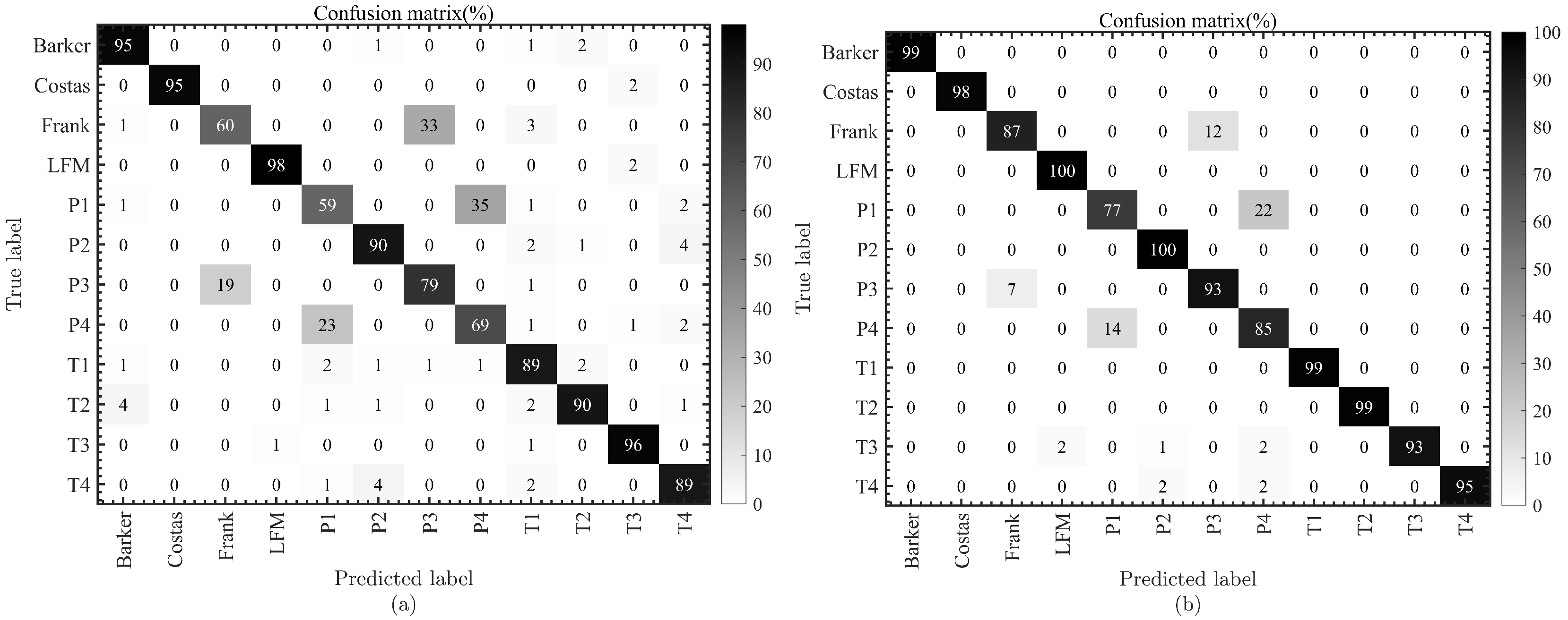
We employ a confusion matrix to analyze the reasons for the mutual influence between different modulation types of LPI radar signals under low SNR conditions, as shown in Figure 8. Figure 8a shows the confusion matrix of the variant without the feature enhancement network at SNR = −10 dB. Obviously, LPI radar signals with similar time–frequency features are prone to confusion with each other, such as P1, P3, P4, and Frank codes. For the P1 code, 35% is misidentified as the P4 code, and for the P4 code, 23% is misidentified as the P1 code. In addition, 33% of Frank codes are identified as P3 codes. The reason is that under low SNR conditions, the effective features are blurred, reducing the recognition accuracy. On the contrary, the proposed method addresses the challenge of feature extraction under low SNR conditions by utilizing the feature enhancement network, as shown in Figure 8b. This reduces the likelihood of mutual confusion between different signals.

3.4.2. Effect of ADFE Blocks

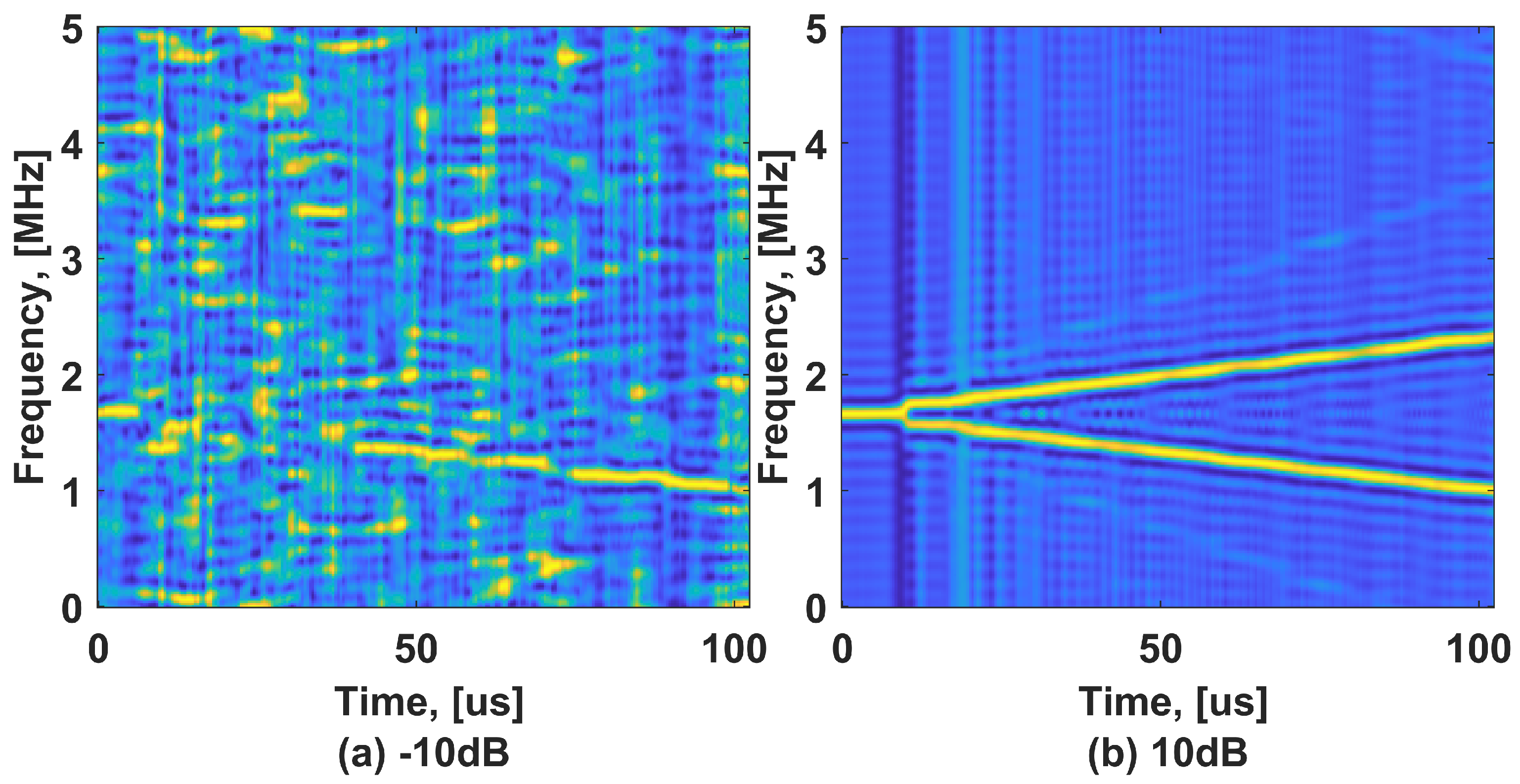
To assess the impact of the proposed ADFE blocks on recognition performance in low SNR conditions, Figure 9 illustrates the recognition accuracy at various SNRs for different numbers of ADFE blocks. For SNR ≤ −5 dB, the recognition performance of the feature enhancement network without the ADFE block sharply declines. The main reason is that under low SNR conditions, the TFI features are missing or blurry, and simple encoders and decoders cannot extract effective features, as shown in Figure 10. However, by incorporating the ADFE block with deformable convolution and an attention mechanism, the feature enhancement network’s capability of extracting effective features under low SNR conditions is greatly improved.
With the increase in the number of ADFE blocks, we observed an overall improvement in recognition performance. However, after increasing the number of ADFE blocks to a certain level, the overall recognition performance starts to decline. The experiment shows that when the number of ADFE blocks increases to eight, the overall recognition performance is comparable to using four ADFE blocks. In fact, Ref. [44] has proven that the performance of a neural network architecture does not necessarily improve with increased depth. On the one hand, training becomes challenging due to optimization costs. On the other hand, the ADFE module designed in this paper uses parameter sharing to reduce parameter storage costs, which limits the diversity of feature representation to some extent. In order to balance the performance and the computational costs, we utilize six ADFE blocks in the feature enhancement network to improve the capability of feature extraction under low SNR conditions.

3.4.3. Effect of Metric Learning

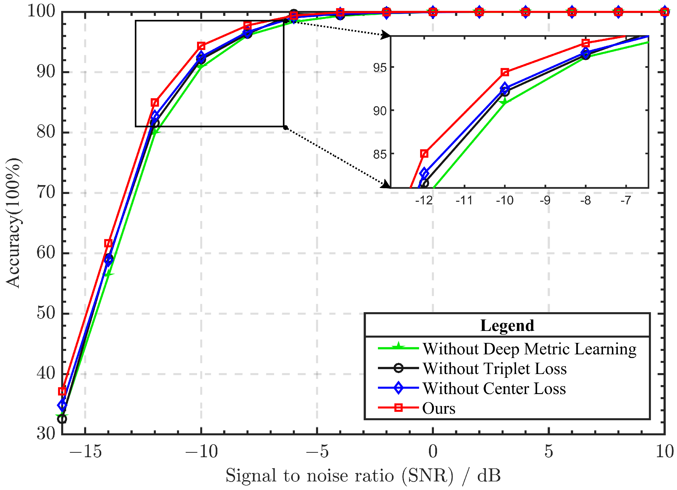
To assess the influence of deep metric learning on recognition performance, we individually removed the center loss and triplet loss components employed in the proposed methods, as depicted in Figure 11. It can be seen that for SNR ≤ −5 dB, the incorporation of deep metric learning in the proposed methods enhances the recognition accuracy by around 5% compared to when it is not used. This suggests that introducing metric learning to optimize the distance between samples in the feature space effectively improves the recognition accuracy of the proposed methods under low SNR conditions. Moreover, when compared to triplet loss, center loss achieves a slightly higher recognition accuracy by directly optimizing the compactness of intra-class features.

3.5. Robustness Experiment

The above experiment demonstrates that the proposed method has excellent recognition performance. However, in practical situations, the parameters of the signals intercepted by the receiver may deviate from the training dataset used in our experiments. In order to study the robustness of the proposed method, we test the method on a new dataset with different parameters from the training set. Table 5 shows the parameter settings used for the new dataset. As shown in Figure 12, when the test parameters are different from the training parameters, the recognition performance also decreases slightly but still maintains a high recognition accuracy when SNR ≥ 0 dB. However, the recognition accuracy of the proposed method has significantly decreased as SNR decreases. When SNR ≤ −5 dB, due to overfitting during the training process, the overall recognition accuracy is less than 80%, much lower than the results without parameter deviation. Therefore, how to more effectively improve the robustness of the model is the focus of our future research.

4. Conclusions

In this paper, we propose a novel radar signal recognition method to solve the problem of low recognition accuracy under low SNR conditions by introducing a feature enhancement network with deep metric learning. To achieve this goal, we have developed a pre-training feature enhancement network that enhances TFI features in the presence of noise interference. In the feature enhancement network, we have designed an ADFE block that can adaptively extract TFI features under low SNR conditions. Furthermore, we have incorporated deep metric learning into the feature enhancement network to guarantee the distinguishability and stability of the extracted TFI features. We have verified, through ablation experiments, that the ADFE block and deep metric learning contribute to improving recognition performance. Finally, the experimental results show that compared with three advanced LPI radar signal recognition methods, LPI-net, CDAE-DCNN, and LDC-Unet, the proposed method achieves better recognition performance under low SNR conditions.

Author Contributions

Conceptualization, D.Q.; methodology, F.R.; software, F.R.; validation, L.S.; formal analysis, X.W.; investigation, D.Q.; resources, H.L.; data curation, L.S.; writing—original draft preparation, F.R.; writing—review and editing, X.W.; visualization, X.W.; supervision, D.Q.; project administration, H.L.; funding acquisition, D.Z. All authors have read and agreed to the published version of the manuscript.

Funding

This research was supported by Key Research and Development Projects in Zhejiang Province (No. 2022C01144).

Data Availability Statement

Data are contained within the article.

Acknowledgments

The authors wish to express their appreciation to the editors for their rigorous and efficient work and the reviewers for their helpful suggestions, which greatly improved the presentation of this paper.

Conflicts of Interest

The authors declare that they have no conflict of interest to report regarding the present study. Author H.L. is an employee of Jptek Corporation Limited Hangzhou. The paper reflects the views of the scientist, and not the company.

References

  1. Schleher, D. LPI radar: Fact or fiction. IEEE Aerosp. Electron. Syst. Mag. 2006, 21, 3–6. [Google Scholar] [CrossRef]
  2. Galati, G.; Pavan, G.; Wasserzier, C. Signal design and processing for noise radar. EURASIP J. Adv. Signal Process. 2022, 2022, 52. [Google Scholar] [CrossRef]
  3. Galati, G.; Pavan, G. Noise Radar Technology and Quantum Radar: Yesterday, Today and Tomorrow. In Proceedings of the 2022 IEEE 2nd Ukrainian Microwave Week (UkrMW), Kharkiv, Ukraine, 14–18 November 2022; pp. 504–511. [Google Scholar]
  4. Dunde, V.; Nallapati, S.; Thakkallapally, S.R.; Chetla, B.P.; Kethireddy, S.P. Design and Analysis of LPI Radar Waveforms. In Proceedings of the 2022 International Conference on Recent Trends in Microelectronics, Automation, Computing and Communications Systems (ICMACC), Hyderabad, India, 28–30 December 2022; pp. 1–6. [Google Scholar]
  5. Savci, K.; Stove, A.G.; De Palo, F.; Erdogan, A.Y.; Galati, G.; Lukin, K.A.; Lukin, S.; Marques, P.; Pavan, G.; Wasserzier, C. Noise radar—Overview and recent developments. IEEE Aerosp. Electron. Syst. Mag. 2020, 35, 8–20. [Google Scholar] [CrossRef]
  6. Jia, J.; Han, Z.; Liu, L. Review on Low Intercept Radar Signal Design Technology. In Proceedings of the 2022 IEEE 4th International Conference on Power, Intelligent Computing and Systems (ICPICS), Shenyang, China, 29–31 July 2022; pp. 434–437. [Google Scholar]
  7. Ou, J.; Zhang, J.; Zhan, R. Processing technology based on radar signal design and classification. Int. J. Aerosp. Eng. 2020, 2020, 4673763. [Google Scholar] [CrossRef]
  8. Meng, F.; Chen, P.; Wu, L.; Wang, X. Automatic modulation classification: A deep learning enabled approach. IEEE Trans. Veh. Technol. 2018, 67, 10760–10772. [Google Scholar] [CrossRef]
  9. Wang, S.Q.; Zhou, G.A.; Song, B.J.; Gao, C.Y.; Wan, P.F. Research on radar emitter signal feature extraction method based on fuzzy entropy. Procedia Comput. Sci. 2019, 154, 508–513. [Google Scholar] [CrossRef]
  10. Mingqiu, R.; Jinyan, C.; Yuanqing, Z.; Jun, H. Radar signal feature extraction based on wavelet ridge and high order spectral analysis. In Proceedings of the 2009 IET International Radar Conference, Guilin, China, 20–22 April 2009. [Google Scholar]
  11. Travassos, X.L.; Avila, S.L.; Ida, N. Artificial neural networks and machine learning techniques applied to ground penetrating radar: A review. Appl. Comput. Inform. 2020, 17, 296–308. [Google Scholar] [CrossRef]
  12. Kotsiantis, S.B. Decision trees: A recent overview. Artif. Intell. Rev. 2013, 39, 261–283. [Google Scholar] [CrossRef]
  13. Bansal, M.; Goyal, A.; Choudhary, A. A comparative analysis of K-nearest neighbor, genetic, support vector machine, decision tree, and long short term memory algorithms in machine learning. Decis. Anal. J. 2022, 3, 100071. [Google Scholar] [CrossRef]
  14. Cervantes, J.; Garcia-Lamont, F.; Rodríguez-Mazahua, L.; Lopez, A. A comprehensive survey on support vector machine classification: Applications, challenges and trends. Neurocomputing 2020, 408, 189–215. [Google Scholar] [CrossRef]
  15. Pisner, D.A.; Schnyer, D.M. Support vector machine. In Machine Learning; Elsevier: Amsterdam, The Netherlands, 2020; pp. 101–121. [Google Scholar]
  16. Zhu, J.; Zhao, Y.; Tang, J. Automatic recognition of radar signals based on time-frequency image character. In Proceedings of the 2013 IET International Radar Conference, Xi’an, China, 14–16 April 2013; pp. 1–6. [Google Scholar]
  17. Zhang, Z.; Li, Y.; Jin, S.; Zhang, Z.; Wang, H.; Qi, L.; Zhou, R. Modulation signal recognition based on information entropy and ensemble learning. Entropy 2018, 20, 198. [Google Scholar] [CrossRef] [PubMed]
  18. Huang, Y.; Jin, W.; Li, B.; Ge, P.; Wu, Y. Automatic modulation recognition of radar signals based on manhattan distance-based features. IEEE Access 2019, 7, 41193–41204. [Google Scholar] [CrossRef]
  19. Abdelmutalab, A.; Assaleh, K.; El-Tarhuni, M. Automatic modulation classification based on high order cumulants and hierarchical polynomial classifiers. Phys. Commun. 2016, 21, 10–18. [Google Scholar] [CrossRef]
  20. Li, L.; Dong, Z.; Zhu, Z.; Jiang, Q. Deep-learning hopping capture model for automatic modulation classification of wireless communication signals. IEEE Trans. Aerosp. Electron. Syst. 2022, 59, 772–783. [Google Scholar] [CrossRef]
  21. Li, L.; Zhu, Y.; Zhu, Z. Automatic Modulation Classification Using ResNeXt-GRU with Deep Feature Fusion. IEEE Trans. Instrum. Meas. 2023, 72, 2519710. [Google Scholar] [CrossRef]
  22. Xiao, W.; Luo, Z.; Hu, Q. A Review of Research on Signal Modulation Recognition Based on Deep Learning. Electronics 2022, 11, 2764. [Google Scholar] [CrossRef]
  23. Ren, B.; Teh, K.C.; An, H.; Gunawan, E. Automatic Modulation Recognition of Dual-Component Radar Signals Using ResSwinT-SwinT Network. IEEE Trans. Aerosp. Electron. Syst. 2023, 59, 6405–6418. [Google Scholar] [CrossRef]
  24. Zhang, M.; Diao, M.; Guo, L. Convolutional Neural Networks for Automatic Cognitive Radio Waveform Recognition. IEEE Access 2017, 5, 11074–11082. [Google Scholar] [CrossRef]
  25. Wan, J.; Yu, X.; Guo, Q. LPI radar waveform recognition based on CNN and TPOT. Symmetry 2019, 11, 725. [Google Scholar] [CrossRef]
  26. Kong, S.H.; Kim, M.; Hoang, L.M.; Kim, E. Automatic LPI radar waveform recognition using CNN. IEEE Access 2018, 6, 4207–4219. [Google Scholar] [CrossRef]
  27. Huynh-The, T.; Doan, V.S.; Hua, C.H.; Pham, Q.V.; Nguyen, T.V.; Kim, D.S. Accurate LPI Radar Waveform Recognition with CWD-TFA for Deep Convolutional Network. IEEE Wirel. Commun. Lett. 2021, 10, 1638–1642. [Google Scholar] [CrossRef]
  28. Qu, Z.; Wang, W.; Hou, C.; Hou, C. Radar signal intra-pulse modulation recognition based on convolutional denoising autoencoder and deep convolutional neural network. IEEE Access 2019, 7, 112339–112347. [Google Scholar] [CrossRef]
  29. Jiang, W.; Li, Y.; Liao, M.; Wang, S. An improved LPI radar waveform recognition framework with LDC-Unet and SSR-Loss. IEEE Signal Process. Lett. 2021, 29, 149–153. [Google Scholar] [CrossRef]
  30. Wu, H.; Qu, Y.; Lin, S.; Zhou, J.; Qiao, R.; Zhang, Z.; Xie, Y.; Ma, L. Contrastive learning for compact single image dehazing. In Proceedings of the IEEE/CVF Conference on Computer Vision and Pattern Recognition, Nashville, TN, USA, 20–25 June 2021; pp. 10551–10560. [Google Scholar]
  31. Ghadimi, G.; Norouzi, Y.; Bayderkhani, R.; Nayebi, M.; Karbasi, S. Deep learning-based approach for low probability of intercept radar signal detection and classification. J. Commun. Technol. Electron. 2020, 65, 1179–1191. [Google Scholar] [CrossRef]
  32. Choi, H.I.; Williams, W.J. Improved time-frequency representation of multicomponent signals using exponential kernels. IEEE Trans. Acoust. Speech Signal Process. 1989, 37, 862–871. [Google Scholar] [CrossRef]
  33. Si, W.; Wan, C.; Deng, Z. Intra-pulse modulation recognition of dual-component radar signals based on deep convolutional neural network. IEEE Commun. Lett. 2021, 25, 3305–3309. [Google Scholar] [CrossRef]
  34. Dai, G.; Xie, J.; Fang, Y. Deep correlated holistic metric learning for sketch-based 3D shape retrieval. IEEE Trans. Image Process. 2018, 27, 3374–3386. [Google Scholar] [CrossRef]
  35. Li, Z.; Tang, J. Weakly supervised deep metric learning for community-contributed image retrieval. IEEE Trans. Multimed. 2015, 17, 1989–1999. [Google Scholar] [CrossRef]
  36. Harwood, B.; Kumar BG, V.; Carneiro, G.; Reid, I.; Drummond, T. Smart mining for deep metric learning. In Proceedings of the IEEE International Conference on Computer Vision, Venice, Italy, 22–29 October 2017; pp. 2821–2829. [Google Scholar]
  37. Martin-Donas, J.M.; Gomez, A.M.; Gonzalez, J.A.; Peinado, A.M. A deep learning loss function based on the perceptual evaluation of the speech quality. IEEE Signal Process. Lett. 2018, 25, 1680–1684. [Google Scholar] [CrossRef]
  38. Elezi, I.; Vascon, S.; Torcinovich, A.; Pelillo, M.; Leal-Taixé, L. The group loss for deep metric learning. In Proceedings of the 16th European Conference on Computer Vision (ECCV 2020), Glasgow, UK, 23–28 August 2020; Proceedings Part VII 16. pp. 277–294. [Google Scholar]
  39. Jiang, W.; Huang, K.; Geng, J.; Deng, X. Multi-scale metric learning for few-shot learning. IEEE Trans. Circuits Syst. Video Technol. 2020, 31, 1091–1102. [Google Scholar] [CrossRef]
  40. Zhe, X.; Chen, S.; Yan, H. Directional statistics-based deep metric learning for image classification and retrieval. Pattern Recognit. 2019, 93, 113–123. [Google Scholar] [CrossRef]
  41. Mohan, D.D.; Sankaran, N.; Fedorishin, D.; Setlur, S.; Govindaraju, V. Moving in the right direction: A regularization for deep metric learning. In Proceedings of the IEEE/CVF Conference on Computer Vision and Pattern Recognition, Seattle, WA, USA, 13–19 June 2020; pp. 14591–14599. [Google Scholar]
  42. Schroff, F.; Kalenichenko, D.; Philbin, J. Facenet: A unified embedding for face recognition and clustering. In Proceedings of the IEEE Conference on Computer Vision and Pattern Recognition, Boston, MA, USA, 7–12 June 2015; pp. 815–823. [Google Scholar]
  43. De Boer, P.T.; Kroese, D.P.; Mannor, S.; Rubinstein, R.Y. A tutorial on the cross-entropy method. Ann. Oper. Res. 2005, 134, 19–67. [Google Scholar] [CrossRef]
  44. He, K.; Zhang, X.; Ren, S.; Sun, J. Deep residual learning for image recognition. In Proceedings of the IEEE Conference on Computer Vision and Pattern Recognition, Las Vegas, NV, USA, 27–30 June 2016; pp. 770–778. [Google Scholar]
Figure 1. The overall architecture of the proposed method.
Electronics 12 04934 g001
Figure 2. The CWD transformation images of twelve kinds of LPI radar signals.
Electronics 12 04934 g002
Figure 3. The proposed ADFE block structure. (A) The overall structure of the ADFE block. (B) Channel attention structure. (C) Spatial attention structure.
Electronics 12 04934 g003
Figure 4. Comparison of the sampling locations of standard CNN and deformable CNN. The dots represent the structure of the standard convolution kernel. The stars represent the structure of the deformable convolution kernel.
Electronics 12 04934 g004
Figure 5. Effect of feature enhancement network and center loss on classification performance.
Electronics 12 04934 g005
Figure 6. Visualization of feature distribution.
Electronics 12 04934 g006
Figure 7. Effect of feature enhancement network on recognition performance.
Electronics 12 04934 g007
Figure 8. The confusion matrix for (a) the variant without feature enhancement network; (b) our proposed method.
Electronics 12 04934 g008
Figure 9. Effect of ADFE blocks on recognition performance.
Electronics 12 04934 g009
Figure 10. T3 time–frequency image at (a) −10 dB SNR; (b) 10 dB SNR.
Electronics 12 04934 g010
Figure 11. Effect of deep metric learning on recognition performance.
Electronics 12 04934 g011
Figure 12. Effect of parameter deviation on recognition performance.
Electronics 12 04934 g012
Table 1. Detailed parameters of feature enhancement network.
Layer NameTypeOutput SizeChannelStrideKernel Size
Encoder #1Conv2d
Relu
256 × 256 × 646417 × 7
Encoder #2Conv2d
Relu
128 × 128 × 1281282 × 23 × 3
Encoder #3Conv2d
Relu
64 × 64 × 2562562 × 23 × 3
ADFE Block #1–#6-64 × 64 × 256256--
Decoder #1ConvTranspose2d
Relu
128 × 128 × 1281282 × 23 × 3
Decoder #2ConvTranspose2d
Relu
256 × 256 × 64642 × 23 × 3
Decoder #3Conv2d
Tanh
256 × 256 × 1117 × 7
Table 2. Detailed parameters of ADFE block.
Layer NameTypeFilterSize
Conv2D #1–#2Conv2D643 × 3
Relu--
Channel Attention #3Avgpool--
Conv2D81 × 1
Relu--
Conv2D641 × 1
Sigmod--
Spatial Attention #4Conv2D81 × 1
Relu--
Conv2D641 × 1
Sigmod--
Conv2D #5Conv2D643 × 3
DCN Block #6deformable convolution643 × 3
Conv2D #7Conv2D643 × 3
Table 3. LPI waveform parameters.
Radar WaveformSimulation ParameterRanges
Sampling frequency f s 100 MHz
LFMInitial frequency f 0 U ( 1 / 6 , 1 / 5 ) 1 f s
Bandwidth B U ( 1 / 20 , 1 / 16 ) f s
BPSKCode length N c {7,11,13}
Center frequency f c U ( 1 / 6 , 1 / 5 ) f s
CostasFundamental frequency U ( 1 / 30 , 1 / 24 ) f s
Hopping frequency f h {3,4,5,6} 2
Frank and P1–P4Carrier frequency f c U ( 1 / 6 , 1 / 5 ) f s
Cycles per phase code N c c {3,4,5}
T1–T4Number of segments k{4,5,6}
1  U ( ) means that the parameters are sampled from a continuous uniform distribution over a range. 2  { } means that the parameters are selected from a discrete set.
Table 4. Complexity of four methods.
MethodFLOPs [G] 1 Params [M] 2 Inference Time [ms]
LPI-Net1.4090.23283.172
CDAE-DCNN1.8030.768120.662
LDC-Unet21.3489.85273.405
This Paper18.8393.719160.188
1 [G] represents one billion floating-point operations per second. 2 [M] represents the unit of millions of parameters.
Table 5. Different parameter settings for the test set.
Radar SignalParameterTrain ParameterTest Parameter
LFMB U ( 1 / 6 , 1 / 5 ) f s U ( 1 / 16 , 1 / 8 ) f s
BPSK N c {7,11,13}{11,13}
Costas f h {3,4,5,6}{2,3,4,5}
Frank, P1–P4 N c c {3,4,5}{4,5,6}
T1–T4k{4,5,6}{3,4,5}
Disclaimer/Publisher’s Note: The statements, opinions and data contained in all publications are solely those of the individual author(s) and contributor(s) and not of MDPI and/or the editor(s). MDPI and/or the editor(s) disclaim responsibility for any injury to people or property resulting from any ideas, methods, instructions or products referred to in the content.