A Lightweight Multi-Scale Quadratic Separation Convolution Module for CNN Image-Classification Tasks

Abstract

Currently, most convolutional networks use standard convolution for feature extraction to pursue accuracy. However, there is potential room for improvement in terms of the number of network parameters and model speed. Therefore, this paper proposes a lightweight multi-scale quadratic separable convolution module (Mqscm). First, the module uses a multi-branch topology to maintain the sparsity of the network architecture. Second, channel separation and spatial separation methods are used to separate the convolution kernels, reduce information redundancy within the network, and improve the utilization of hardware computing resources. In the end, the module uses a variety of convolution kernels to obtain information on different scales to ensure the performance of the network. The performance comparison on three image-classification datasets shows that, compared with standard convolution, the Mqscm module reduces computational effort by approximately 44.5% and the model training speed improves by a range of 14.93% to 35.41%, maintaining performance levels comparable to those of deep convolution. In addition, compared with ResNet-50, the pure convolution network MqscmNet reduces the parameters by about 59.5%, saves the training time by about 29.7%, and improves the accuracy by 0.59%. Experimental results show that the Mqscm module reduces the memory burden of the model, improves efficiency, and has good performance.

1. Introduction

In the past decade, the field of computer vision has made groundbreaking progress and had a profound impact. The main driving factor is the rapid development of convolutional neural networks (CNNs) [1], which has made continuous breakthroughs in image classification [2], object detection [3], semantic segmentation [4], and other fields. Although the concept of the neuron was put forward as early as 1943, the new era of computer vision was not officially opened until 2012, when AlexNet [5] won the championship of ImageNet Vision Challenge [6,7]. Since then, new convolutional neural networks have appeared on the stage of the computer vision field almost every year. For example, VggNet [8], the Inception series [9,10,11], and the ResNet series [12,13,14].

The performance of convolutional neural networks is constantly breaking through, but at the moment, the performance improvements of most CNNs [15,16] are mainly achieved by deepening or broadening the network, resulting in increased computing and memory requirements [17]. To solve this problem, the field of convolutional neural networks has begun to focus on efficient network architecture, which can greatly reduce the computational pressure of the network while maintaining relatively good accuracy [18].

Now, most of the efficient CNNs mainly achieve performance improvements through engineering architectures, such as the structure of multiple convolution kernels, to obtain features of different scales for fusion [19], and the extracted feature information is better than the features extracted using a single convolution kernel and uses point convolution for dimensionality reduction and parameter reduction. ShuffleNet [20] uses channel shuffle operations to compensate for information exchange between groups. However, both of these structures increase the level of network fragmentation. Xception [21] uses depthwise separable convolution, which first separates channels, and then uses point convolution for channel interaction. Compared with standard convolution, the computational cost is sharply reduced, but the convolution kernel is fixed and single, which cannot capture the feature information of different scales. SqueezeNext [22] uses a combination of point convolution and split convolution to reduce the number of parameters of the network, but the ability of split convolution to extract detailed information in other directions (such as diagonal directions) is weak. C2sp [23] proposes a symmetric padding strategy that introduces symmetry into a single convolutional layer, which can not only eliminate the shift problem in 2 × 2 kernel convolutions but also drastically reduce the computational overhead. However, this padding strategy is cumbersome in a way, which affects the training speed. XsepConv [24] adopts the depthwise convolution of extreme separation, which can greatly reduce the computational cost, and uses the 2 × 2 convolution of the improved symmetric padding strategy to compensate for the influence caused by the deep convolution of extreme separation, but it may also cause a certain deviation of network information.

In conclusion, over the past decade, the trend in the development of convolutional neural network models has shifted from large networks to lightweight and efficient networks [25]. However, most networks achieve this primarily through methods such as depthwise separable convolution, group convolution, and spatially separable convolutions [26,27], which replace standard convolution and, in turn, alleviate the computational burden on the hardware. At the same time, some additional gain mechanisms (such as channel shuffle) are added to the network to maintain accuracy. Network accuracy has been steadily improved, but these gain mechanisms also hinder the computing utilization of hardware devices to a certain extent.

In this paper, an efficient convolutional Mqscm with simple architecture is proposed to achieve an effective tradeoff between speed and accuracy. First, this module adopts a secondary separation method for 2 × 2 convolution, which can reduce the amount of parameter and computational costs. In addition, a new symmetrical filling method is designed to alleviate the information shift problem of the even-convolution kernel. Second, to ensure the performance of the network, the module adopts a convolution kernel of different sizes to fuse multi-scale information and adopts a four-branch topology to increase the network width. Experiments were conducted on three benchmark datasets (CIFAR-10, Tiny-ImageNet, and SVHN). The classification results showed that Mqscm has fewer Params and FLOPs. Compared with the Conv3, the training speed of the model was significantly improved. Compared with DWConv3 and C2sp, the accuracy of the model was improved. This work provides a new perspective on optional units for the study of lightweight neural networks.

This paper is structured as follows: Section 2 describes the principles behind standard convolution, depth-separable convolution, space-separable convolution, and C2sp convolution. Section 3 introduces quadratic separable even convolution (C2qs), multi-scale quadratic separable convolution module (Mqscm), and the pure convolutional network MqscmNet. Section 4 presents the basic information and training settings for three datasets and the experiments that were conducted to validate the Mqscm module’s effectiveness in balancing speed and accuracy. The conclusions and contributions are described in Section 5.

2. Related Work

In recent years, numerous excellent models have emerged with the continuous development of hardware technology. However, to achieve an effective tradeoff between network speed and accuracy, most of them still utilize convolution replacements, such as depthwise separable convolution and group convolution [28], to reduce computational complexity and parameters.

2.1. Standard Convolution

For notational convenience, the space size and deviation terms of the filter are omitted. Assuming the input tensor and output tensor have the same shape, $K=[k_1,k_2,k_3,\dots ,k_C]\in R^{C\times k\times k}$, $X=[x_1,x_2,x_3,\dots ,x_C]\in R^{C\times H\times W}$, $Y=[y_1,y_2,y_3,\dots ,y_C]\in R^{C\times H\times W}$, respectively, representing the standard convolution kernel, input tensor, and output feature tensor, where $k$ represents the size of the convolution kernel, $k_i=[k_i^1,k_i^2,\dots ,k_i^C]\in R^{C\times k\times k}$, $W$ is the width of space, $H$ is the height of space, $C$ is the number of channels, and ‘$\ast$’ denotes the convolution operation. The conventional convolution calculation is shown in Equation (1).

$$y_i=k_i\ast X={\displaystyle \sum _{j=1}^C{k}_i^j\ast x_j},i\in [1,C]$$

(1)

Without changing the size of the input and the number of channels, the dimension of the input feature is $(C,H,W)$, and the dimension of the convolution kernel is $(C,k,k)$. The number of parameters is $M={(Ck)}^2$, and the computational cost is $N=WH{(Ck)}^2$. It can be observed that the learning patterns of standard convolution kernels are similar [29]. While extracting richer feature information, it simultaneously introduces a certain amount of information redundancy. When considering both channels and regions, the equipment’s computational burden is significant due to the complex parameters, which can lead to decreased model efficiency.

2.2. Depthwise Separable Convolution

Depthwise separable convolution is subdivided into depthwise convolution (DW) and pointwise convolution (PW) [21], with the convolution calculations demonstrated in Equations (2) and (3).

$$z_i=k_i\ast x_i$$

(2)

$$y_i=k_i\ast Z={\displaystyle \sum _{j=1}^C{k}_i^j\ast z_j}$$

(3)

$z_i$ is the output of the depthwise convolution, with the value range of $i$ is $[1,C]$, and $Z=[z_1,z_2,z_i,\dots ,z_C]\in R^{C\times H\times W}$. In Equation (3), the kernel size of the pointwise convolution is $1\times 1$ and the depthwise separable convolution parameter is the sum of DW convolution and PW convolution. In the same scenario, the number of parameters is denoted as $M=C(k^2+C)$, and the computational cost is $N=WHC(k^2+C)$. Compared with standard convolution, depth-wise separable convolution achieves the separation of channels and regions, significantly reducing the computational complexity of the network and speeding up the model training without compromising network performance [30]. Depthwise separable convolution is currently the most commonly used lightweight and efficient convolution. However, its drawback is that the size of the kernel is fixed and cannot capture information at different scales.

2.3. Spatially Separable Convolutions

The spatially separable convolution separates the standard convolution kernel ($k\times k$) in the horizontal and vertical directions [24], It can be divided into width convolution ($k\times 1$) and height convolution ($1\times k$), respectively, thereby reducing the computational workload. In the realm of mathematics, a vivid analogy for spatially separable convolution is the matrix decomposition, exemplified by a matrix $\left[k\times k\right]=\left[k\times 1\right]\left[1\times k\right]$. Suppose $a_i$ is the output of the convolution kernel $1\times k$, $A=[a_1,a_2,a_3,\dots a_C]\in R^{C\times H\times W}$; then, its convolution calculation is demonstrated in Equations (4) and (5).

$$a_i={(1\times k)}_i\ast X={{\displaystyle \sum _{j=1}^C{(1\times k)}_i^j}}_{}^{}\ast x_j$$

(4)

$$y_i={(k\times 1)}_i\ast A={{\displaystyle \sum _{j=1}^C{(k\times 1)}_i^j}}_{}^{}\ast a_j$$

(5)

The number of parameters of the above convolution is $M=2k{C}^2$, and the computational cost is $N=2k{C}^{2}WH$. Assuming k = 3, $M$ and $N$ of spatially separable convolution are reduced by 1/3 compared to standard convolution, thus speeding up the network.

However, it is important to note that this separation method is not universally suitable for all convolutions. Direct application to the network may result in the loss of some information. The authors of InceptionV3 [28] highlighted in their paper that employing this separation technique in the early stages of the network is not conducive to optimal model performance. Instead, it is recommended for use solely on medium-sized (12–20) feature maps.

2.4. Symmetrically Padded 2 × 2 Convolution Kernel (C2sp)

When performing convolution operations with an even-sized kernel, the problem of information shift arises, due to its asymmetric receptive field. For example, upon activation of a standard 2 × 2 convolution, the direction of information shift moves toward the upper-left corner of the spatial position [24]. This leads to distortion in the captured feature information, adversely impacting the performance of the network. Shuang Wu et al. [23] proposed the information-erosion hypothesis in their paper to quantify this phenomenon and introduced a symmetric padding strategy in a single convolution layer to alleviate this problem; meanwhile, the receptive field of even-sized convolution kernel is extended, but its padding strategy is cumbersome. In actual experiments, it is found that its training efficiency is not superior to that of depthwise separable convolution and Mqscm. The comparative experimental data are presented in Section 4. In the same way, its parameter quantity is $M={(Ck)}^2$, and the computational cost is $N={(Ck)}^{2}WH$. Compared with standard convolution, it has fewer parameters.

Assuming that the size of convolution kernels is $k=3$, the parameter amount of standard convolution is denoted as $M_1=9C^2$, the parameter amount of depthwise separable convolution is $M_2=C(9+C)$, the parameter amount of the spatially separable convolution is $M_3=6C^2$, the convolution kernel size of the C2sp is $k=2$, and the parameter quantity is $M_4=4C^2$. Compared with the above results, the standard convolution parameters have the largest amount, followed by the spatially separable convolution and C2sp, with depthwise separable convolution having the least.

In summary: (1) Standard convolution has a strong representation ability and can capture complex features in the input data, but the number of parameters is large and the calculation cost is high, especially in deep networks, leading to oversized models and slower training. (2) Depthwise separable convolution significantly diminishes the parameter count and lowers computational complexity. However, in certain complex scenarios, its information representation ability is weak, and it may struggle to learn local features. (3) Spatially separable convolution usually reduces the number of parameters of the convolutional layer, thereby reducing the complexity of the model. However, compared with standard convolution, its ability to learn features on a global scale is weakened, and its applicability may be limited by specific tasks and data sets. (4) C2sp can effectively reduce parameters, but its symmetric filling mode is complicated, which affects the running speed of the model to a certain extent. In addition, C2sp has room for improvement.

3. Methods

This section describes a lightweight multi-scale quadratic separable convolution module (Mqscm). First, the structure of the C2qs module is detailed by employing a new symmetric filling method to address information shift issues in even convolutions, as discussed in Section 3.1. Second, the Mqscm module’s structure and principles are outlined in Section 3.2. Finally, a pure convolutional network MqscmNet, constructed using the Mqscm module, is discussed in Section 3.3.

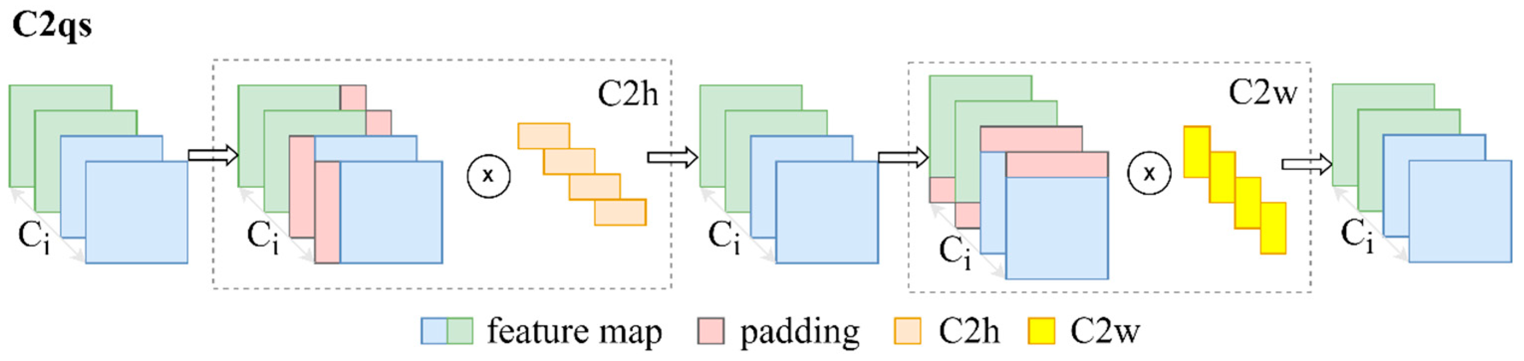
3.1. A 2 × 2 Convolution Kernel with Quadratic Separation and a New Symmetric Padding Strategy (C2qs)

In order to save computing resources, the C2qs convolution is designed. The detailed steps of C2qs are as follows. First, the standard 2 × 2 convolution kernel (C2) is channel separated in the horizontal and vertical directions, respectively, and the height convolution C2h (1 × 2) and width convolution C2w (2 × 1) are obtained. Then, a new symmetric padding strategy is used to alleviate the information shift problem.

Without changing the size of the feature map, due to the asymmetry of the receptive field of C2, the extracted feature map will have an information shift problem (moving to the upper left corner of the spatial position) when the simple C2 performs the convolution operation to extract features [24]. The receptive fields of C2h and C2w obtained from C2 separation also inherit the asymmetry, but their shift directions are separated into horizontal and vertical directions, respectively. Therefore, a new unilateral directional symmetric padding strategy is carried out for C2h or C2w in the horizontal or vertical directions, respectively, in this paper, so that the information receptive fields of C2h and C2w have symmetry.

For a single feature map, introducing symmetry in its convolution process is challenging. However, it is feasible to introduce symmetry in the feature map of the overall output for a single convolutional layer. For example, for C2h, under ideal conditions, the traditional zero-padding convolution operation causes the extracted feature map information to be shifted by 1 pixel. Upon performing $N$ traditional zero-padding convolution operations, the receptive fields of the horizontal shift $B_x$ gradually adds up. Assuming that $\alpha$ is the coordinate describing the pixel point in the feature map, the pixel shift in the feature map is shown in Equation (6).

$$F_0(\alpha )\to F_n[\alpha -(n,0)]$$

(6)

Assuming that the upper left pixel is used as the starting point, its shift includes two directions: left and right. The horizontal shift domain is shown in Equation (7).

$$B_x=\left\{\left.B_0,B_1\right\}\right.$$

(7)

By adjusting the scale of the left and right shift receptive fields, the overall output feature map can introduce symmetry in the convolution process of this layer. In other words, through left and right shift adjustment, the pixel shift can be ensured to return to the standard convolution state, as shown in Equation (8).

$$F_0(\alpha )\to F_n[\alpha ]$$

(8)

Assuming divisibility by 2 for the input channel $C_i$, the channel is partitioned into equal halves. Employing a left and right unilateral symmetric padding strategy in the horizontal direction on the feature maps in the group, followed by concatenation, results in their horizontal shifts canceling each other out and converging towards 0. This ensures strict adherence to symmetry within a single convolutional layer. When two shifted feature maps are combined within a sole convolutional layer, the receptive field of C2h experiences is partial extended, exemplified by $1\times 2\to 1\times 3$; thereby, its capability for information acquisition and representation is augmented. Similarly, for C2w, the input channel $C_i$ is divided into two equal parts, and the upper and lower unilateral directional symmetrical padding strategies are applied to the feature maps in the group in the vertical direction so that the vertical shift in the total amount tends to 0, thereby alleviating the problem of information shift. The symmetrical padding method is shown in Figure 1.

To sum up, the padding strategy of C2qs is divided into three steps. (1) The input feature maps are divided into two groups. (2) According to the direction defined in the grouping, the corresponding padding operation is carried out on the feature map in a single convolutional layer. (3) Upon completion of feature map concatenation, convolution calculations are performed (without padding).

Experimental results reveal that, although the accuracy of the C2qs slightly decreases in comparison to standard convolution, it exhibits fewer parameters and faster running speed. Two factors contribute to this. First, spatially separable convolution exhibits limited capability in extracting information along other directions, such as the diagonal, resulting in the loss of crucial information. This effect becomes more pronounced as the depth of the network increases. Second, a convolution kernel with a size of 2 × 2 has a smaller receptive field, leading to less acquisition of global feature information.

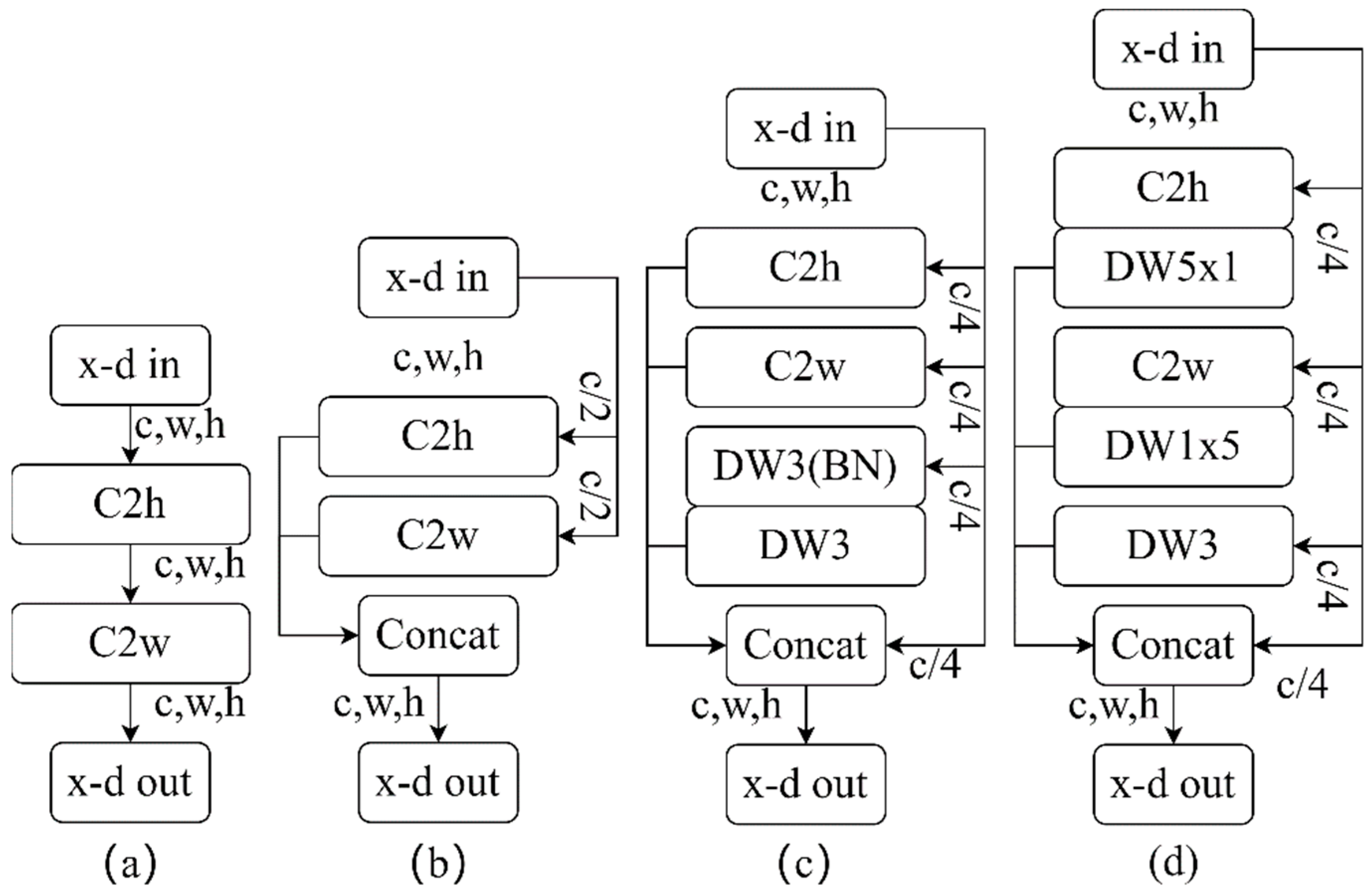
3.2. Multi-Scale Quadratic Separation Convolution Module (Mqscm)

Due to the inadequacy of C2qs in effectively balancing the tradeoff between network accuracy and speed, this paper presents further enhancements to C2qs and, ultimately, proposes a solution. The workflow of Mqscm is depicted in Figure 2. Its architecture shares similarities with group convolution and inception; however, the convolution kernels corresponding to each group in Mqscm are different. This distinction arises from the optimization of images with varying information distribution. Specifically, larger convolution kernels are favored for images with a more uniform information distribution, whereas images with a more localized information distribution prefer smaller convolution kernels. Mqscm employs convolution kernels of varying sizes to extract information across multiple scales, thereby ensuring network performance.

In an ideal scenario where the input and output tensors maintain the same size, under the assumption that the number of channels ($C$) is divisible by 4, Mqscm divides the learnable channel into four groups, resulting in four separated input groups $\left\{x_1,x_2,x_3,x_4\right\}$. Each group is assigned distinct convolution kernels, namely (C2h + DW5 × 1, C2w + DW1 × 5, DW3, 0), where DW (1 × 5, 5 × 1) represents the quadratic separation convolution. This convolution operation first separates the 5 × 5 convolution by channel and then by space, forming isomerism with C2h and C2w, respectively. The goal is to reduce information redundancy in the network space, capture both horizontal and vertical information, and attain a larger receptive field. $x_3$ undergoes a 3 × 3 depthwise convolution to extract feature information in other directions, such as the diagonal. $x_4$ undergoes no operations and is directly passed to $y_4$ to supplement detailed information of certain global features. Finally, the output results of each branch $\left\{y_1,y_2,y_3,y_4\right\}$ are concatenated.

Following the calculation method of standard convolution, the parameter count for Mqscm is $M=C(k^2+14)/4$ and the computation amount is $N=CWH(k^2+14)/4$. The calculation quantity ratio ($L$) between Mqscm and standard convolution is shown in Equation (9).

$$L=\frac{C(k^2+14)WH/4}{{(Ck)}^{2}WH}=\frac{(k^2+14)}{4C{k}^2}$$

(9)

In Equation (9), as $k$ approaches infinity, $L=1/(4C)$, and when $k$ is 1, $L=15/(4C)$. However, in practical neural networks, the number of channels $C$ is typically greater than 4. Consequently, the ratio consistently fulfills $L<1$, indicating that Mqscm has fewer parameters and memory overhead. Generally, in convolutional neural networks, the number of channels is commonly doubled, leading to a more significant reduction as the network deepens.

In summary, the Mqscm module has three advantages. First, it employs quadratic separation convolution to diminish the redundancy of network space information. Second, it utilizes kernels of different sizes to extract multi-scale information for fusion, enhancing the performance of convolutional blocks. Third, it expands the width and depth of the network. However, it also exhibits notable drawbacks. The multi-branch structure and unilateral directional symmetric padding operation increase network fragmentation, potentially diminishing the parallel speed of hardware computing. Furthermore, its information-capture capability requires enhancement. Future research directions may involve optimizing the fragmentation of the Mqscm module to accelerate speed and improve the ability to extract global details, thereby further advancing accuracy.

3.3. MqscmNet

The MqscmNet network architecture designed in this paper is improved, based on the non-bottleneck architecture ResNet-50 [13], and the network structure is shown in Figure 3a. It does not use any additional gain mechanism (such as an attention mechanism), but simply performs convolution replacement and model architecture simplification operations; the network can also obtain better efficiency tradeoff.

First, in the ResNet-50 architecture, the standard 3 × 3 convolution inside each residual block is replaced by an Mqscm module. Figure 3b shows the residual block formed by Mqscm. The main path is composed of dimensionality reduction point convolution (1 × 1), the Mqscm module, and dimensionality increase convolution (1 × 1) in series, and use the residual connection to add the input and output of the main path.and by using the residual connection, the input and the output of the main path are added. According to Formula (9), the number of parameters of Mqscm is far less than that of standard convolution, which can save a lot of computing resources and reduce memory overhead. For downsampling, DW 3 × 3 (s = 2, p = 1) convolution is directly used to replace the standard 3 × 3 convolution (s = 2, p = 1) in the original downsampling residual module, which further improves the speed. Similarly, the corresponding ratio L of Mqscm and standard convolution is shown in Equation (10).

$$L=\frac{23CWH/4}{9C^{2}WH}=\frac{23}{36C}$$

(10)

In Equation (10), as $C$ approaches infinity, $L$ converges to 0. Considering that $C$ is significantly greater than 1, $L$ consistently stays below 1. The replacement of the original subsampling module with this module can significantly reduce the computational cost of the network and increase the speed of network parallel computing. Second, for the purpose of network simplification, this study modifies the stacking frequency of residual blocks from (3, 4, 6, 3) to (2, 2, 6, 2). This adjustment not only significantly reduces the model parameters but also refines and compactifies the network architecture. Finally, the 7 × 7 convolution kernel with a step size of 2 in the initial layer of the network is substituted with a 4 × 4 convolution kernel with a step size of 2. Subsequently, the max-pooling layer in the second layer is replaced by a 2 × 2 convolution kernel with a step size of 2. This replacement strategy ensures the retention of more feature information, while simultaneously reducing the number of parameters.

4. Experiment and Analysis

As discussed in this section, an extensive array of experiments was conducted on three authentic datasets: CIFAR-10 [31], Tiny-ImageNet [6], and SVHN [32]. To study the influence of Mqscm on network performance without considering variously complex architectures and gain mechanisms, the bottleneck-free architecture model ResNet-50 [13] was selected. First, in this paper, only 3 × 3 standard convolution in each residual basic block was replaced, keeping the remaining relevant parameters unchanged for comparisons among multiple convolution blocks. Second, the stacking times of residual blocks in the model were adjusted to evaluate the performance of Mqscm under varying computational overheads. Subsequently, the MqscmNet network was constructed and comparative experiments were conducted with a series of classic networks, eliminating the interference of additional gain mechanisms and, more intuitively, demonstrating the impact of network simplification on performance. Finally, in the MqscmNet network, variations of Mqscm were compared and tested to verify the influence of different structures on the performance of the MqscmNet network. In addition, all architectures were implemented using PyTorch [33], and the experimental machine was equipped with an NVIDIA GeForce RTX 3060 graphics card.

4.1. Datasets and Training Settings

CIFAR-10: The CIFAR-10 dataset [31] is a small dataset designed for identifying ordinary objects, created by Alex Krizhevsky and Ilya Sutskever. It includes 60,000 color natural images sized at 32 × 32, divided into 10 categories. Each category contains an average of 6000 images, with 50,000 images allocated for training and 10,000 images for testing, ensuring no overlap in the dataset. In this paper, a standard data augmentation scheme was employed. First, an image-padding operation (padding = 4) was applied to resize the image to 40 × 40. Second, the image was randomly cropped to the size of 32 × 32, followed by random horizontal flipping and random occlusion. Finally, normalization was performed.

Tiny-ImageNet: The Tiny-ImageNet dataset [6] is a subset of ImageNet [34], with a total of 200 categories, with 500 images in each category as the training set, and 50 images as the validation set. It is a color image with a resolution of 64 × 64. The higher the resolution, the more complex the learning features and the longer the training time. This paper adopted the same image-enhancement method as that of CIFAR-10.

SVHN: The SVHN [32] dataset comprises a total of 10 categories, representing color digital images ranging from 0 to 9, with an image resolution of 32 × 32. The training set consists of 73,257 images, and the test set contains 26,032 images. The same image-enhancement method was applied.

Training setting: For all networks, the settings included batch size = 256, epoch = 100, and an initial learning rate (Lr) of 0.01. The SGD optimizer was employed to optimize gradient information, with a momentum of 0.9 and weight decay of 5 × 10⁻³, indicating a significant L2 regularization to mitigate overfitting. The learning rate (Lr) was adjusted using the step learning rate MultiStepLR, with Lr decreasing to 0.1 times the learning rate of the previous stage at 0.45× and 0.7× epochs, respectively. Batch normalization (BN) [35] was utilized to address the issue of gradient disappearance. ReLU was chosen as the activation function. The CIFAR-10 dataset, the Tiny-ImageNet dataset, and the SVHN dataset employed the same training settings.

4.2. Results and Analysis

This paper evaluates the performance of Mqscm on three public image-classification datasets, utilizing the bottleneck-free architecture ResNet-50 [13] to demonstrate that Mqscm enhances network performance without the need for additional gain mechanisms. We replaced each standard 3 × 3 convolution (Conv3) in the residual block with Mqscm, 3 × 3 depthwise convolution (DWConv3), or 2 × 2 convolution using a symmetric padding strategy (C2sp), respectively. Then, the performance of multiple convolution blocks was compared. All data processing and training details remained the same to ensure the fairness of the experiment.

Table 1. Performance comparison of several convolution modules on the CIFAR-10 dataset.

Convolution	FLOPs (M)	Params (M)	Accuracy (%)	Time/Epoch (s)
Conv3	84.34	23.53	89.17	48.61
DWConv3	46.85	12.25	88.49	30.60
C2sp	63.37	17.24	88.37	38.29
Mqscm	46.77	12.24	88.56	32.81

shows the classification results of Mqscm, Conv3, DWConv3, and C2sp convolution on the CIFAR-10 dataset. In this paper, the metrics compared were computing complexity (FLOPs), parameter size (Params), accuracy, and average training time per epoch (Time/Epoch). Ranked by computational complexity, Conv3 > C2sp > DWConv3 > Mqscm. Ranked by accuracy, Conv3 > Mqscm > DWConv3 > C2sp. Ranked by speed, DWConv3 > Mqscm > C2sp > Conv3. The standard convolution Conv3 had, undoubtedly, the highest accuracy, but it had the largest computational complexity, the largest number of parameters, and the longest training time. DWConv3 was the fastest and achieved a good efficiency tradeoff, but the computational complexity and accuracy were slightly lower than those of Mqscm. C2sp performed well but was weaker than Mqscm in all aspects. This is attributed to the heightened sensitivity of standard convolution to the complex feature information in images and its robust representation capability. However, the simultaneous consideration of channels and regions contributed to increased computing and memory requirements, thereby impacting the efficiency of network training. Conversely, DWConv3 and Mqscm effectively reduced the number of parameters and enhanced training speed through distinct separation methods. Nevertheless, there was a tradeoff, as they occasionally lost some global information, leading to a slight decrease in accuracy. Compared with Conv3, Mqscm saved about 44.5% of the calculated amount and accelerated the model training by about 32.5%. The comprehensive performance of Mqscm was comparable to that of DWConv3.

Table 2. Performance comparison of several convolution modules on the Tiny-ImageNet dataset.

Convolution	FLOPs (M)	Params (M)	Accuracy (%)	Time/Epoch (s)
Conv3	337.69	23.91	54.38	97.44
DWConv3	187.71	12.63	55.46	73.75
C2sp	253.81	17.63	53.59	99.83
Mqscm	187.39	12.63	56.20	82.89

presents the classification performance comparison of several convolution methods on the Tiny-ImageNet dataset. It is evident that Mqscm outperformed the other convolutional modules in the Table in terms of FLOPs, Params, and accuracy, and it trained faster than Conv3 and C2sp, and just below DWConv3. This occurred because the substantial extraction of intricate information by the standard convolution method obscured some crucial details in this dataset, leading to lower accuracy in Conv3 and C2sp compared to that of Mqscm and DWConv3. The unique structure of Mqscm not only diminished information redundancy but also integrated multi-scale information, resulting in optimal accuracy for this dataset. Compared to Conv3, Mqscm improved accuracy by 1.82% and enhanced model training speed by 14.93%.

Table 3. Performance comparison of several convolution modules on the SVHN dataset.

Convolution	FLOPs (M)	Params (M)	Accuracy (%)	Time/Epoch (s)
Conv3	84.34	23.53	96.51	72.602
DWConv3	46.85	12.25	96.13	43.18
C2sp	63.37	17.24	96.17	55.45
Mqscm	46.77	12.24	96.22	46.89

shows the classification performance comparison of several convolution modules on the SVHN dataset. It is evident that Mqscm exhibited the fewest FLOPs (M) and Params (M) and surpassed Conv3 and C2sp in terms of training time. This is attributed to Mqscm’s reduction in computing and memory requirements through secondary separation, consequently enhancing the training efficiency of the network. In terms of accuracy, it outperformed DWConv3 and C2sp, because Mqscm integrated multi-scale information, to some extent mitigating the issue of global information loss resulting from secondary separation. Compared with Conv3, the model speed improved by 35.41%. The experiments demonstrated that the performance of Mqscm on SVHN datasets was highly competitive and comparable to that of depthwise separable convolution.

In summary, Mqscm only requires a direct replacement of the original standard convolution, resulting in substantial savings in computational resources and memory overhead. Moreover, it accelerates model training while maintaining a high level of accuracy. Experiments conducted on three real public datasets demonstrated that Mqscm not only effectively achieved efficiency tradeoffs in networks, but also exhibited good generalization.

This paper provides tradeoff curves of accuracy and speed under different FLOPs on the CIFAR-10 dataset, as shown in Figure 4. Subgraph (a) displays the accuracy tradeoff curve under different FLOPs and subgraph (b) illustrates the speed tradeoff curve under different FLOPs.

In ResNet-50, the stacking times of blocks from stage 1 to stage 4 are (3, 4, 6, 3). In this paper, the stacking times were changed to (1, 1, 3, 1) and (2, 2, 6, 2) to achieve different computational complexity and parameters, while the remaining settings remained unchanged. The experimental results indicated that Mqscm achieved faster speeds than Conv3 and C2sp, while maintaining higher accuracy than DWConv3 across various computational complexities and parameters, all without the need for additional gain mechanisms such as attention mechanisms. In summary, Mqscm exhibited an overall performance comparable to that of depthwise separable convolution, striking a good balance between accuracy and network efficiency.

To further explore the performance of Mqscm, this paper proposes a straightforward convolutional network, MqscmNet, with a simple architecture, as illustrated in Figure 3. In

Table 4. Performance comparison of MqscmNet and classical networks on the CIFAR-10 dataset.

Net	FLOPs (M)	Params (M)	Accuracy (%)	Time/Epoch (s)
AlexNet	67.08	3.75	83.47	28.79
Vgg-16	1257.21	29.45	94.23	42.79
GoogleNet	32.55	5.99	88.67	32.93
Mobilenet_v3_Small	2.28	1.52	73.52	27.64
Mobilenet_v3_large	7.45	4.21	84.34	29.08
ResNet-50	84.34	23.53	89.17	48.61
ResNet-50+Mqscm	46.76	12.24	88.56	32.75
MqscmNet	40.63	9.54	89.76	34.19

, this subsection presents the performance comparison experiment of various classical classification networks on the CIFAR-10 dataset. To ensure fairness, BN regularization was employed to mitigate the gradient-disappearance problem in these networks, and the activation function uniformly used Relu. The experimental results showed that the accuracy of MqscmNet was only lower than that of Vgg-16 and was much higher than that of other classical networks. Compared with ResNet-50, MqscmNet had fewer network layers, the parameters were reduced by about 59.5%, the training time was reduced by about 29.7%, and the accuracy was increased by 0.59%. This arose due to task-specific challenges, where the excessive depth of ResNet-50 network layers resulted in repeated extraction of complex information, masking certain details. In contrast, MqscmNet simplified the number of network layers and used Mqscm to widen the network and reduce computational workload and memory overhead. This strategy improved the accuracy and efficiency of the network.

It was found that reducing the computational load was only a necessary condition, but not a sufficient condition for achieving network lightweightness. For example, the computational load and parameters of Vgg-16 were larger than those of ResNet-50, but Vgg-16 had higher accuracy and faster speed. These experimental findings affirmed that MqscmNet effectively leveraged the performance of Mqscm and balanced the relationship between network speed and accuracy.

Table 5. Performance comparison of different Mqscm structures on the CIFAR-10 dataset.

Model	Design	FLOPs (M)	Params (M)	Accuracy (%)	Time/Epoch (s)
ResNet-50	Mqscm-a	46.72	12.23	88.12	31.50
	Mqscm-b	46.67	12.23	88.15	31.38
	Mqscm-c	46.79	12.23	88.27	32.97
	Mqscm-d	46.77	12.24	88.56	32.81
MqscmNet	Mqscm-a	40.59	9.53	89.21	33.63
	Mqscm-b	40.54	9.53	89.25	33.22
	Mqscm-c	40.65	9.53	89.28	34.33
	Mqscm-d	40.63	9.54	89.76	34.19

presents comparative experiments involving several variant structures of Mqscm on the CIFAR-10 dataset, with their structures depicted in Figure 5. ResNet-50 and MqscmNet network structures were utilized to assess the impact of different structures on accuracy and speed. The experimental results showed that among the four structures, Mqscm-d had the highest accuracy, but the training speed was slightly slower than that of Mqscm-b. This is because Mqscm-d enhanced the accuracy of the model through the multi-scale structure, but also increased the degree of fragmentation, potentially reducing the parallel speed of the hardware. Mqscm-b trained the fastest but with less accuracy. All four variants of Mqscm showed superior performance in MqscmNet networks compared to ResNet-50, which confirmed the effectiveness of MqscmNet in enhancing performance.

It is evident from Table 1, Table 2 and Table 3 that DWConv3 exhibited performance characteristics that were highly similar to those of Mqscm. To conduct a more in-depth performance comparison, two widely recognized architectures, namely ResNet-50 and Mobilenet_v3_large, were employed for k-fold cross-validation across three datasets. The training set was divided into five subsets, and the models underwent evaluation and training five times, followed by testing on the respective test sets.

Table 6. The accuracy comparison of Mqscm and DWConv3 through k-fold cross-validation.

				Accuracy (%)
Net	Convolution	CIFAR-10	Tiny-ImageNet	SVHN
ResNet-50	DWConv3	88.61	55.92	96.27
	Mqscm	88.85	56.39	96.35
Mobilenet_v3_large	DWConv3	84.52	26.60	93.79
	Mqscm	84.66	26.95	93.85

presents the accuracy comparison of Mqscm and DWConv3 through k-fold cross-validation.

The data presented in Table 6 reveal that Mqscm exhibited superior accuracy compared to that of DWConv3 across three datasets and two distinct classic architectures. This superiority can be attributed to the multi-scale topology inherent in Mqscm, which enhanced its information-extraction capabilities. Furthermore, it is noteworthy that both Mqscm and DWConv3 achieved higher accuracy in the context of ResNet-50 compared to Mobilenet_v3_large. This discrepancy arose from the fact that ResNet-50, with its deeper network architecture, extracted more intricate feature information, whereas Mobilenet_v3_large, a classic lightweight architecture, significantly reduced FLOPs and Params at the cost of sacrificing a portion of its information-extraction capability. In summary, across the three data scenarios presented in Table 6, Mqscm consistently outperformed DWConv3 in terms of accuracy.

5. Conclusions

This paper explored a convolutional block, Mqscm, that meets the requirements of lightweight design and uses it to construct MqscmNet, a network with a relatively simple architecture. Experimental results on real datasets showed that, compared with Conv3, Mqscm can save 44.5% of the computational cost and 47.9% of the parameter count, and the model training speed improves by a range of 14.93% to 35.41% while maintaining competitive accuracy. The comprehensive performance is comparable to that of depthwise separable convolution. Compared with C2sp, Mqscm saves 26.2% of the computation and 29% of the parameter count, with a 14.3% reduction in training time and a slight improvement in accuracy. In comparison with ResNet-50, MqscmNet reduces parameters by about 59.5% and training time by about 29.7%, and improves accuracy by 0.59%. The substantial reduction in the number of network layers significantly improves the efficiency tradeoff.

In summary, the contributions of this paper are as follows.

(1) Aiming at the problem of numerous parameters and low efficiency of the network model, the C2qs module was proposed in this paper. The module combines depth-separable and space-separable methods to separate 2 × 2 convolution. This operation effectively reduces the number of FLOPs and Params in the network and shortens the training time. In addition, a new symmetric filling method was designed to alleviate the information-shift problem of even-convolution kernels.

(2) Since the quadratic separation method may cause some global information to be lost, we built the Mqscm module. This module uses convolution kernels of different sizes to extract multi-scale information for fusion to make up for the decline in network performance due to partial information loss. In addition, the four-branch topology increases the network width and improves network performance to a certain extent.

(3) A pure convolutional network MqscmNet was constructed using the Mqscm module, and compared with classical networks such as AlexNet, VGG-16, GoogleNet, MobileNet, and ResNet-50. MqscmNet achieved accuracy similar to or higher than that of the classical networks, while having fewer parameters and a faster training time, proving its effectiveness in balancing speed and accuracy.

(4) Experiments were conducted on three datasets to assess the performance of various convolution techniques. The results indicated that Mqscm is an effective decomposition method for Conv3, which can save 44.5% of the FLOPs and 47.9% of the Params. In addition, training time was reduced, and accuracy was maintained. In comparing various Mqscm variants, the experimental analysis revealed that an increase in Mqscm branches corresponded to greater accuracy. However, this was accompanied by an increase in training time. This showed that the degree of fragmentation of the network affects the efficiency of the network.

(5) This work provides valuable insights into future research on lightweight neural networks, providing a compelling alternative for developing efficient convolutional modules.

References

1. Vargas-Hakim, G.-A.; Mezura-Montes, E.; Acosta-Mesa, H.-G. A Review on Convolutional Neural Networks Encodings for Neuroevolution. IEEE Trans. Evol. Comput. 2021, 26, 12–27. [Google Scholar] [CrossRef]
2. Gómez-Guzmán, M.A.; Jiménez-Beristaín, L.; García-Guerrero, E.E.; López-Bonilla, O.R.; Tamayo-Perez, U.J.; Esqueda-Elizondo, J.J.; Palomino-Vizcaino, K.; Inzunza-González, E. Classifying Brain Tumors on Magnetic Resonance Imaging by Using Convolutional Neural Networks. Electronics 2023, 12, 955. [Google Scholar] [CrossRef]
3. Weng, L.; Wang, Y.; Gao, F. Traffic scene perception based on joint object detection and semantic segmentation. Neural Process. Lett. 2022, 54, 5333–5349. [Google Scholar] [CrossRef]
4. Li, S.; Liu, Y.; Zhang, Y.; Luo, Y.; Liu, J. Adaptive Generation of Weakly Supervised Semantic Segmentation for Object Detection. Neural Process. Lett. 2023, 55, 657–670. [Google Scholar] [CrossRef]
5. Krizhevsky, A.; Sutskever, I.; Hinton, G.E. ImageNet classification with deep convolutional neural networks. Commun. ACM 2017, 60, 84–90. [Google Scholar] [CrossRef]
6. Russakovsky, O.; Deng, J.; Su, H.; Krause, J.; Satheesh, S.; Ma, S.; Huang, Z.; Karpathy, A.; Khosla, A.; Bernstein, M.; et al. Imagenet large scale visual recognition challenge. Int. J. Comput. Vis. 2015, 115, 211–252. [Google Scholar] [CrossRef]
7. Liu, Z.; Mao, H.; Wu, C.Y.; Feichtenhofer, C.; Darrell, T.; Xie, S. A convnet for the 2020s. In Proceedings of the IEEE/CVF Conference on Computer Vision and Pattern Recognition, New Orleans, LA, USA, 18–24 June 2022; pp. 11976–11986. [Google Scholar]
8. Simonyan, K.; Zisserman, A. Very deep convolutional networks for large-scale image recognition. arXiv 2014, arXiv:1409.1556. [Google Scholar]
9. Szegedy, C.; Liu, W.; Jia, Y.; Sermanet, P.; Reed, S.; Anguelov, D.; Erhan, D.; Vanhoucke, V.; Rabinovich, A. Going deeper with convolutions. In Proceedings of the IEEE Conference on Computer Vision and Pattern Recognition, Boston, MA, USA, 7–12 June 2015; pp. 1–9. [Google Scholar]
10. Szegedy, C.; Ioffe, S.; Vanhoucke, V.; Alemi, A. Inception-v4, inception-resnet and the impact of residual connections on learning. In Proceedings of the AAAI Conference on Artificial Intelligence, San Francisco, CA, USA, 4–9 February 2017; Volume 31. [Google Scholar]
11. Szegedy, C.; Vanhoucke, V.; Ioffe, S.; Shlens, J.; Wojna, Z. Rethinking the inception architecture for computer vision. In Proceedings of the IEEE Conference on Computer Vision and Pattern Recognition, Las Vegas, NV, USA, 27–30 June 2016; pp. 2818–2826. [Google Scholar]
12. He, K.; Zhang, X.; Ren, S.; Sun, J. Identity Mappings in Deep Residual Networks; Springer: Cham, Switzerland, 2016; pp. 630–645. [Google Scholar]
13. He, K.; Zhang, X.; Ren, S.; Sun, J. Deep residual learning for image recognition. In Proceedings of the IEEE Conference on Computer Vision and Pattern Recognition, Las Vegas, NV, USA, 27–30 June 2016; pp. 770–778. [Google Scholar]
14. Xie, S.; Girshick, R.; Dollár, P.; Tu, Z.; He, K. Aggregated residual transformations for deep neural networks. In Proceedings of the IEEE Conference on Computer Vision and Pattern Recognition, Honolulu, HI, USA, 21–26 July 2017; pp. 1492–1500. [Google Scholar]
15. Kamarudin, M.H.; Ismail, Z.H.; Saidi, N.B.; Hanada, K. An augmented attention-based lightweight CNN model for plant water stress detection. Appl. Intell. 2023, 53, 1–16. [Google Scholar] [CrossRef]
16. Pintelas, E.; Livieris, I.E.; Kotsiantis, S.; Pintelas, P. A multi-view-CNN framework for deep representation learning in image classification. Comput. Vis. Image Underst. 2023, 232, 103687. [Google Scholar] [CrossRef]
17. Bonam, J.; Kondapalli, S.S.; Prasad, L.V.N.; Marlapalli, K. Lightweight CNN Models for Product Defect Detection with Edge Computing in Manufacturing Industries. J. Sci. Ind. Res. 2023, 82, 418–425. [Google Scholar]
18. Liu, D.; Zhang, J.; Li, T.; Qi, Y.; Wu, Y.; Zhang, Y. A Lightweight Object Detection and Recognition Method Based on Light Global-Local Module for Remote Sensing Images. IEEE Geosci. Remote Sens. Lett. 2023, 20, 1–5. [Google Scholar] [CrossRef]
19. Ye, Z.; Li, C.; Liu, Q.; Bai, L.; Fowler, J.E. Computationally Lightweight Hyperspectral Image Classification Using a Multiscale Depthwise Convolutional Network with Channel Attention. IEEE Geosci. Remote Sens. Lett. 2023, 20, 1–5. [Google Scholar] [CrossRef]
20. Wu, B.; Wan, A.; Yue, X.; Jin, P.; Zhao, S.; Golmant, N.; Gholaminejad, A.; Gonzalez, J.; Keutzer, K. Shift: A zero flop, zero parameter alternative to spatial convolutions. In Proceedings of the IEEE Conference on Computer Vision and Pattern Recognition, Salt Lake City, UT, USA, 18–23 June 2018; pp. 9127–9135. [Google Scholar]
21. Chollet, F. Xception: Deep learning with depthwise separable convolutions. In Proceedings of the IEEE Conference on Computer Vision and Pattern Recognition, Honolulu, HI, USA, 21–26 July 2017; pp. 1251–1258. [Google Scholar]
22. Gholami, A.; Kwon, K.; Wu, B.; Tai, Z.; Yue, X.; Jin, P.; Zhao, S.; Keutzer, K. Squeezenext: Hardware-aware neural network design. In Proceedings of the IEEE Conference on Computer Vision and Pattern Recognition Workshops, Salt Lake City, UT, USA, 18–23 June 2018; pp. 1638–1647. [Google Scholar]
23. Wu, S.; Wang, G.; Tang, P.; Chen, F.; Shi, L. Convolution with even-sized kernels and symmetric padding. In Proceedings of the Advances in Neural Information Processing Systems 32 (NeurIPS 2019), Vancouver, BC, Canada, 8–14 December 2019. [Google Scholar]
24. Chen, J.; Lu, Z.; Liao, Q. XSepConv: Extremely separated convolution. arXiv 2020, arXiv:2002.12046. [Google Scholar]
25. Yang, S.; Wen, J.; Fan, J. Ghost shuffle lightweight pose network with effective feature representation and learning for human pose estimation. IET Comput. Vis. 2022, 16, 525–540. [Google Scholar] [CrossRef]
26. Cao, J.; Li, Y.; Sun, M.; Chen, Y.; Lischinski, D.; Cohen-Or, D.; Chen, B.; Tu, C. Do-conv: Depthwise over-parameterized convolutional layer. IEEE Trans. Image Process. 2022, 31, 3726–3736. [Google Scholar] [CrossRef] [PubMed]
27. Li, X.; Yang, H.; Yang, C. ResE: A Fast and Efficient Neural Network-Based Method for Link Prediction. Electronics 2023, 12, 1919. [Google Scholar] [CrossRef]
28. Cui, B.; Dong, X.-M.; Zhan, Q.; Peng, J.; Sun, W. LiteDepthwiseNet: A lightweight network for hyperspectral image classification. IEEE Trans. Geosci. Remote Sens. 2021, 60, 1–15. [Google Scholar] [CrossRef]
29. Liu, J.J.; Hou, Q.; Cheng, M.M.; Wang, C.; Feng, J. Improving convolutional networks with self-calibrated convolutions. In Proceedings of the IEEE/CVF Conference on Computer Vision and Pattern Recognition, Seattle, WA, USA, 13–19 June 2020; pp. 10096–10105. [Google Scholar]
30. Howard, A.; Sandler, M.; Chu, G.; Chen, L.C.; Chen, B.; Tan, M.; Wang, W.; Zhu, Y.; Pang, R.; Vasudevan, V.; et al. Searching for mobilenetv3. In Proceedings of the IEEE/CVF International Conference on Computer Vision, Seoul, Republic of Korea, 28–29 October 2019; pp. 1314–1324. [Google Scholar]
31. Krizhevsky, A.; Hinton, G. Learning Multiple Layers of Features from Tiny Images. 2009. Available online: www.cs.utoronto.ca/~kriz/learning-features-2009-TR.pdf (accessed on 5 February 2023).
32. Netzer, Y.; Wang, T.; Coates, A.; Bissacco, A.; Wu, B.; Ng, A.Y. Reading Digits in Natural Images with Unsupervised Feature Learning. 2011. Available online: https://research.google/pubs/pub37648/ (accessed on 5 February 2023).
33. Haq, S.I.U.; Tahir, M.N.; Lan, Y. Weed Detection in Wheat Crops Using Image Analysis and Artificial Intelligence (AI). Appl. Sci. 2023, 13, 8840. [Google Scholar] [CrossRef]
34. Rohlfs, C. Problem-dependent attention and effort in neural networks with applications to image resolution and model selection. Image Vis. Comput. 2023, 135, 104696. [Google Scholar] [CrossRef]
35. Ioffe, S.; Szegedy, C. Batch normalization: Accelerating deep network training by reducing internal covariate shift. In Proceedings of the International Conference on Machine Learning, Lille, France, 6–11 July 2015; pp. 448–456. [Google Scholar]
Figure 1. Symmetric padding strategy for C2qs (C2h, C2w) convolution.
Electronics 12 04839 g001
Figure 2. Mqscm module using multiple quadratic separation convolution kernels.
Electronics 12 04839 g002
Figure 3. The overall structure of MqscmNet: (a) MqscmNet structure; (b) Mqscm residual block; (c) downsampling module.
Electronics 12 04839 g003aElectronics 12 04839 g003b
Figure 4. Convolutional tradeoff curves on CIFAR-10 dataset: (a) tradeoff curve of accuracy under different FLOPs; (b) tradeoff curve of speed under different FLOPs.
Electronics 12 04839 g004
Figure 5. Variant structure diagram of Mqscm: (a) Mqscm-a structure; (b) Mqscm-b structure; (c) Mqscm-c structure; (d) Mqscm-d structure.
Electronics 12 04839 g005