A Fault Location Method for Medium Voltage Distribution Network Based on Ground Fault Transfer Device

Abstract

The arc suppression device based on ground fault transfer (GFT) has been preliminarily applied in the medium voltage distribution network (MVDN). An accurate travelling wave (TW) fault location method is proposed to extend the use of the ground fault transfer device. D-PMU is used as a travelling wave detection tool to record the transient voltage travelling waves of fault grounding and bus active grounding during arc suppression. Then, the faulty section is identified through the time difference of travelling wave arrival at the upstream and downstream measurement points. On this basis, the fault location equations of the arrival time and distance of the upstream travelling wave are established, and an accurate fault location method based on the arrival time difference of the travelling wave is proposed. The simulation model is established by PSCAD/EMTDC, and the results show that the method has high location accuracy, and the absolute error is less than 30 m. It is not affected by the TW velocity, the fault conditions, or the distributed power sources.

1. Introduction

The GFT device was first used in the chemical industry, metallurgy, and other fields [1]. Later, because the fault current was too large and accompanied by overvoltage when a single-phase grounding fault occurred in the wind farm, the arc suppression coil alone could not provide a sufficient compensation current, so the neutral grounding mode was changed and the GFT device was introduced. With the increase in MVDN capacity and the popularization and use of cable lines, MVDNs such as wind farms generally encounter the above problems. The voltage arc extinguishing scheme is adopted due to its good arc extinguishing performance, and the arc extinguishing effect of related devices has also been verified in field tests [2].

In Reference [3], the field fault treatment test of the GFT device was carried out, and the fault treatment data were compared with the treatment results of the automatic tracking arc suppression compensation device, which verified the effectiveness of the fault treatment of the voltage arc extinguishing scheme. Reference [4] analyzed the dynamic characteristics of the grounding switch by the equivalent circuit method and optimized the design and parameter analysis of the fast arc suppression device. On this basis, the parameters of grounding intermediate resistance and grounding transformer were optimized in reference [5] and verified by the online operation data of the product. In Reference [6], the current transfer performance and overvoltage suppression ability of the transfer arc extinguishing device were studied, and the influence of load on the transfer arc extinguishing technology was analyzed. Reference [7] identified whether the fault point disappeared based on the difference in electrical quantities in the station for the light load and heavy load of the line, which provided a theoretical basis for the improvement of the control method of the fault transfer device. Correspondingly, the GFT device manufactured by the equipment manufacturer has been applied in the engineering field. For example, the intelligent disposal scheme of a single-phase grounding fault in an MVDN developed by the Shaanxi Electric Power Research Institute of China can effectively solve the problem of error correction and suppress the transient process, and it has good adaptability to high resistance grounding.

At present, the research work on GFT mostly focuses on the feasibility of the voltage arc extinguishing scheme and the transfer grounding device itself, and the fault location method matching with it is less involved. Making full use of fault information to achieve the accurate location of fault points can reduce the scope of manual line patrol and shorten the power outage times of end users [8], which is also considered to be one of the key measures when building an elastic power grid [9].

According to the different principles, the current fault location methods mainly include the impedance method and the travelling wave method. The impedance method establishes a location equation based on line parameters and measurement information and determines the exact distance of the fault by solving the equation [10]. Based on the distributed parameter model of the MVDN, Reference [11] constructs the location function with the current measurement information before and after the fault, which further improves the location accuracy. In Reference [12], the electrical parameters of the opposite end and the fault distance are taken as the quantities to be solved, and the parameter identification is carried out in combination with the spectrum information of the transient voltage and current. It is simple and reliable and overcomes the disadvantage that the single-ended location is easily affected by the system impedance in the traditional scheme. Reference [13] proposes an improved algorithm based on phasor analysis and a voltage and current calculation method suitable for an active MVDN, which can withstand certain load fluctuations.

Fault location based on TW information mainly uses the TW velocity and the arrival time of the wave head to determine the fault location. Theoretically, it is not affected by factors such as the system operation mode, fault type, or transition resistance [14,15], and the location accuracy is high. According to the location principle, it can be divided into the single-ended method [16], double-ended method [17], and modulus time difference method [18]. The single-ended method uses the time difference between the initial TW of the fault and the reflected TW of the fault point to construct the distance equation. The principle is simple and easy to implement, but the reflected wave head identification is more difficult [15]. The double-ended method calculates the fault distance according to the time difference between the initial TW and the MPs at both ends of the line. It only needs to capture the initial TW head but needs to arrange MPs at all branch nodes, and it needs to strictly meet the requirements of clock synchronization [19].

A new TW fault location method is proposed for the MVDN with a GFT device. Combined with the working characteristics of the GFT device, the arrival time of the TW head of the whole network is integrated when the fault is grounded and the bus is grounded. The fault location equation is constructed according to the arrival time difference of the travelling wave in the faulty section, the fault information of the upstream segment, and the line parameters. Because the location equation is independent of the wave velocity, the influence of the TW velocity on the location result is avoided. The simulation results show that the proposed method has high location accuracy, the absolute error is less than 30 m, and it has good location performance in different fault positions and fault conditions.

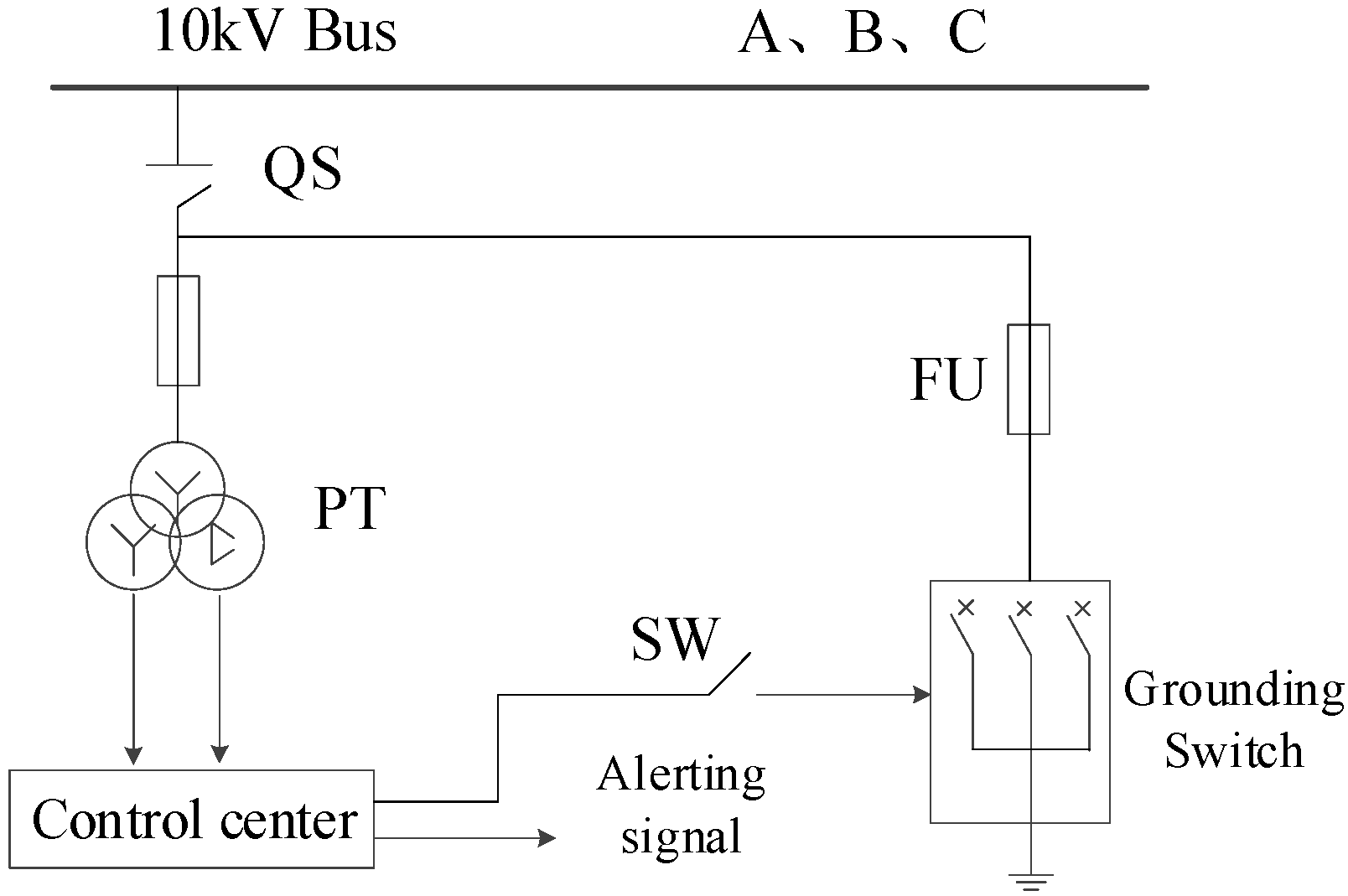
2. The Working Principle of the GFT Device

The GFT device [20] is generally implemented in the neutral point ungrounded system, which is connected to the substation bus through the outlet circuit breaker. The main components are the ground transformer, the control center, and the ground switch, which can be separated. The structure diagram is shown in Figure 1. In particular, different from the traditional circuit breaker using mechanical or electromagnetic suction to design the action switch, due to the need for rapid arc extinguishing, the device generally uses a Thomson coil as the action switch and uses electromagnetic repulsion to meet the requirements of the switch execution speed [21].

After determining the grounding fault of the system, the closing pulse is sent to the grounding switch of the faulty phase bus bar, so that the faulty phase bus bar is grounded quickly; the fault point is bypassed, so that the voltage of the fault point is clamped to close to 0, and the grounding arc can be effectively extinguished. After a short delay, the switch is disconnected, and whether the fault disappears is judged according to the zero sequence voltage. If it is a transient grounding fault, the fault disappears and the system returns to normal operation. Otherwise, it is judged to be a permanent fault, and the bus grounding switch is closed again. The scheme does not need to consider the problem of system-to-ground capacitive current and compensation capacity, and the arc extinguishing effect is remarkable. At the same time, after the action of the fault transfer device, the arc grounding that originally occurred on the line can be transformed into a metal grounding in the substation to avoid the formation of step voltage outside the station and reduce the risk of personnel accidents. However, the insulation of the line may be broken after a fault occurs. To avoid the recurrence of the fault, fault location should be carried out as soon as possible to realize the isolation of the nearest fault point.

In the process of fault arc suppression, there are two transient processes of fault grounding and faulty phase bus grounding, so the same line also has two types of transient information, before and after, which provides a new idea for the research of fault location. Taking the TW fault location method studied in this paper as an example, when the GFT device acts, it is equivalent to creating a second grounding fault at the busbar. The arrival time of the line grounding TW can be combined with the arrival time of the busbar grounding TW to construct a new location equation.

3. Accurate Fault Location Method Based on TWATD

Considering the serious attenuation of zero-mode TW, aerial-mode TW is often used in the calculation of the TW location, but the acquisition of the aerial-mode wave velocity also needs to be matched with accurate line parameters. For the MVDN with the same voltage level, when the frequency is high enough, the aerial-mode wave velocity at the same frequency can be regarded as a certain value [22]. Therefore, the same high-frequency modulus TW can be used for location calculation to avoid the error caused by inconsistent wave velocity. To achieve this goal, the extracted TWs should be at the same frequency. At present, there are many research results on the detection of the TW head, among which the wavelet transform is widely used. However, the analysis scale and wavelet basis function need to be selected according to the fault characteristics, and the extraction range is limited to a certain frequency band, so it is impossible to extract the TW signal with a single frequency. Based on the Morlet wavelet, the S transform solves the problem that the frequency of the STFT window cannot be adjusted, and it has the advantage of multi-resolution of the wavelet transform [23]. Therefore, this paper uses the S transform to identify the fault TW head. There are many papers that introduce the algorithm [24,25], so the details are not repeated in this paper.

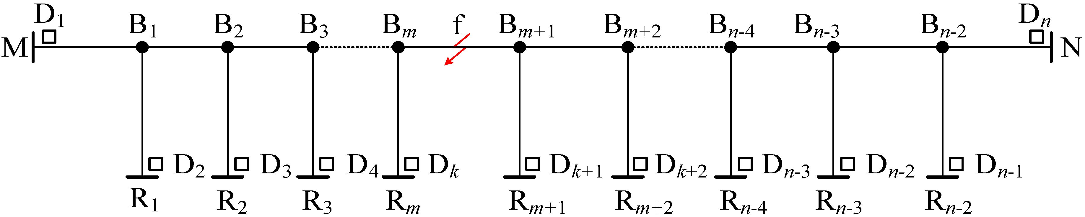
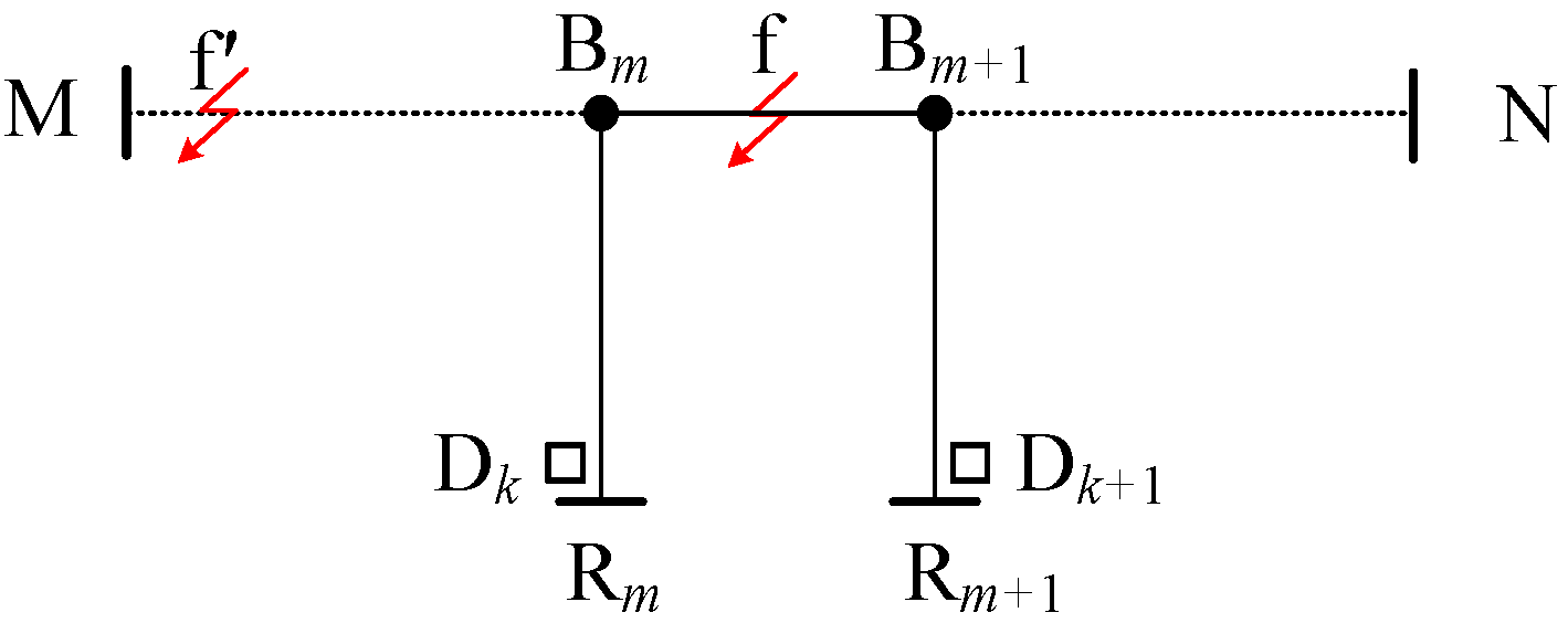
3.1. Faulty Section Identification Method

For the situation in which the line experiences a grounding fault, the MVDN shown in Figure 2 can be taken as an example; the power supply, transformer, and load are omitted in the figure. Among them, MN is the main trunk line, and the branch line BR is connected to the trunk line with branch point B. D_k represents the MPs, which are arranged at the end of the network; B_m represents the branch point; and R_m represents the network endpoint.

Assuming that the branch ${\mathrm{B}}_m{\mathrm{B}}_{m+1}$ experiences a ground fault, the entire network can be divided into two parts according to the location of the fault point, where the end point M and the branch point ${\mathrm{B}}_m$ surrounding area are called the upstream section, and the end point N and the branch point ${\mathrm{B}}_{m+1}$ surrounding area are called the downstream section. Assuming that the fault initial TW detected at each MP is taken from the same higher frequency, the TW velocity of each line is consistent, and the TW transmission equation can be written for the upstream MP:

$$\left[\begin{array}{c}{t}_{{\mathrm{D}}_1}\\ ⋮\\ t_{{\mathrm{D}}_i}\\ ⋮\\ t_{{\mathrm{D}}_k}\end{array}\right]=\frac{1}{v}\left[\begin{array}{c}{l}_{{\mathrm{D}}_1{\mathrm{B}}_m}+l_{{\mathrm{fB}}_m}\\ ⋮\\ l_{{\mathrm{D}}_i{\mathrm{B}}_m}+l_{{\mathrm{fB}}_m}\\ ⋮\\ l_{{\mathrm{D}}_k{\mathrm{B}}_m}+l_{{\mathrm{fB}}_m}\end{array}\right]+t_{\mathrm{f}}\left[\begin{array}{c}1\\ ⋮\\ 1\\ ⋮\\ 1\end{array}\right]$$

(1)

where $t_{{\mathrm{D}}_i}$ is the time at which the initial TW of the fault arrives at the MP D_i, $l_{{\mathrm{D}}_i{\mathrm{B}}_m}$ is the distance between the MP D_i and the branch point B_m, v is the speed at which the travelling wave travels through the line, $l_{{\mathrm{fB}}_m}$ is the distance between the branch point B_m and the fault point f, and $t_{\mathrm{f}}$ is the time at which the fault occurs.

By subtracting the adjacent equations in Equation (1) and eliminating the time of the fault, we have

$$\left[\begin{array}{l}{t}_{{\mathrm{D}}_1}-t_{{\mathrm{D}}_2}\\ t_{{\mathrm{D}}_2}-t_{{\mathrm{D}}_3}\\ \cdots \\ t_{{\mathrm{D}}_i}-t_{{\mathrm{D}}_{i+1}}\\ \cdots \\ t_{{\mathrm{D}}_{k-1}}-t_{{\mathrm{D}}_k}\end{array}\right]=\frac{1}{v}\left[\begin{array}{c}{l}_{{\mathrm{B}}_1{\mathrm{D}}_1}-l_{{\mathrm{B}}_1{\mathrm{D}}_2}\\ l_{{\mathrm{B}}_2{\mathrm{D}}_2}-l_{{\mathrm{B}}_2{\mathrm{D}}_3}\\ \cdots \\ l_{{\mathrm{B}}_i{\mathrm{D}}_i}-l_{{\mathrm{B}}_i{\mathrm{D}}_{i+1}}\\ \cdots \\ l_{{\mathrm{B}}_{{}_{k-1}}{\mathrm{D}}_{{}_{k-1}}}-l_{{\mathrm{B}}_{{}_{k-1}}{\mathrm{D}}_k}\end{array}\right]$$

(2)

Similarly, for each MP in the downstream region, the following results can be obtained:

$$\left[\begin{array}{l}{t}_{{\mathrm{D}}_{k+1}}-t_{{\mathrm{D}}_{k+2}}\\ t_{{\mathrm{D}}_{k+2}}-t_{{\mathrm{D}}_{k+3}}\\ \cdots \\ t_{{\mathrm{D}}_j}-t_{{\mathrm{D}}_{j+1}}\\ \cdots \\ t_{{\mathrm{D}}_{n-1}}-t_{{\mathrm{D}}_n}\end{array}\right]=\frac{1}{v}\left[\begin{array}{c}{l}_{{\mathrm{B}}_{m+1}{\mathrm{D}}_{k+1}}-l_{{\mathrm{B}}_{m+1}{\mathrm{D}}_{k+2}}\\ l_{{\mathrm{B}}_{m+2}{\mathrm{D}}_{k+2}}-l_{{\mathrm{B}}_{m+2}{\mathrm{D}}_{k+3}}\\ \cdots \\ l_{{\mathrm{B}}_{j-1}{\mathrm{D}}_j}-l_{{\mathrm{B}}_{j-1}{\mathrm{D}}_{j+1}}\\ \cdots \\ l_{{\mathrm{B}}_{{}_{n-2}}{\mathrm{D}}_{{}_{n-1}}}-l_{{\mathrm{B}}_{{}_{n-2}}{\mathrm{D}}_n}\end{array}\right]$$

(3)

where $t_{{\mathrm{D}}_j}$ is the time at which the fault initial TW reaches the MP D_j, $l_{{\mathrm{D}}_j{\mathrm{B}}_{m+1}}$ is the distance between the MP D_j and the branch point B_m+1, and $l_{{\mathrm{fB}}_{m+1}}$ is the distance between the branch point B_m+1 and the fault point f.

The above is the TW transmission situation when a line fault occurs. When the GFT device acts, it is equivalent to artificially creating a second grounding fault at the bus ${\mathrm{f}}^{\prime }$. As shown in Figure 3, the corresponding measurement points arranged at the end of the network will detect the arrival of the second fault TW. Because fault line selection will be carried out before fault location, only the outlet of the fault line on the bus is drawn in Figure 3.

Referring to the situation of a line fault, the upstream MPs are

$$\left[\begin{array}{l}{t}_{{\mathrm{D}}_1^{\prime }}-t_{{\mathrm{D}}_2^{\prime }}\\ t_{{\mathrm{D}}_2^{\prime }}-t_{{\mathrm{D}}_3^{\prime }}\\ \cdots \\ t_{{\mathrm{D}}_i^{\prime }}-t_{{\mathrm{D}}_{i+1}^{\prime }}\\ \cdots \\ t_{{\mathrm{D}}_{k-1}^{\prime }}-t_{{\mathrm{D}}_k^{\prime }}\end{array}\right]=\frac{1}{v}\left[\begin{array}{c}-l_{{\mathrm{D}}_1{\mathrm{D}}_2}\\ l_{{\mathrm{B}}_1{\mathrm{D}}_2}-l_{{\mathrm{B}}_1{\mathrm{D}}_3}\\ \cdots \\ l_{{\mathrm{B}}_{i-1}{\mathrm{D}}_i}-l_{{\mathrm{B}}_{i-1}{\mathrm{D}}_{i+1}}\\ \cdots \\ l_{{\mathrm{B}}_{{}_{m-1}}{\mathrm{D}}_{{}_{k-1}}}-l_{{\mathrm{B}}_{{}_{m-1}}{\mathrm{D}}_k}\end{array}\right]$$

(4)

where $t_{{\mathrm{D}}_i^{\prime }}$ is the time at which the initial TW of the fault reaches the MP D_i when the bus is grounded, and $l_{{\mathrm{D}}_1{\mathrm{D}}_i}$ is the distance between the MP D_i and the M-terminal MP D₁.

Similarly, for each MP in the downstream region,

$$\left[\begin{array}{l}{t}_{{\mathrm{D}}_{k+1}^{\prime }}-t_{{\mathrm{D}}_{k+2}^{\prime }}\\ t_{{\mathrm{D}}_{k+2}^{\prime }}-t_{{\mathrm{D}}_{k+3}^{\prime }}\\ \cdots \\ t_{{\mathrm{D}}_j^{\prime }}-t_{{\mathrm{D}}_{j+1}^{\prime }}\\ \cdots \\ t_{{\mathrm{D}}_{n-1}^{\prime }}-t_{{\mathrm{D}}_n^{\prime }}\end{array}\right]=\frac{1}{v}\left[\begin{array}{c}{l}_{{\mathrm{B}}_{m+1}{\mathrm{D}}_{k+1}}-l_{{\mathrm{B}}_{m+1}{\mathrm{D}}_{k+2}}\\ l_{{\mathrm{B}}_{m+2}{\mathrm{D}}_{k+2}}-l_{{\mathrm{B}}_{m+2}{\mathrm{D}}_{k+3}}\\ \cdots \\ l_{{\mathrm{B}}_{j-1}{\mathrm{D}}_j}-l_{{\mathrm{B}}_{j-1}{\mathrm{D}}_{j+1}}\\ \cdots \\ l_{{\mathrm{B}}_{{}_{n-2}}{\mathrm{D}}_{{}_{n-1}}}-l_{{\mathrm{B}}_{{}_{n-2}}{\mathrm{D}}_n}\end{array}\right]$$

(5)

The two TW transmission processes of line grounding and bus grounding are discussed, and the TW transmission in the upstream and downstream sections is discussed, respectively. For each MP in the upstream section, the source directions of the two TWs are different. The first one is from the direction of the fault point, and the second one is from the head end of the line. The TWATD detected by the adjacent MPs is also different. By subtracting the corresponding equations in Equations (2) and (4), it can be obtained that

$$\left[\begin{array}{c}\Delta t_{1-2}\\ \Delta t_{2-3}\\ \cdots \\ \Delta t_{i-i+1}\\ \cdots \\ \Delta t_{k-1-k}\end{array}\right]=\frac{2}{v}\left[\begin{array}{c}{l}_{{\mathrm{D}}_1{\mathrm{B}}_1}\\ l_{{\mathrm{B}}_1{\mathrm{B}}_2}\\ \cdots \\ l_{{\mathrm{B}}_{i-1}{\mathrm{B}}_i}\\ \cdots \\ l_{{\mathrm{B}}_{{}_{m-1}}{\mathrm{B}}_{{}_m}}\end{array}\right]$$

(6)

where $\Delta t_{i-i+1}=(t_{{\mathrm{D}}_i}-t_{{\mathrm{D}}_{i+1}})-(t_{{\mathrm{D}}_i^{\prime }}-t_{{\mathrm{D}}_{i+1}^{\prime }})$ is the difference between the TWATD at the adjacent MPs in the two grounding processes, and $l_{{\mathrm{B}}_{i-1}{\mathrm{B}}_i}$ is the distance between the two adjacent branch points.

Different from the upstream section, the fault TW detected in the downstream section at the two grounding moments is transmitted from the bus, so the time difference before and after the adjacent MPs is equal.

$$\left[\begin{array}{c}\Delta t_{k+1-k+2}\\ \Delta t_{k+2-k+3}\\ \cdots \\ \Delta t_{j-j+1}\\ \cdots \\ \Delta t_{n-1-n}\end{array}\right]=\left[\begin{array}{c}0\\ 0\\ \cdots \\ 0\\ \cdots \\ 0\end{array}\right]$$

(7)

Comparing Equations (6) and (7), it can be seen that for the upstream MP of the fault point, the TWATD of the adjacent MPs in the two grounding processes is different, and the difference between the front and back is proportional to the distance between the corresponding branch points of the two MPs. For the downstream section, the TWATD of the adjacent MPs in the two grounding processes is the same, so the faulty section can be identified according to the TWATD of each adjacent MP.

3.2. The Accurate Fault Location Method

Assume that the faulty section B_mB_m+1 has been determined, as shown in Figure 4. The precise location of the fault point is analyzed below. In the process of fault ground TW transmission, the initial TW arrival time of the adjacent MPs in the faulty section is

$$\left[\begin{array}{c}{t}_{D_k}\\ t_{D_{k+1}}\end{array}\right]=\frac{1}{v}\left[\begin{array}{c}{l}_{D_k{\mathrm{B}}_m}+l_{{\mathrm{fB}}_m}\\ l_{D_{k+1}{\mathrm{B}}_{m+1}}+l_{{\mathrm{fB}}_{m+1}}\end{array}\right]+t_{\mathrm{f}}\left[\begin{array}{l}1\\ 1\end{array}\right]$$

(8)

Similarly, subtract the arrival time of the two MPs:

$$t_{D_k}-t_{D_{k+1}}=\frac{1}{v}(l_{D_k{\mathrm{B}}_m}+l_{{\mathrm{fB}}_m}-l_{D_{k+1}{\mathrm{B}}_{m+1}}-l_{{\mathrm{fB}}_{m+1}})$$

(9)

Combined with Figure 4, the arrival time difference of the TWs at two adjacent MPs when the bus is grounded is

$$t_{D_k^{\prime }}-t_{D_{k+1}^{\prime }}=\frac{1}{v}(l_{D_k{\mathrm{B}}_m}-l_{{\mathrm{fB}}_m}-l_{D_{k+1}{\mathrm{B}}_{m+1}}-l_{{\mathrm{fB}}_{m+1}})$$

(10)

By subtracting Equation (9) from Equation (10), it can be obtained that

$$\Delta t_{\mathrm{k}-\mathrm{k}+1}=\frac{2}{v}{l}_{{\mathrm{fB}}_{{}_m}}$$

(11)

According to Equation (6) and Equation (11),

$$\left[\frac{\Delta t_{1-2}}{\Delta t_{\mathrm{k}-\mathrm{k}+1}} \frac{\Delta t_{2-3}}{\Delta t_{\mathrm{k}-\mathrm{k}+1}} \cdots \frac{\Delta t_{i-i+1}}{\Delta t_{\mathrm{k}-\mathrm{k}+1}} \cdots \frac{\Delta t_{\mathrm{k}-1-\mathrm{k}}}{\Delta t_{\mathrm{k}-\mathrm{k}+1}}\right]=\left[\frac{l_{{\mathrm{D}}_1{\mathrm{B}}_1}}{l_{{\mathrm{fB}}_{{}_m}}} \frac{l_{{\mathrm{B}}_1{\mathrm{B}}_2}}{l_{{\mathrm{fB}}_{{}_m}}} \cdots \frac{l_{{\mathrm{B}}_{i-1}{\mathrm{B}}_i}}{l_{{\mathrm{fB}}_{{}_m}}} \cdots \frac{l_{{\mathrm{B}}_{{}_{m-1}}{\mathrm{B}}_{{}_m}}}{l_{{\mathrm{fB}}_{{}_m}}}\right]$$

(12)

It can be seen from the above formula that when the faulty section B_mB_m+1 is determined, the distance $l_{{\mathrm{fB}}_{{}_m}}$ between the fault location f and the branch point B_m can be calculated according to the arrival time of the TW at the adjacent MPs in the upstream section and the distance between the corresponding branch points.

On this basis, considering that the recording device may have problems, such as measurement error and inaccurate line lengths, only using the line length of a certain section and the arrival time of the TW at the MP may cause a large location error. Therefore, the accuracy of fault location is improved by comprehensively using the recording data of each MP in the upstream section and the line parameters:

$$l_{{\mathrm{fB}}_{{}_m}}=\frac{1}{k-1}{\displaystyle \sum _{i=1}^{k-1}\Delta t_{\mathrm{k}-\mathrm{k}+1}\frac{l_{{\mathrm{B}}_{i-1}{\mathrm{B}}_i}}{\Delta t_{i-i+1}}}$$

(13)

It can be seen from Equation (13) that the calculation result of the exact position of the fault point is independent of the TW velocity. Therefore, the fault location method can effectively avoid the influence of the TW velocity on the location result, and the initial TW arrival time of each MP in the upstream section of the two grounding processes is used in the calculation process. The data are highly redundant, which can avoid the influence of the TW arrival time error on the location result.

Because the location accuracy of the proposed method is related to the arrival time of the travelling wave, an advanced D-PMU measuring device is considered for the detection of travelling wave information. The D-PMU voltage travelling wave sensor module is connected to the grounding line of the capacitive device (transformer) and reflects the voltage travelling wave signal on the primary system line by detecting the capacitive current on the grounding line. Due to the derivative relationship between the capacitive current and fault current, the steepness of the fault travelling wave is amplified, so that it has better travelling wave detection ability. The device has been introduced and analyzed in detail in the existing literature [24,26,27].

Based on the above analysis, an accurate fault location method based on the TWATD is proposed. The specific contents are as follows.

Step 1: After the fault occurs, the fault recording data of each MP are uploaded to the fault location system, the fault TW head and the arrival time of each phase are detected according to the above method, and the initial TW arrival time corresponding to each MP $D_i$ is recorded in turn in the line grounding time matrix $T_{n\times 1}$ (n is the number of MPs).

Step 2: Subtract the adjacent elements $t_i$ and $t_j$ in the line grounding time matrix $T_{n\times 1}$, and the difference is recorded as $\Delta t_{i-j}$; then, the line grounding time difference matrix $\Delta T_{(n-1)\times 1}$ is formed.

Step 3: After the action of the GFT device, referring to Steps 1 and 2, the arrival time of the fault TW corresponding to each MP $D_i$ is recorded as $t_i^{\prime }$ and recorded in the bus grounding time matrix $T_{n\times 1}^{\prime }$, and then the $\Delta t_{i-j}^{\prime }$ and bus grounding time difference matrix $\Delta T_{(n-1)\times 1}^{\prime }$ are calculated.

Step 4: Starting from the first end of the line $i=1$, the corresponding elements $\Delta t_{i-j}$ and $\Delta t_{i-j}^{\prime }$ in the line grounding time difference matrix $\Delta T_{(n-1)\times 1}$ and the bus grounding time difference matrix $\Delta T_{(n-1)\times 1}^{\prime }$ are compared. $\delta t_{i-j}=\Delta t_{i-j}-\Delta t_{i-j}^{\prime }$ is compared with the given threshold $t_{set}$. If $\delta t_{i-j}>t_{set}$, the corresponding branches of the MP $D_i$ and $D_j$ are recorded as the upstream branches, we continue to search backwards until $\delta t_{i-j}<t_{set}$, and the upper section of the section is determined as the faulty section.

Step 5: Combined with Equation (13), the fault distance is calculated according to the arrival time of the TW at each MP in the upstream section and the section distance.

As to the computational cost of the proposed method, no calculation is involved in Step 1. In addition, Step 2 and Step 3 mainly subtract the time matrix, and Step 4 is a simple logical comparison operation, so the calculation costs of Step 2 to Step 4 are very low. The calculation cost of the proposed method is mainly incurred in Step 5. Step 5 mainly uses Equation (13) to solve the fault position. It can be found that this formula is additive, and its calculation cost depends on the value of k. The k value is related to the number of outlet branches of the distribution network, and the magnitude order of the k value for the medium voltage distribution network is usually no more than three digits. Considering the advanced computing capability of the current computer, the computational cost of the proposed method can be fully satisfied.

4. Simulation Analysis

To make the simulation results fit the engineering practice as much as possible, this section takes the simulation model of an MVDN in Britain as an example to verify the effectiveness of the method [28]. The network consists of 15 end nodes and 12 branch points, and the network is divided into 26 sections. To meet the use conditions of the TW location method, the MPs are arranged at the end of each network, as shown in Figure 5, and the sampling rate of the MPs is 10 MHz. The simulation software is PSCAD/EMTDC V4.6.2.

4.1. Technical Performance Verification of Location Method

It is assumed that a phase A ground fault occurs at f₁ on section B₉B₁₀ in Figure 5, and f₁ is 200 m away from B₁₀. The fault occurs at 0.1035 s, the transition resistance is 10 Ω, and the initial phase angle of the fault is 60°. After the grounding fault occurs, the 25 ms transfer device acts, i.e., the faulty phase bus switch closes at 0.1060 s.

The phase voltage travelling wave collected by each measuring point when the fault occurs is subjected to the S transform, and then the final initial travelling wave arrival time of each measuring point is obtained. The phase voltage S transform results are shown in Figure 6, and the corresponding traveling wave arrival time is shown in

Table 1. The arrival time of line ground TW at each MP.

MP	Arrival Time	MP	Arrival Time	MP	Arrival Time
M1	0.1035082	M6	0.1035088	M11	0.1035076
M2	0.1035084	M7	0.1035075	M12	0.1035031
M3	0.1035101	M8	0.1035063	M13	0.1035092
M4	0.1035112	M9	0.1035048	M14	0.1035105
M5	0.1035129	M10	0.1035068	M15	0.1035099

. By referring to the above steps, the travelling wave arrival time of each measuring point when the bus is grounded can be obtained, as shown in

Table 2. The arrival time of bus grounding TW at each MP.

MP	Arrival Time	MP	Arrival Time	MP	Arrival Time
M1	0.1060000	M6	0.1060156	M11	0.1060076
M2	0.1060078	M7	0.1060143	M12	0.1060031
M3	0.1060095	M8	0.1060131	M13	0.1060087
M4	0.1060106	M9	0.1060116	M14	0.1060100
M5	0.1060123	M10	0.1060068	M15	0.1060094

.

According to Table 1 and Table 2, the difference in TWATD between adjacent MPs in the two grounding processes can be obtained and compared with the given time threshold $t_{set}$. The given $t_{set}$ is mainly related to the TW arrival time error, which can be divided into synchronous time error and TW arrival time detection error. The former mainly depends on the GPS/Beidou system clock synchronization accuracy; usually, the error does not exceed ±1 μs, and the value of the latter is related to the sampling rate of the TW head detection algorithm and the measurement device. The most commonly used detection algorithms are the wavelet transform and S transform. The error range is generally within 2 to 3 sampling moments. Corresponding to the 10 MHz sampling rate used in this paper, the error is within ±0.3 μs. Based on the above analysis, this paper takes $t_{set}$ = 1 μs and then obtains the comparison result of the time of the MP and $t_{set}$, as shown in

Table 3. The TWATD of each adjacent MP.

Δt1–2	Δt2–3	Δt3–4	Δt4–5	Δt5–6	Δt6–7	Δt7–8
$>t_{set}$	$<t_{set}$	$<t_{set}$	$<t_{set}$	$>t_{set}$	$<t_{set}$	$<t_{set}$
Δt8–9	Δt9–12	Δt9–13	Δt10–11	Δt11–12	Δt13–14	Δt14–15
$<t_{set}$	$>t_{set}$	$>t_{set}$	$<t_{set}$	$<t_{set}$	$<t_{set}$	$<t_{set}$

.

Faulty section judgment. Since Δt_9–12 is greater than t_set, it can be seen that the fault is located in one of the sections E₉E₁₂, B₉E₁₁, and B₈E₁₀. Since Δt_10–11 and Δt_11–12 are smaller than t_set, we can exclude section B₉E₁₁ and section B₈E₁₀. Thus, it can be determined that the fault occurs in the corresponding section of E₉E₁₂. Then, using the length of the line in the upstream section of the fault and the arrival time of the TW, the accurate distance between the fault point and the MP M₉ can be obtained. The calculation result is 1406.78 m (the actual distance is 1401 m), and the absolute error with the actual position of the fault is 5.78 m. If the relative error is defined as the percentage of the absolute error to the total length of the line (19,495 m), the relative error of the location result is 0.03%.

4.2. Location Results under Different Fault Positions

Single-phase ground faults are set at different positions of different lines to verify the effectiveness of the method. The fault setting is as follows: f₂ is located on section B₃B₄, 150 m away from section B₃; f₃ is located on section B₅B₆, 200 m away from section B₆; and f₄ is located on section B₈E₁₀, 1000 m away from B₈. The fault condition is the same as that at f₁, the transition resistance is 10 Ω, and the initial phase angle of the fault is 60°. The fault location results are shown in

Table 4. The influence of different fault positions on the results of TW fault location.

Fault Position	Faulty Branch	Actual Distance (m)	Section Location Result	Location Result (m)	Absolute Error (m)	Relative Error (%)
f2	B3B4	935 m	M3M4	942 m	7	0.036
f3	B5B6	967 m	M7M8	964 m	3	0.015
f4	B8E10	343 m	M10M11	352 m	9	0.046

. It can be seen from Table 4 that the absolute error of fault location is less than 10 m for grounding faults at different positions. It can be seen that this method has good applicability for grounding faults at different positions.

The accurate identification of the faulty section is a prerequisite for accurate location. The proposed method can correctly identify the faulty section under different fault locations because the paths between the two measuring points overlap. The faulty section can be identified by reasoning similar to that shown in Table 3.

4.3. Location Results under Different Fault Conditions

On this basis, the fault transition resistance and the initial phase angle of the fault are changed to verify the effect of the method under different fault conditions. The simulation results are shown in

Table 5. The influence of different fault conditions on TW fault location results.

Fault Position	Faulty Branch	Actual Distance (m)	Fault Initial Phase (°)	Fault Resistance (Ω)	Section Location Result	Location Result (m)	Absolute Error (m)	Relative Error (%)
f1	B9B10	1401	30	5	M9M12	1418	17	0.087
				10	M9M12	1418	17	0.087
				15	M9M12	1418	17	0.087
			60	5	M9M12	1407	6	0.031
				10	M9M12	1407	6	0.031
				15	M9M12	1407	6	0.031
			90	5	M9M12	1413	12	0.062
				10	M9M12	1413	12	0.062
				15	M9M12	1413	12	0.062
f2	B3B4	935	30	500	M3M4	956	21	0.108
				1000	M3M4	956	21	0.108
				1500	M3M4	956	21	0.108
			60	500	M3M4	942	7	0.036
				1000	M3M4	942	7	0.036
				1500	M3M4	942	7	0.036
			90	500	M3M4	917	18	0.092
				1000	M3M4	917	18	0.092
				1500	M3M4	917	18	0.092

. It can be seen from the following table that the error of the location result is the same under the same initial phase angle, indicating that the method is not affected by the transition resistance. If the initial phase angle of the fault is different, the fault transient component is different, and the subsequent TW head identification and the initial TW arrival time detection are also different, resulting in slightly different location results. However, in general, the absolute error of the location results does not exceed 30 m, indicating that the method has certain robustness under various fault conditions.

4.4. Performance Analysis of the Proposed Method in Overhead Wire–Cable Hybrid Line Scenario

To verify the effectiveness of the proposed method in the overhead wire–cable hybrid distribution network, the fault at f₁ is still used for analysis, and B₁B₁₀ in Figure 6 (i.e., the line between branch point B₁ and branch point B₁₀) is modified into a cable in the simulation model. There have been a large number of studies on the wave velocity translation method of hybrid line faults [29]. The wave speed of the overhead line and cable line are calculated by using theoretical line parameters. On this basis, the equivalent overhead network is obtained by converting the length of the cable line with the theory of wave velocity normalization.

According to the line parameters, the aerial mode travelling wave speeds of the overhead wire and cable are $v_{\mathrm{overhead}}=2.94\times {10}^8$ m/s and $v_{\mathrm{cable}}=1.7052\times {10}^8$ m/s, respectively. However, considering that the actual line parameters have time-varying characteristics, the calculated wave velocity will be different from the actual situation, resulting in a certain conversion error when the length of the cable line is converted. To demonstrate the effectiveness of the proposed method under different conversion errors, three cases of no error, +2% conversion error, and −5% conversion error are simulated and verified. The results of fault section identification and fault location are shown in

Table 6. Location results of the proposed method under different cable line length conversion errors.

Fault Position	Translation Error	Faulty Branch	Actual Distance (m)	Section Location Result	Location Result (m)	Absolute Error (m)	Relative Error (%)
f1	No error	B9B10	1401	M9~M12	1416	15	0.0775
	+2%				1379	22	0.1137
	−5%				1441	40	0.2067

. It can be found that the proposed method can correctly identify the fault section under different degrees of conversion error, and the location error is less than 50 m. Further analysis shows that the faulty section can be correctly identified because the time threshold t_set has a certain error tolerance, and its value is 1μs. Without considering the arrival time error of the travelling wave head, the allowable length of cable conversion error corresponding to t_set = 1 μs is 170.52 m. In other words, if the line conversion error is 2%, as long as the length of the cable line in the overhead wireline–cable hybrid line does not exceed 8.526 km, the faulty section identification result will not be misjudged.

Considering that the travelling wave arrival time may have certain detection errors when the cable exceeds 5 km, it can be considered to appropriately increase the value of time threshold t_set or take other measures to deal with the problem of the unequal wave velocity of overhead lines and cables. This will be our next research direction.

5. Conclusions

In this paper, the TW fault location method of an MVDN under the input of a GFT device is studied, and an accurate fault location method based on the arrival time difference of the TW head is proposed. The main outcomes are as follows.

(1)

Taking the idea of faulty section identification and fault point location, the two TW transmission processes of fault grounding and active grounding at the bus are analyzed. It is found that the two TW transmission directions of the upstream MPs of the fault point are opposite, and the time difference of the wave head between the adjacent MPs is different. The two TW transmission directions of the downstream MPs of the fault point are the same, and the time difference of the wave head between the adjacent MPs is the same. Thus, the faulty section can be identified.

(2)

According to the arrival time and distance of the TW in the upstream section, the location equation is constructed, and an accurate fault location method based on the arrival time difference of the TW head is proposed. Simulation results show that the method has high location accuracy, the absolute error is less than 30 m, and it is not affected by the TW velocity, the fault conditions, or the distributed power sources.

(3)

The proposed method is still valid for the overhead line and cable hybrid line with a low cable proportion. For the case of a high cable proportion, it can be considered to appropriately increase the value of time threshold t_set or take other measures to deal with the problem of the unequal wave velocity of overhead lines and cables. This will be our next research direction.

References

1. Qiao, J.; Yin, X.; Wang, Y.; Xu, W.; Tan, L. An accurate fault location method for distribution network based on an active transfer arc-suppression device. Energy Rep. 2021, 7, 552–560. [Google Scholar] [CrossRef]
2. Pu, Z.; Liu, H.; Wang, Y.; Yu, X.; Wu, T. Simulation and Protection of Reignition Overvoltage in Wind Farm Considering Microscopic Dielectric Recovery Process of Vacuum Circuit Breaker. Energies 2023, 16, 2070. [Google Scholar] [CrossRef]
3. Yan, F.; Liao, Z.; Liu, W.; Zhou, J.; Yang, B.; Guo, C. The test and analysis of automatic tracking arc suppression compensation device and fault transfer grounding device on-site fault treatment. Distrib. Util. 2017, 34, 89–92. [Google Scholar]
4. Wu, D.; Wang, J.-f. Lightning Protection of the Explosion Airflow Arc-Quenching Gap for 110 kV Transmission Lines. Energies 2021, 14, 5126. [Google Scholar] [CrossRef]
5. Toader, D.; Vintan, M.; Solea, C.; Vesa, D.; Greconici, M. Analysis of the Possibilities of Selective Detection of a Single Line-to-Ground Fault in a Medium Voltage Network with Isolated Neutral. Energies 2021, 14, 7019. [Google Scholar] [CrossRef]
6. Chen, Y.; Chen, K.; Xiao, X.; Yang, L.; Fan, S.; Chen, S. Effects of load on arc-suppression technology based on grounded-fault transfer device. Electr. Meas. Instrum. 2019, 56, 24–30. [Google Scholar]
7. Liu, J.; Tian, X.; Li, Y.; Zhang, Z.; Quan, L. Application Analysis of Active Transfer Type Arc-extinguishing Device under Long Feeder Line and Heavy Load. Power Syst. Technol. 2019, 43, 1105–1110. [Google Scholar]
8. Pourahmadi-Nakhli, M.; Safavi, A.A. Path Characteristic Frequency-Based Fault Locating in Radial Distribution Systems Using Wavelets and Neural Networks. IEEE Trans. Power Deliv. 2010, 26, 772–781. [Google Scholar] [CrossRef]
9. Dey, B.; Dutta, S.; Garcia Marquez, F.P. Intelligent Demand Side Management for Exhaustive Techno-Economic Analysis of Microgrid System. Sustainability 2023, 15, 1795. [Google Scholar] [CrossRef]
10. Apostolopoulos, C.A.; Arsoniadis, C.G.; Georgilakis, P.S. Unsynchronized measurements-based fault location algorithm for active distribution systems without requiring source impedances. IEEE Trans. Power Deliv. 2022, 37, 2071–2082. [Google Scholar] [CrossRef]
11. Yanqing, C.; Tao, L.; WEnjian, H.; Yao, Z.; Qing, X.; Haoyuan, X.; Rui, L. Single-phase-to-earth fault location in distribution networks considering the distributed relations of the zero-sequence currents. Power Syst. Prot. Control 2020, 48, 118–126. [Google Scholar]
12. Rohit, B.; Saurav, R.; Biplab, B. Weak bus-constrained PMU placement for complete observability of a connected power network considering voltage stability indices. Prot. Control Mod. Power Syst. 2020, 5, 28. [Google Scholar]
13. Kuppusamy, R.; Nikolovski, S.; Teekaraman, Y. Review of Machine Learning Techniques for Power Quality Performance Evaluation in Grid-Connected Systems. Sustainability 2023, 15, 15055. [Google Scholar] [CrossRef]
14. Deng, F.; Zeng, X.; Pan, L. Research on multi-terminal travelling wave fault location method in complicated networks based on cloud computing. Prot. Control Mod. Power Syst. 2017, 2, 2–19. [Google Scholar] [CrossRef]
15. Wang, D.; Hou, M.Q. Travelling wave fault location algorithm for LCC-MMC-MTDC hybrid transmission system based on HilbertHuang transform. Int. J. Electr. Power Energy Syst. 2020, 121, 016125. [Google Scholar] [CrossRef]
16. Yang, Y.; Zhang, Q.; Wang, M.; Wang, X.; Qi, E. Fault Location Method of Multi-Terminal Transmission Line Based on Fault Branch Judgment Matrix. Appl. Sci. 2023, 13, 1174. [Google Scholar] [CrossRef]
17. Schweitzer, E.O.; Guzmán, A.; Mynam, M.V.; Skendzic, V.; Marx, S. A new travelling wave fault locating algorithm for line current differential relays. In Proceedings of the 12th IET International Conference on Developments in Power System Protection (DPSP 2014), Copenhagen, Denmark, 31 March–3 April 2014. [Google Scholar]
18. Xi, Y.; Li, Z.; Zeng, X.; Tang, X.; Zhang, X.; Xiao, H. Fault location based on travelling wave identification using an adaptive extended Kalman filter. IET Gener. Transm. Distrib. 2018, 12, 1314–1322. [Google Scholar] [CrossRef]
19. Wang, L.; Liu, H.; Dai, L.V.; Liu, Y. Novel Method for Identifying Fault Location of Mixed Lines. Energies 2018, 11, 1529. [Google Scholar] [CrossRef]
20. Yu, W.; Zu, J.; Chen, Z. A new method of grounding fault voltage suppression in distribution network. J. Electr. Power Sci. Technol. 2012, 27, 64–69. [Google Scholar]
21. Wang, Z.; He, J.; Yin, X.; Lu, J.; Hui, D.; Zhang, H. 10kV High Speed Vacuum Switch With Electromagnetic Repulsion Mechanism. Trans. China Electrotech. Soc. 2009, 24, 68–75. [Google Scholar]
22. Qiao, J.; Yin, X.; Wang, Y. A multi-terminal traveling wave fault location method for active distribution network based on residual clustering. Int. J. Electr. Power Energy Syst. 2021, 131, 107070. [Google Scholar] [CrossRef]
23. Khan, M.A.; Asad, B.; Vaimann, T.; Kallaste, A.; Pomarnacki, R.; Hyunh, V.K. Improved Fault Classification and Localization in Power Transmission Networks Using VAE-Generated Synthetic Data and Machine Learning Algorithms. Machines 2023, 11, 963. [Google Scholar] [CrossRef]
24. Deng, F.; Zu, Y.R.; Mao, Y.; Zeng, X.J.; Li, Z.W. A method for distribution network line selection and fault location based on a hierarchical fault monitoring and control system. Int. J. Electr. Power Energy Syst. 2020, 123, 106061. [Google Scholar] [CrossRef]
25. Liu, N.H.; Gao, J.H.; Zhang, B.; Wang, Q. Self-adaptive generalized STransform and its application in seismic time-frequency analysis. IEEE Trans. Geosci. Remote 2019, 57, 7849–7859. [Google Scholar] [CrossRef]
26. Deng, F.; Li, P.; Zeng, X.J.; Yu, L. Fault Line Selection and Location Method Based on Synchrophasor Measurement Unit for Distribution Network. Autom. Electr. Power Syst. 2020, 44, 160–171. [Google Scholar]
27. Yu, L.; Jiao, Z.B.; Wang, X.P.; Chen, W. Accurate Fault Location Scheme and Key Technology of Medium-voltage Distribution Network with Synchrophasor Measurement Units. Autom. Electr. Power Syst. 2020, 44, 30–38. [Google Scholar]
28. Chen, R.; Yin, X.X.; Li, Y.Y.; Lin, J.Y. Computational fault time difference-based fault location method for branched power distribution networks. IEEE Access 2019, 7, 181972–181982. [Google Scholar] [CrossRef]
29. Zhao, J.; Yang, S.; Lu, H.; Cheng, M.; Han, X. The Study on Fault Location for Hybrid Line without the Affection of Wave Speed on the Cable. Electr. Meas. Instrum. 2013, 50, 11–15 + 20. [Google Scholar]
Figure 1. GFT device schematic diagram.
Electronics 12 04790 g001
Figure 2. Multi-branch MVDN line fault diagram.
Electronics 12 04790 g002
Figure 3. Faulty phase bus grounding diagram.
Electronics 12 04790 g003
Figure 4. The faulty section diagram.
Electronics 12 04790 g004
Figure 5. Simulation model of an MVDN in the UK.
Electronics 12 04790 g005
Figure 6. Results of phase voltage S transform. (a) Results of M1~M8, (b) results of M9~M15.
Electronics 12 04790 g006