Abstract
Flexible job shop scheduling problems (FJSPs) have attracted significant research interest because they can considerably increase production efficiency in terms of energy, cost and time; they are considered the main part of the manufacturing systems which frequently need to be resolved to manage the variations in production requirements. In this study, novel reinforcement learning (RL) models, including advanced Q-learning (QRL) and RL-based state–action–reward–state–action (SARSA) models, are proposed to enhance the scheduling performance of FJSPs, in order to reduce the total makespan. To more accurately depict the problem realities, two categories of simulated single-machine job shops and multi-machine job shops, as well as the scheduling of a furnace model, are used to compare the learning impact and performance of the novel RL models to other algorithms. FJSPs are challenging to resolve and are considered non-deterministic polynomial-time hardness (NP-hard) problems. Numerous algorithms have been used previously to solve FJSPs. However, because their key parameters cannot be effectively changed dynamically throughout the computation process, the effectiveness and quality of the solutions fail to meet production standards. Consequently, in this research, developed RL models are presented. The efficacy and benefits of the suggested SARSA method for solving FJSPs are shown by extensive computer testing and comparisons. As a result, this can be a competitive algorithm for FJSPs.
1. Introduction
Manufacturing plays a critical role in developing and developed countries. The existing manufacturing paradigm needs to be strategically changed to emphasise manufacturing sustainability [1,2,3]. In recent years, different knowledge-based technologies, including intelligent scheduling, expert systems and fuzzy controllers, have been developed to preserve sustainability in the manufacturing industry. One of the primary optimisation fields in manufacturing is job shop scheduling problems (JSSPs). Scheduling in the industrial system aims to maximise operational efficiency by reducing production time and costs, and it involves random elements such as processing times, deadlines and weights [4].
The flexible job shop scheduling problem (FJSP) is a significant subfield of combination optimisation. The FJSP is an extension of a JSSP that is non-deterministic polynomial-time (NP-hard). Two tasks must be completed in the FJSP: the product sequence and the machines designated for all processes. FJSPs are presented in various circumstances, including the manufacturing of equipment [5], automobile assembly [6], semiconductor manufacturing [7] and many other applications [8].
Research on optimisation has shown that there is no fixed efficient solution algorithm for solving these problems, and many researchers have applied and tested different algorithms to determine the best solution. FJSPs have historically been solved using a variety of evolutionary algorithms (EAs). But in EAs for random search techniques, exploration and exploitation capabilities are not readily apparent for medium- and large-sized FJSPs. Therefore, this study considers optimising FJSPs using advanced Q-Learing (QRL) and RL-based state–action–reward–state–action (SARSA) models, and it compares the results to advanced genetic algorithms (GAs). GAs are a global optimisation method, based on EA features, used to optimise JSSPs [9]. Furthermore, the developed RL models optimise a furnace model schedule from the industry. The contributions of this study are as follows:
Simulated Job Shops: Building upon the foundation laid by previous research [9], this study includes 29 simulated job shops, introducing a more thorough examination. These cases offer a more varied and authentic setting for the exploration of scheduling optimisation methods.
QRL Model Development: This study proposes a novel approach in the form of a QRL model. The complex scheduling problems in simulated job shops are addressed by this model, which has been meticulously created in MATLAB code. It optimises the makespan and scheduling order.
Efficient SARSA Model: This study proposes an effective SARSA model in addition to the QRL paradigm. This model is intended to be used in comparison and competition with sophisticated GAs and the QRL model. This study shows that the SARSA model outperforms competing algorithms by achieving far higher total completion rates for the production schedules.
Performance Enhancement: By demonstrating the SARSA model’s higher performance, this work contributed to the existing knowledge in production scheduling. Through significant improvements in the overall completion time of production schedules, we highlight SARSA’s effectiveness as a potent instrument for handling challenging job shop scheduling issues. This directly affects firms looking to improve their manufacturing processes. These contributions strengthen the proposed SARSA’s standing as a useful tool for optimising production schedules in actual industrial environments.
The remainder of this article is structured as follows. FJSP research and the applications of RL for scheduling problems are reviewed in Section 2. Section 3 discusses the features of job shop schedules. Section 4 describes the RL framework. The research methodology, applying the developed RL methods using QRL and SARSA to job shops, is discussed in Section 5. The discussion and simulation results are presented in Section 6. Section 7 presents the case study of this work. Finally, Section 8 summarises the study’s conclusions and recommendations for future research.
2. Literature Review
2.1. Job Shop Scheduling Problems
A standard JSSP is a collection of jobs executed on several machines. Each job comprises several operations with a predetermined execution sequence performed on a specific machine [10,11]. JSSPs are among the most common machine-scheduling problems in this environment. They have attracted considerable interest because they entail complex optimisation problems with numerous real-world applications. Owing to the significance of productivity and sustainability in industrial systems, production schedules have recently become a topic of multiple studies [9]. Most studies in recently published articles on FJSP consider makespan as the optimisation aim in various situations. Jiang and Wang [12] used a hybrid multi-objective EA, based on decomposition, to consider FJSP under time-of-use electricity rates to optimise makespan and total electricity cost. Li et al. [13] created a multi-objective FJSP artificial bee colony (ABC) algorithm with variable processing speeds. Additionally, ABC can be used for other scheduling problems with complicated limitations, like jobs degrading [14]. Mahmoodjanloo et al. [15] solved the differential evolution (DE) problem for the FJSP with reconfigurable machine tools. Moreover, Zhang et al. [16] optimised makespan, total tardiness, and workload to provide a distributed ant colony technique for FJSP assembly. Yang et al. [17] created a new set of surrogate measurements for the FJSP with random machine breakdowns using the nondominated sorting genetic algorithm II (NSGA-II).
In addition, particle swarm optimisation (PSO) and tabu search (TS) were merged in the hybrid approach for the FJSP [18]. In another work, Mihoubi et al. [19] proposed a method for optimising a realistic FJSP simulation based on scheduling principles. Wu et al. [20] employed a successful strategy for the dual-resource FJSP, considering loading and unloading, where makespan and total setup time were optimised. A novel metaheuristic hybrid parthenogenetic algorithm (NMHPGA) has been proposed to solve FJSPs; this method focuses on hybrid parthenogenetic algorithms [9,21]. Many studies used EAs to achieve high-quality solutions for JSSPs, even though EAs typically take a long time throughout their iterations and can become stuck at the local optimum.
2.2. Scheduling Using Learning-Based Methods and Reinforcement Learning (RL)
One of the promising models for JSSPs and FJSPs is RL, wherein agents make decisions while receiving little input and each decision is rewarded or penalised based on a given reward policy; RL is the subfield of machine learning wherein the agent aims to maximise the reward by starting with arbitrary trials. A Markov decision process has been used to model the primary reinforcement [22]. RL is frequently employed in autonomous robotic operation manufacturing [23]; furthermore, Q-learning and deep learning are often used to create RL agents [24]. A growing number of RL techniques are being used to improve JSSPs. For instance, Shahrabi et al. [25] created an RL with the Q-factor method, to solve dynamic JSSPs while considering arbitrary task arrivals and equipment failures. Shen et al. [26] suggested a multi-objective dynamic software project scheduling memetic algorithm based on Q-learning. Furthermore, Lin et al. [27] used a multiclass Deep Q-network (DQN) for JSSPs in intelligent factories, where each neural network output matched a dispatching rule in a scheduling problem. Shi et al. [28] adopted a deep reinforcement learning (DRL) strategy for the intelligent scheduling of discrete automated production lines. By minimising total tardiness, Luo created a double DQN for RL in FJSPs to handle dynamic FJSPs under new job insertions [29]. In another work, Chen et al. [30] suggested using a self-learning genetic algorithm (SLGA), based on RL, to reduce the FJSP makespan. DRL is also effectively applied in the field of semiconductors. The semiconductor sector is one of the economy’s most capital-intensive and competitive sectors, wherein production schedules are constantly optimised online, and related equipment must run at total capacity [31].
In summary, RL effectively solves JSSPs involving continuous optimisation. Furthermore, the most significant advantage of developing RL models is their ability to enhance the system’s performance without using many EA functions. It is noted that the RL techniques in the literature above solved fewer studies for FJSPs. As a result, it is possible to determine the best FJSP scheme via RL, which is also this paper’s key innovation.
3. Problem Description
Generally, in a conventional job shop with n jobs , different processing times are scheduled for machines. Each task involved a set of tasks processed in a defined order under a particular variation in the job shop scheduling. This order is the precedence constraint [32].
The following section discusses the single-machine (SM) and multi-machine (MM) job shop features used as the simulated environment in the applied RL models.
3.1. Single Machine Benchmarks with Tardiness and Earliness
Single-machine scheduling is a specific problem wherein each job has a single operation with tardiness and earliness penalties. This architecture enables several jobs to be selected in a single-resource system in zero time [9].
SM models versus the expected due date are created, with the expectation that several jobs requiring only one action would be executed on a single computer. An earliness penalty is imposed on each job completed before the anticipated due date [32]. The maximum lateness is the most considerable delay for all the due dates and is calculated as the multilateral . All the jobs need to be prepared to be processed at time zero. The weighted completion times of all the n jobs are added together, to create the total weighted completion time (), giving the schedule an idea of the total holdings or inventory costs incurred. The term flow time is frequently used to refer to both the weighted sum of completion and total completion times [32]. If job is not completed by time , the additional costs of are incurred between . The entire cost expended between is what will be charged if the project is finished at time t [32].
3.2. Flexible Benchmarks, Including Tardiness and Earliness Penalties
In flexible job shops, operations can be performed using any available machine. FJSPs are more complicated than classical JSSPs because they add more decision levels to determine the job routes and what a machine must process among the available options [32].
In FJSPs, n number of jobs must be run, each of which has several operations, and the operations of each job must be carried out by a certain machine set in the correct order. Each machine can execute only one task at a time, and each task can be carried out by only one machine. The following are notations to represent this subject:
- : The index number of jobs.
- : The index number of operations.
- : Number of jobs in the benchmark.
- : Number of machines in the benchmark.
- : Execution time for operation of job on machine .
By providing an appropriate timetable for ordering operations and jobs, job shop scheduling aims to reduce the upper and lower bounds [32]. Total machine time is calculated using Equation (1):
The assumptions made are as follows:
- (1)
- One machine at a time is used to complete each task.
- (2)
- Each machine performs one task; it cannot perform several tasks at once.
- (3)
- For each machine, the setup time between operations is zero if two subsequent operations are from the same job.
4. Reinforcement Learning Framework
In RL, an agent can use a predetermined action set to interact with the environment. All the potential actions are described in the action set. RL methods are designed to train the agent to interact appropriately with its surroundings to help it perform well on a predetermined assessment criterion [33,34]. The agent initially determines the current state of the environment , and the associated reward value The agent decides its next steps with the subsequent information at a relative time, based on the state and reward information. To achieve a new state and reward ), the intended action of the agent () is fed back to the environment. Not all the information on the environment is always present in the observation of the agent with regard to the environment state s (s is a general representation of the state, regardless of the time). Here, the environment is partially observable if it contains only a portion of the state information [33,34].
The reward function (R) generates an immediate reward; it sends it to the agent at each time step. The goal is to provide feedback from the environment to the agents. Sometimes, the reward function is based only on the present state, as expressed in Equation (2) [33,34]:
In this scenario, the reward function depends solely on present conditions. When the agent mimics the entire sequence, a reward function based on the current state or even the current state and action is impractical. A trajectory, also known as an episode in reinforcement learning, is a series of states, actions, and rewards that record how the agent interacts with the environment, as expressed below:
The start-state distribution is denoted as 0, from which It is randomly sampled to determine the initial state of a trajectory, expressed as:
The following state , is controlled by a deterministic function for the deterministic transition, as expressed by:
where the specific next state , can be obtained. The probability distribution for state , for the stochastic transition process is expressed as:
5. Research Methodology
This research proposes two advanced models of QRL and SARSA. To illustrate the effectiveness of the novel models, the reward calculation process and RL performances are compared with the advanced NMHPGA from [9], and the population and generation size of NMHPGA are set to 300 and 1000, respectively. The QRL and SARSA algorithms framework are described in Section 5.2 and Section 5.3. MATLAB R2023a software are used for statistical analysis. The algorithms are evaluated by their performances on 29 simulated benchmark instances. The benchmark features are discussed in Section 5.1.
5.1. Simulated Job Shops
The simulated benchmarks primarily focus on two key variables: the quantity of jobs and the arrival patterns. This deliberate emphasis on these two factors aims to maintain a high level of simplicity within the job shops, enabling a more precise comparison of the most efficient outcomes. In these job shops, schedules are produced randomly, using a constrained open-shop algorithm. The first benchmark is SM, which comprises ten single-machine job shops with earliness, tardiness, and due dates. Table 1 presents the features of the job shops in the SM. The second benchmark is MM Category-A, which includes ten MM job shops, four machines, and eight jobs. The third benchmark is MM Category-B, which comprises nine MM job shops with earliness, tardiness, and due dates. Table 2 presents the features of the MM job shops. Scheduling problems aim to minimise the execution time and penalties while determining the appropriate scheduling time.

Table 1.
SM job shops’ features.
Table 2.
Categories-A (MM1–MM10) and -B (MM11–MM19).
5.2. Application of QRL
One of the most common RL methods is QRL. It trains an action-value function that reflects the anticipated cumulative reward for performing a given action in a given situation. The fundamental principle of this method is a straightforward iterative update wherein each state–action pair is updated. It works by imparting knowledge to an action-value function and expressing the expected cumulative benefit of performing a specific action under given circumstances. The primary concept of the algorithm is a simple iterative update, wherein each pair of the states and actions (s, a) has a corresponding Q value. When the agent in state s selects an action, a, the reward for doing so and the best Q-value for the following state s are utilised to update the Q-value [33]. Q-learning is an off-policy approach, in contrast to on-policy methods, which have an updated policy similar to the behaviour policy. Q-learning adopts a greedy attitude when updating its Q-value function, whereby it employs additional guidelines (i.e., greed) to regulate its behaviour. The basic QRL process is presented in Algorithm 1 [33,34].
| Algorithm 1. QRL algorithm |
| in the current episode, do |
| End for |
| End for |
- State, Action and Reward
The initially developed model of this study is based on the QRL. Figure 1 shows the training phase of the proposed QRL model. Flexible job shops, including 10 SMs and 19 MMs job shops, are considered as QRL environments. In the designed QRL model of this study, an agent is connected to each machine to find the best schedules. Here, the agent locally selects the fundamental actions and decides which tasks, among those pending on the appropriate machine, must be processed next. The agent considers the jobs processed at each stage based on the limits and challenges. The process depends on two primary sets, whereby the latter collection receives ongoing updates. This approach is rewarded significantly and occupies the top slot when the new makespan is superior. When there is no improvement in the outcomes, the iterations end. In this method, the algorithm discovers incomplete activities from the previously optimised plan and adds them to a new timetable. The scheduling procedure is further optimised by repeating the optimisation steps of the Q-learning algorithm.
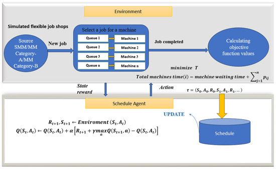
Figure 1.
Proposed QRL model for optimising the simulated job shops.
In the proposed QRL model, the learning rate (alpha) is 95%, the discount rate (gamma) is 0.1 and the max number of iterations is 10,000. The following is a discussion of the parameters in the proposed models of this study.
Alpha (α): The agent changes its Q-values depending on new experiences, which is determined by the learning rate represented by α. Regarding simulated FJSPs in this work, alpha affects how fast the agent modifies its scheduling decisions. When FJSPs are highly interactive, a more significant alpha can help because it speeds up learning. However, an excessively high learning rate t causes instability, and an excessively low learning rate can cause slow convergence.
Gamma (γ): The agent’s preference for immediate rewards over future rewards is determined by the discount factor, represented by the symbol γ. It impacts how the proposed RL models balance short- and long-term goals. Gamma is a critical component of the applied FJSPs, since it helps to balance the significance of quick scheduling decisions and their effects on long-term efficiency.
Greedy exploration (ε-Greedy): The ε-greedy exploration strategy combines exploitation and exploration. It entails choosing between a random action with the probability ε and the action with the highest Q-value (greedy action) with the probability 1 − ε. The ε-greedy approach in the applied FJSPs enables the agent to achieve a balance between the exploitation of proper strategies and the exploration of scheduling choices. More exploration is encouraged by a greater ε, which is advantageous in flexible scheduling environments. A smaller ε indicates more exploitation and the use of try-and-error methods.
5.3. Application of SARSA Model
The subsequent phase of this research entails developing a novel SARSA model. This model provides an on-policy approach because the state value is changed for each transition, and the revised state value affects the policy used to determine the behaviour. Algorithm 2 presents the standard SARSA algorithm [33,34]. Figure 2 shows the novel SARSA model for optimising job shops in this work. This model illustrates the initial environments used in the SARSA model, including 29 flexible job shops; the initial state begins to schedule the job sequences employing related rewards. The following are some features of this model.
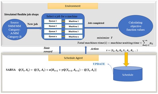
Figure 2.
Proposed SARSA model for optimising the simulated job shops.
- Agent: In this model, an agent interacts with the environment, gains knowledge and makes choices. When a job becomes available, it is selected from the local waiting queue of the machine (sometimes referred to as the job-candidate set) and processed. When the current operation is completed, each job chooses a machine to handle subsequent operations. At this point, the job becomes a job candidate for the machine and is assigned an agent for task routing; this is performed to address the vast action space of the FJSPs. Thus, the agent decides what is appropriate given the current state of the environment.
- States: The state represents the environment, including various machine and job-related aspects. Such aspects include the productivity of machines and how they interact with one another, the number of machines active and available for use in each operation and the workloads of the jobs completed or in progress at different operations; this aims to maximise returns or the sum of discounted rewards while minimising the makespan or the number of time steps required to accomplish the jobs.
- Reward: The rewards involve moving between jobs to calculate the makespan, which ultimately becomes an objective function. Regarding the state, the agent moves between jobs to calculate the time, add it to the reward, calculate the objective function and execution time for the entire benchmark (job shop), and cut down on time. By reversing the rewards, the minimum time in the program is calculated, wherein the agent increases the reward while the environment minimises the time.
| Algorithm 2. Standard SARSA |
| for all state-action pairs. For each episode, do |
| in the current episode, do |
| End for |
| End for |
The initial parameters of this model are as follows: the learning rate (alpha) is 1, the discount rate (gamma) is 0.09, the max number of iterations is 1000, and the greedy factor (Epsilon) is 0.9.
6. Results and Experimental Discussion
The results are compared with an advanced NMHPGA to examine the proposed models’ performance. SARSA performs better than different algorithms, indicating that it can solve the FJSP with satisfying solutions. The performance of the proposed RL’s convergence is shown in Figure 3 and Figure 4.
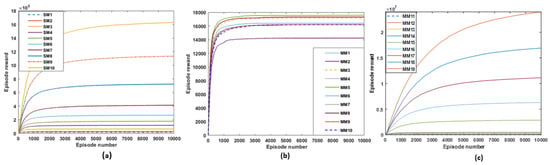
Figure 3.
Simulation results applying QRL model on SM category and MM Category-A and -B. (a) The rewards of applying QRL on SM1–SM10 to reach the best rewards. (b) The rewards of applying QRL on MM1–SM10 to reach the best rewards. (c) The rewards of applying QRL on MM11–MM19 to reach the best rewards.
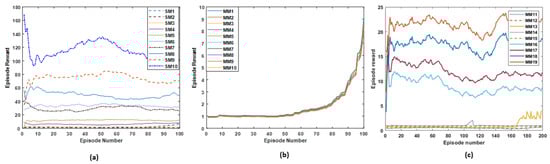
Figure 4.
Simulation results applying the proposed SARSA model on the SM category and MM Category-A and -B. (a) The rewards of applying the SARSA model on SM1–SM10 to reach the best rewards by increasing the episode numbers. (b) The rewards of applying the SARSA model on MM1–MM10 to reach the best rewards. (c) The rewards of applying the SARSA model on MM11–MM19 to reach the best rewards.
Table 3, Table 4 and Table 5 show the simulation results, comparing the objective functions for the RL-based Q-learning and SARSA models with NMHPGA. Each benchmark cell considerably improves the makespan. Table 3, Table 4 and Table 5 present the simulation results tested on SM (SM1–SM10), MM category-A (MM1–MM10) and MM category-B (MM11–MM19), respectively. It can be seen from the results that the Q-agent chooses the greedy action, which delivers the maximum Q-value for the state, and the proposed Q-learning algorithm performs poorly compared to the SARSA algorithm; however, when the size of the job shop Is large (MM11–MM19), the findings of this research show that the recommended Q-learning strategy outperforms the SARSA algorithm. Additionally, as shown in Table 4 and Table 5, by comparing the objective function values, it can be concluded that the GA technique outperforms the proposed Q-learning algorithm regarding apparent improvements for SM and MM job shops (because the objective function is lower than QRL results).
Table 3.
Comparison of the objective functions tested on job shops in the SM category.
Table 4.
Comparison of the objective functions tested on multi-machine job shops in Category-A.
Table 5.
Comparison of the objective functions tested on job shops in multi-machines Category B.
The statistical analysis of the objective functions in the SARSA algorithm and QRL are contrasted with those of NMHPGA. The performance differential relative to NMHPGA denotes the percentage improvement in the objective functions achieved by SARSA compared to NMHPGA. Furthermore, the QRL performance differential relative to NMHPGA (%) represents the percentage enhancement in the objective functions achieved by QRL compared to NMHPGA. The comparisons reveal that SARSA consistently demonstrates superior performance across all categories compared to the other models.
Results from QRL tested on the SM category and multi-machine Category-A and -B are shown in Figure 3. The simulation results for the SM categories SM1–SM10, comprising 10,000 iterations and maximum awards using QRL, are shown in Figure 3a. Figure 4a shows the outcomes of SM simulations using the SARSA model, which incorporates average rewards. As shown, by increasing the number of episodes, the agent learns from the environment to increase the reward. The results for MM job shops category-A using QRL and SARSA are shown in Figure 3b and Figure 4b, respectively. The simulation results show the average rewards, which increase over time, which means the agent increases the exploration and exploitation of the environment. Finally, Figure 3c shows the average rewards of each episode of applying QRL for job shop category-B. It is indicated that the agent tries exploring and exploitation to learn from the environment to reach the best reward.
7. Case Study: Reheating Furnace Model
This study optimises the furnace model schedule developed by [35]. The optimisation results from the proposed QRL and SARSA models are compared to the results of the NMHPGA. The optimisation aims to reduce the time and energy consumption in the furnace model. Although furnace designs may differ in terms of their intended use, such as within the heating processes, fuel type and techniques for introducing combustion air, most process furnaces have a few things in common [35]. The type of fuel, combustion efficiency, idle and cycling losses and heat transfer affect the furnace’s design and the heating schedule for the materials [35]. The project model needs to account for all the requirements, including the time and fuel used. The applied furnace model is a multi-objective function with three objectives: (1) reducing the time of the schedule, (2) reducing the furnace’s energy consumption, and (3) simultaneously reducing the time by 30% and energy by 70%. The latter is the most critical in terms of efficiency. Equations (7)–(9) show the above objectives in this model, where T is the time taken for each job, F is the fuel consumption per job, and n is the number of jobs.
Before optimisation, the furnace consumes 86.8673 × 10⁴ m3/h of fuel and takes 139.2167 h to operate. Equations (10) and (11) pertain to a dynamic model of the furnace temperature [35].
where
- : Time [min];
- : Dead time [min];
- : Total fuel flow rate in the heating furnace ;
- : The out-strip temperature ;
- : Non-negative integer;
- : Out-strip temperature ;
- : Strip temperature at the inlet of the furnace (constant) ;
- : Furnace temperature ;
- : Strip width and thickness ;
- : Line speed ;
- : Average line speed during is the heating time of the strip) [35].
The proposed RL models aim to reduce the time and energy needed in the furnace model. The environment in the following stage is the furnace model with three objectives: 1, 2, and 3. Each environment is run separately to obtain optimised results. The furnace model’s schedule is optimised by experimenting with various states and computing rewards; the best reward demonstrates the optimal sequence and schedule for the furnace model.
Table 6 shows the elapsed time results following schedule optimisation for the furnace model tested by the NMHPGA, QRL and SARSA. Table 7 shows the amount of energy used in this model. As presented in Table 7, the furnace uses 83.9666 × 10⁴ m3/h of fuel when NMHPGA is applied as an optimiser; in contrast, the SARSA model uses 84.1481 × 10⁴ m3/h. Despite these differences in fuel consumption, SARSA is highly recommended over complex GAs and Q-learning due to its simplicity and superior performance.
Table 6.
Comparison of the elapsed time (h) when applying NMHPGA, QRL and SARSA models on the furnace model.
Table 7.
Comparison of the fuel consumption when applying NMHPGA, QRL and SARSA methods on the furnace model.
The SARSA provides a similar schedule when using any objective, because SARSA finds optimal solutions despite other algorithms finding suboptimal solutions. Hence, there are no differences between the three objectives’ results for SARSA. NMHPGA and QRL, when executed, provide varying outcomes on each run due to their utilisation of random initial conditions.
Regarding furnace objectives, the optimal schedule involves achieving a balance between reducing both time and fuel consumption. Objectives 1 and 2 are still valid, as one optimises the time (urgent jobs), and the other optimises the energy. The operator can choose a schedule based on the customer’s requirements. Objective 3 is best for the company, saving both time and fuel. In summary, the proposed SARSA model finds a similar solution for any objective, which is the best solution, while QRL finds sub-optimal solutions.
As shown in Figure 5, the simulation results of the QRL agent on Objectives 1, 2 and 3 indicate that the agent increases the exploration–exploitation trade-off when the number of episodes increases. As a result, the agent learns from the environment and raises the reward at each state. There can be more episodes to reach more significant rewards; nevertheless, the maximum for QRL is 10,000. Similar average reward results when employing the SARSA model are shown in Figure 6a–c. The figures show that the graph fluctuation leads the agent’s learning rate to the best reward. The simulated furnace temperature findings are provided in Appendix A, which shows the temperature of the furnace over time.
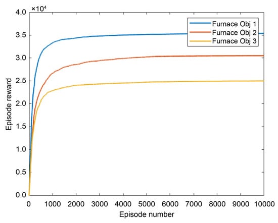
Figure 5.
QRL training model tested on furnace model (Objectives 1, 2 and 3). This figure compares the simulated rewards of applying QRL on three objectives of the furnace, including Objective 1, Objective 2 and Objective 3.
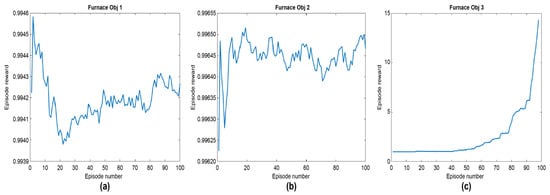
Figure 6.
SARSA training tested on the furnace model (Objectives 1, 2 and 3). (a) objective 1; (b) objective 2; (c) objective 3.
Figure 6a illustrates the average rewards of the SARSA model when applied to furnace Objective 1, revealing the fluctuations and changes in the rewards to reach the best reward. Figure 6b shows the average rewards of the SARSA model applied to furnace Objective 2, highlighting the fluctuations and changes in the rewards in order to reach the best reward and maximise performance. Figure 6c shows the average rewards of the SARSA model applied to the furnace Objective 3 to achieve the best reward.
8. Conclusions and Future Work
This study examined the performance of novel implementation of the RL-based SARSA and Q-learning algorithms to optimise the simulated job shops and schedules of a furnace model. In the proposed models, the RL learns how to link environmental states to the actions of an agent in order to optimise long-term rewards. An agent learns the optimal behaviour through trial-and-error interactions with the environment, which involves exploring various states to find the best action and, in turn, learning the optimal behaviour. The reward-based Q-learning updates the value for a state–action pair at each step, ensuring that the agent quickly approaches the ideal value. Consequently, the RL frequently generates superior results for JSSPs and FJSPs, compared to other stochastic methods. Based on the findings arising from the presented research, the following primary outcomes can be defined:
- Q-learning, a fundamental reinforcement learning model, outperforms the advanced GA (NMHPGA) because GA algorithms are more complex and time-consuming and require additional program functions.
- Most of the QRL results show the strong performance of the algorithm, except for a few job shops of more considerable sizes. The proposed SARSA model was used to enhance these results.
- Despite the poor performance of SARSA in scenarios involving large-scale job shops, it is still a highly recommended model because of its comparative simplicity compared to GAs; SARSA requires less execution time and involves fewer functions, which makes it a preferred option to run the program and optimise JSSPs.
- Additionally, the proposed SARSA outperformed the NMHPGA and QRL by optimising the furnace model using RL models. It can be concluded that the SARSA is sufficiently fast and accurate to optimise industrial production lines with moderate-sized schedules.
- Although some limitations and the outlined models’ difficulties preclude the complete application of RL in complex real production systems, ongoing research efforts could address these issues, resulting in improvements in the use of RL in industrial applications.
- Future DRL-based models and additional applicable benchmarks would be beneficial; this expansion can be achieved by integrating advanced optimisation techniques.
- Furthermore, as GA methods are predominantly characterised by their complexity and slow performance, integrating various RL models with advanced GA models may lead to significant performance improvement.
- As a final note in this paper, it is noticeable that RL approaches can address more complex problems, extending their applicability to encompass not only the multi-objective JSSPs but also the more demanding FJSPs.
Author Contributions
Conceptualization, M.A. and A.M.; methodology, M.A. and A.M.; software, M.A. and A.M.; writing—original draft preparation, A.M.; writing—review and editing, A.M. and M.A. All authors have read and agreed to the published version of the manuscript.
Funding
There is not funding for this research. The APC was funded by Brunel University London.
Data Availability Statement
The data that support the findings of this study are available from the corresponding author, M.A., upon reasonable request.
Conflicts of Interest
The authors declare no conflict of interest.
Appendix A
Figure A1 shows the temperature needed in the furnace model in the period of the schedules. The results for the simulated furnace temperature are shown in Figure A1, when applying QRL and SARSA. Figure A1a–c illustrates the QRL model results, and Figure A1d–f indicates the SARSA model results for the furnace model for Objectives 1, 2, and 3 (respectively).
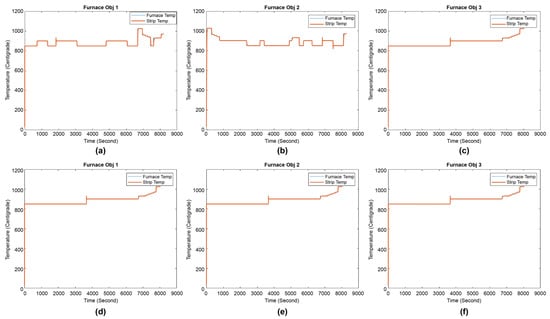
Figure A1.
Objective 1, 2 and 3 simulation results when using the QRL and SARSA models, showing the temperature needed. (a–c) illustrate the QRL results, testing Objectives 1 and 2. (d–f) indicate the results of the SARSA model tested on the furnace testing objectives 1, 2 and 3.
References
- Jamwal, A.; Agrawal, R.; Sharma, M.; Kumar, A.; Kumar, V.; Garza-Reyes, J.A.A. Machine Learning Applications for Sustainable Manufacturing: A Bibliometric-Based Review for Future Research. J. Enterp. Inf. Manag. 2022, 35, 566–596. [Google Scholar] [CrossRef]
- Machado, C.G.; Winroth, M.P.; Ribeiro da Silva, E.H.D. Sustainable Manufacturing in Industry 4.0: An Emerging Research Agenda. Int. J. Prod. Res. 2019, 58, 1462–1484. [Google Scholar] [CrossRef]
- Malek, J.; Desai, T.N. A Systematic Literature Review to Map Literature Focus of Sustainable Manufacturing. J. Clean. Prod. 2020, 256, 120345. [Google Scholar] [CrossRef]
- Pezzella, F.; Morganti, G.; Ciaschetti, G. A Genetic Algorithm for the Flexible Job-Shop Scheduling Problem. Comput. Oper. Res. 2008, 35, 3202–3212. [Google Scholar] [CrossRef]
- Liu, Z.; Guo, S.; Wang, L. Integrated Green Scheduling Optimization of Flexible Job Shop and Crane Transportation Considering Comprehensive Energy Consumption. J. Clean. Prod. 2019, 211, 765–786. [Google Scholar] [CrossRef]
- Yuan, Y.; Xu, H. Multi-objective Flexible Job Shop Scheduling Using Memetic Algorithms. IEEE Trans. Autom. Sci. Eng. 2015, 12, 336–353. [Google Scholar] [CrossRef]
- Park, I.B.; Huh, J.; Kim, J.; Park, J. A Reinforcement Learning Approach to Robust Scheduling of Semiconductor Manufacturing Facilities. IEEE Trans. Autom. Sci. Eng. 2020, 17, 1420–1431. [Google Scholar] [CrossRef]
- Gao, K.; Cao, Z.; Zhang, L.; Chen, Z.; Han, Y.; Pan, Q. A Review on Swarm Intelligence and Evolutionary Algorithms for Solving Flexible Job Shop Scheduling Problems. IEEE/CAA J. Autom. Sin. 2019, 6, 904–916. [Google Scholar] [CrossRef]
- Momenikorbekandi, A.; Abbod, M. A Novel Metaheuristic Hybrid Parthenogenetic Algorithm for Job Shop Scheduling Problems: Applying Optimisation Model. IEEE Access 2023, 11, 56027–56045. [Google Scholar] [CrossRef]
- Brucker, P.; Schlie, R. Job-Shop Scheduling with Multi-Purpose Machines. Computing 1990, 45, 369–375. [Google Scholar] [CrossRef]
- Brandimarte, P. Routing and Scheduling in a Flexible Job Shop by Tabu Search. Ann. Oper. Res. 1993, 41, 157–183. [Google Scholar] [CrossRef]
- Jiang, E.d.; Wang, L. Multi-Objective Optimization Based on Decomposition for Flexible Job Shop Scheduling under Time-of-Use Electricity Prices. Knowl. Based Syst. 2020, 204, 106177. [Google Scholar] [CrossRef]
- Li, Y.; Huang, W.; Wu, R.; Guo, K. An Improved Artificial Bee Colony Algorithm for Solving Multi-Objective Low-Carbon Flexible Job Shop Scheduling Problem. Appl. Soft Comput. 2020, 95, 106544. [Google Scholar] [CrossRef]
- Li, J.Q.; Song, M.X.; Wang, L.; Duan, P.Y.; Han, Y.Y.; Sang, H.Y.; Pan, Q.K. Hybrid Artificial Bee Colony Algorithm for a Parallel Batching Distributed Flow-Shop Problem with Deteriorating Jobs. IEEE Trans. Cybern. 2020, 50, 2425–2439. [Google Scholar] [CrossRef] [PubMed]
- Mahmoodjanloo, M.; Tavakkoli-Moghaddam, R.; Baboli, A.; Bozorgi-Amiri, A. Flexible Job Shop Scheduling Problem with Reconfigurable Machine Tools: An Improved Differential Evolution Algorithm. Appl. Soft Comput. 2020, 94, 106416. [Google Scholar] [CrossRef]
- Zhang, S.; Li, X.; Zhang, B.; Wang, S. Multi-Objective Optimisation in Flexible Assembly Job Shop Scheduling Using a Distributed Ant Colony System. Eur. J. Oper. Res. 2020, 283, 441–460. [Google Scholar] [CrossRef]
- Yang, Y.; Huang, M.; Yu Wang, Z.; Bing Zhu, Q. Robust Scheduling Based on Extreme Learning Machine for Bi-Objective Flexible Job-Shop Problems with Machine Breakdowns. Expert Syst. Appl. 2020, 158, 113545. [Google Scholar] [CrossRef]
- Zhang, G.; Shao, X.; Li, P.; Gao, L. An Effective Hybrid Particle Swarm Optimisation Algorithm for Multi-Objective Flexible Job-Shop Scheduling Problem. Comput. Ind. Eng. 2009, 56, 1309–1318. [Google Scholar] [CrossRef]
- Mihoubi, B.; Bouzouia, B.; Gaham, M. Reactive Scheduling Approach for Solving a Realistic Flexible Job Shop Scheduling Problem. Int. J. Prod. Res. 2021, 59, 5790–5808. [Google Scholar] [CrossRef]
- Wu, X.; Peng, J.; Xiao, X.; Wu, S. An Effective Approach for the Dual-Resource Flexible Job Shop Scheduling Problem Considering Loading and Unloading. J. Intell. Manuf. 2021, 32, 707–728. [Google Scholar] [CrossRef]
- Momenikorbekandi, A.; Abbod, M.F. Multi-Ethnicity Genetic Algorithm for Job Shop Scheduling Problems. 2021. Available online: https://ijssst.info/Vol-22/No-1/paper13.pdf (accessed on 16 November 2023).
- Bellman, R. A Markovian Decision Process. Indiana Univ. Math. J. 1957, 6, 679–684. [Google Scholar] [CrossRef]
- Oliff, H.; Liu, Y.; Kumar, M.; Williams, M.; Ryan, M. Reinforcement Learning for Facilitating Human-Robot-Interaction in Manufacturing. J. Manuf. Syst. 2020, 56, 326–340. [Google Scholar] [CrossRef]
- Watkins, C.J.C.H.; Dayan, P. Q-Learning. Mach. Learn. 1992, 8, 279–292. [Google Scholar] [CrossRef]
- Shahrabi, J.; Adibi, M.A.; Mahootchi, M. A Reinforcement Learning Approach to Parameter Estimation in Dynamic Job Shop Scheduling. Comput. Ind. Eng. 2017, 110, 75–82. [Google Scholar] [CrossRef]
- Shen, X.N.; Minku, L.L.; Marturi, N.; Guo, Y.N.; Han, Y. A Q-Learning-Based Memetic Algorithm for Multi-Objective Dynamic Software Project Scheduling. Inf. Sci. 2018, 428, 1–29. [Google Scholar] [CrossRef]
- Lin, C.C.; Deng, D.J.; Chih, Y.L.; Chiu, H.T. Smart Manufacturing Scheduling with Edge Computing Using Multiclass Deep Q Network. IEEE Trans. Industr. Inform. 2019, 15, 4276–4284. [Google Scholar] [CrossRef]
- Shi, D.; Fan, W.; Xiao, Y.; Lin, T.; Xing, C. Intelligent Scheduling of Discrete Automated Production Line via Deep Reinforcement Learning. Int. J. Prod. Res. 2020, 58, 3362–3380. [Google Scholar] [CrossRef]
- Luo, S. Dynamic Scheduling for Flexible Job Shop with New Job Insertions by Deep Reinforcement Learning. Appl. Soft Comput. 2020, 91, 106208. [Google Scholar] [CrossRef]
- Chen, R.; Yang, B.; Li, S.; Wang, S. A Self-Learning Genetic Algorithm Based on Reinforcement Learning for Flexible Job-Shop Scheduling Problem. Comput. Ind. Eng. 2020, 149, 106778. [Google Scholar] [CrossRef]
- Panzer, M.; Bender, B. Deep Reinforcement Learning in Production Systems: A Systematic Literature Review. Int. J. Prod. Res. 2021, 60, 4316–4341. [Google Scholar] [CrossRef]
- Sivanandam, S.N.; Deepa, S.N. Genetic Algorithms. In Introduction to Genetic Algorithms; Springer: Berlin/Heidelberg, Germany, 2008; pp. 15–37. [Google Scholar] [CrossRef]
- Dong, H.; Ding, Z.; Zhang, S. Deep Reinforcement Learning: Fundamentals, Research and Applications; Springer: Singapore, 2020; pp. 1–514. [Google Scholar] [CrossRef]
- Sewak, M. Policy-Based Reinforcement Learning Approaches: Stochastic Policy Gradient and the REINFORCE Algorithm. In Deep Reinforcement Learning; Springer: Singapore, 2019; pp. 127–140. [Google Scholar] [CrossRef]
- Yoshitani, N.; Hasegawa, A. Model-Based Control of Strip Temperature for the Heating Furnace in Continuous Annealing. IEEE Trans. Control Syst. Technol. 1998, 6, 146–156. [Google Scholar] [CrossRef]
Disclaimer/Publisher’s Note: The statements, opinions and data contained in all publications are solely those of the individual author(s) and contributor(s) and not of MDPI and/or the editor(s). MDPI and/or the editor(s) disclaim responsibility for any injury to people or property resulting from any ideas, methods, instructions or products referred to in the content. |
© 2023 by the authors. Licensee MDPI, Basel, Switzerland. This article is an open access article distributed under the terms and conditions of the Creative Commons Attribution (CC BY) license (https://creativecommons.org/licenses/by/4.0/).