Prediction of the Deformation of Heritage Building Communities under the Integration of Attention Mechanisms and SBAS Technology

Abstract

The protection of heritage building communities is of important historical significance, the occurrence of a landslide is related to the safety and stability of the heritage building, and ground monitoring and forecasting are the key steps for the early warning and timely restoration of the heritage building. This study utilizes remote sensing technology to monitor the ground of a cultural heritage building, and employs a Long Short-Term Memory (LSTM) network for prediction. Firstly, we conducted ground subsidence monitoring within a specific time series of the study area using heritage remote sensing images and SBAS-InSAR technology. Following the subsidence monitoring, and incorporating an attention mechanism, we effectively localized and extracted features of heritage building clusters within the region. This approach efficiently addresses the challenge of feature identification resulting from the dense distribution of buildings and the similarity between various objects. The results indicate that the maximum subsidence rate in the research area reached −60 mm/year, reached a maximum uplift rate of 45 mm/year, and that the maximum cumulative subsidence reached −65 mm. Secondly, for the multi-level, multi-scale, and class-specific objects in remote sensing images, the LSTM network enables adaptive contextual information during deep and shallow feature extraction. This allows for better contextual modeling and the correlation between predicted and actual results reaches a 0.95 correlation, demonstrating the accurate predictive performance of the LSTM network. In conclusion, both LSTM and SBAS technologies play a crucial role in decision-making for heritage buildings, facilitating effective early warning and disaster mitigation.

1. Introduction

Natural disasters possess distinctive traits characterized by their high destructiveness and abrupt occurrence. These attributes render them challenging to preempt, thus imposing a substantial threat to heritage buildings. Ground subsidence resulting from natural disasters proves exceedingly detrimental to the stability of heritage structures. Cumulative ground subsidence can readily give rise to a myriad of perils, including structural and infrastructural damage, as well as impeding subterranean engineering, all of which severely compromise the safety of people and property, leading to economic losses. Heritage buildings constitute a pivotal component of a nation’s or region’s cultural and historical legacy, boasting irreplaceable historical and cultural significance. However, the morphology and structural integrity of heritage structures can undergo transformation due to the influence of both natural disasters and human activities, potentially undermining their cultural and historical value. Recent years have witnessed numerous instances of building damage attributable to the impact of natural disasters. In recent years, there have been countless cases of building damage caused by natural disasters. Recently, more than 100 immovable cultural relics in the south of a certain place have been damaged due to natural disasters, and more than 10,000 immovable cultural relics have been damaged due to natural disasters. Among these damaged cultural relics are not only ancient buildings, temples, palaces, and other buildings, but also the collapse of ancient city walls. At present, over 50 cities in China have experienced varying degrees of land subsidence. Therefore, the issue of land subsidence has become an important geological issue of global concern. In the face of the problem of land subsidence of heritage buildings, it is urgent to monitor, analyze, and predict the spatiotemporal changes in land subsidence in order to take effective protection measures in a timely manner.

In recent years, there has been extensive research into heritage building monitoring methods using remote sensing technology. However, traditional surveillance approaches have exhibited certain issues, such as higher error rates and limited monitoring accuracy. With the advancement of digital mapping and remote sensing technology, the monitoring of architectural heritage has become more streamlined and accessible. Several regions within the country have also initiated heritage monitoring efforts. Nevertheless, these initiatives often rely on techniques like 3D laser scanning, digital photography measurement, and drone technology for capturing architectural structures, with comparatively less emphasis on the detailed analysis of building shapes and surfaces. Therefore, this paper will use the emerging Interferometric Synthetic Aperture Radar technology (InSAR). It aims to detect the risk of deformation of heritage buildings in a particular region of the country [1]. InSAR technology is a set of interferences and measurements as a single remote sensing technology, for urban ground sediment monitoring; the most widely applied of these are timescale InSAR technologies, such as permanent scatterer synthetic aperture radar interferometry (PS-InSAR) and Small Baseline Subset InSAR (SBAS-InSAR) [2]. These set reasonable time and spatial base thresholds, combine different SAR images into several interference pairs, and then calculate the corresponding surface sedimentation value for each intervention, so as to obtain the time of execution of the study area. The urban precipitation phenomenon is due to many factors, its subsurface precipitation generally shows irregularity, and there is no unified forecast model. Most of the study is also focused on how to improve the monitoring accuracy of urban surface variation due to the lack of reasonable forecasting of building variables and trends, so it is not possible to provide a predictive analysis of the target location of the building or the size of the regional long-term variable [3]. So, how to apply the timeline-based InSAR technology to build a method that can effectively predict urban surface transformation is the focus of the current research. In the field of surface deformation monitoring, compared with the traditional surface deformation monitoring technology in the level meter measurement, GNSS measurements, full stationary measuring, and other technologies, there is small scope in terms of coverage, low work efficiency, high cost, and difficulty in quantifying the large scope and other restrictions. InSAR technology has a high accuracy, broad scope, is not influenced by weather characteristics, and can effectively break through the above problems; therefore, it is widely used by scholars to monitor the ground, buildings, and other infrastructures. To better understand the deformation of a heritage building, we have used the Small Baseline Set (SBAS) technology to monitor the architectural heritage in order to obtain the timing of the heritage building for analysis and management. In order to better observe the deformation and development of architectural heritage, this paper uses the SBAS monitoring results as a data source to use deep learning [4,5,6] to predict the future deformations to improve the accuracy and reliability of the monitoring of heritage buildings. Soil precipitation, also referred to as surface subsidence or land subsidence, is a geological phenomenon resulting from the gradual settling of the Earth’s surface in localized areas. Changes in the Earth’s surface can lead to varying degrees of geological disasters. Land subsidence is primarily caused by two factors. On the one hand, there are natural factors, including the degradation of geological structures, earthquakes, volcanic eruptions, climate change, changes in the earth’s natural stress structure, and the natural solidity of the geological soil. On the other hand, there are factors including resources mining, the excavation and comprehensive use of groundwater, natural gas, oil, and other resources, urban infrastructure construction, and other artificial factors [7]. In recent years, due to the rapid development of the economy, the level of urbanization continues to improve, the various infrastructures on the surface of the ground have gradually improved, all kinds of large-scale projects and buildings have been created, and the areas affected by landslide disasters have also been expanded from local coastal cities to surrounding inland cities. Some areas have accumulated landslides of more than 150 mm, and surface cracks caused by uneven landsliding have even appeared. From this, it can be known that the surface sedimentation has a close relationship with the development of the regional economy, so the monitoring of the evolution of the urban surface is necessary, and the establishment of an effective monitoring and forecasting system is important for the protection of the people’s safety and of production and life in the precipitation zone.

In this study, we harnessed SBAS technology to extract deformation data pertaining to architectural heritage. To address spatial and temporal challenges more effectively, we employed LSTM models for predictive analysis in our research areas. Additionally, we incorporated attention mechanisms to capture distinctive architectural features across regions. Traditional methods for predicting construction settlement often treat all regions’ characteristics equally, overlooking variations among different areas. By introducing attention mechanisms, we assign varying weights based on each region’s unique attributes, enabling a more precise delineation of specific area features. This paper integrates remote sensing technology into heritage building monitoring, taking full advantage of remote sensing’s benefits, including cost-efficiency, resource conservation, and non-contact capability. This approach enables the swifter tracking of architectural heritage’s evolution trends.

Among them, the contribution points of this article can be summarized in the following three aspects:

(1)

With SBAS-InSAR technology, it is possible to effectively process interference data from multiple time phases, thereby obtaining high-precision surface deformation information, effectively reducing nonlinear deformations on the Earth’s surface, such as terrain, land use changes, etc., making the deforming signals more obvious. By adopting multiple small base line combinations, large range values and more phase measurements can be obtained, thus improving the accuracy of deformed measurement and effectively handling SAR data under different seasonal and weather conditions, so as to obtain more accurate formation information.

(2)

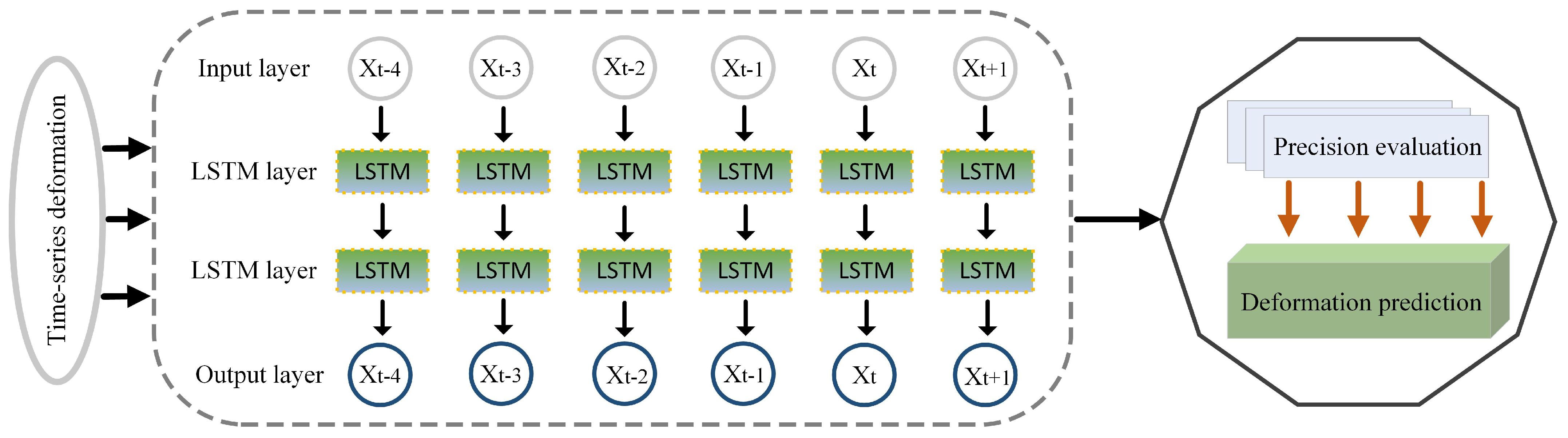
By leveraging LSTM’s capabilities in adaptive receptive fields, context modeling, and multi-level, multi-scale feature extraction, predictive models in remote sensing image analysis can more accurately capture crucial information within the data, thereby enhancing the quality and reliability of prediction outcomes.

(3)

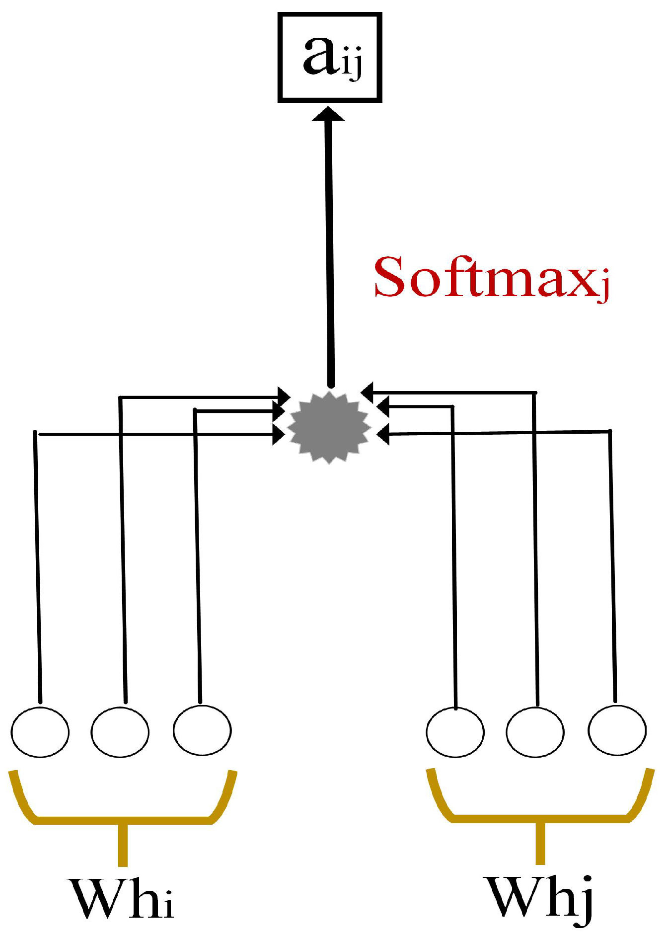
By incorporating an attention mechanism, the model can adaptively select features and weigh them, enhancing the model’s perception of crucial information within the data. This not only improves the accuracy of predicting deformations in architectural clusters but also increases the interpretability of the model.

The logical structure of this article is as follows:

In Section 2, we presented the relevant work, approximately describing the research methods we have proposed, primarily exploring and discussing methods for predicting surface architectural formations; in Section 3, we introduced the main methods of this article, such as SBAS technology, LSTM, and attention mechanisms, etc.; in Section 4, we discussed the experimental parts, conducted comparative experiments, and demonstrated them; in Section 5, we introduce the discussion section, outlining the methodological thinking in this article and recent methodological discussions, as well as outlining the shortcomings of this methodology; and, in Section 6, we presented a final summary of the conclusions, summarized the methodology, and discussed the prospects for future work.

2. Related Work

In modern society, the protection and management of heritage buildings has long been an important topic, and forecasting the shapes of the heritage building communities has also become a hot spot for research. This article proposes a new approach to technology integration, namely the SBAS technology convergence attention mechanism, to predict the deformation of heritage building communities. Prior to this study, many scholars have explored and studied the monitoring of formations in heritage building communities, some of which mainly use traditional formation monitoring methods, such as full stationers, GPS, InSAR, and so on. For example, the authors of reference [8] achieved a better effect with the use of the full-stage monitoring of an ancient building; and reference [9] uses InSAR technology to monitor the massive heritage building communities, and obtains more accurate information about the transformation. However, these approaches have problems with monitoring accuracy that are greatly influenced by environmental conditions and human factors, and require a lot of human and material resources, making large-scale remote sensing monitoring difficult. For example, reference [10] proposes a formation monitoring method based on remote sensing images, which uses bilateral filters to suppress noise, and then uses the pixel deviation algorithm to monitor formation to obtain more accurate formation information. Reference [11] uses the CNN to process remote sensor images, and combines timing differentiation to monitor the formation to obtain more precise results.

InSAR technology was developed by the ground radar system, which is a fusion of synthetic porous radar remote sensing imaging and electromagnetic wave interference technology. With the continuous depth of scientific and technological research in countries around the world, coupled with the impact of Yang’s double-sewing interference experiment, in the late 1960s, improved intervention technology was introduced, through the joint intervention processing of two SAR images from different periods in the same region, from which the corresponding pixel intervention phase signal was extracted. Thus, the establishment of DEM in the region to three-dimensional surface visualization [12] was achieved, forming the relevant concept of InSAR [13]. InSAR technology has begun to gain traction and has achieved greater development. Since then, more and more scientists have also been committed to the development of InSAR, addressing its shortcomings and continuously offering new insights and methods to promote the gradual maturity of InSAR technology. Reference [14] achieved high-precision surface deformation monitoring through InSAR technology, which has been widely applied in tectonic geology, seismic research, and environmental change monitoring such as subsidence and uplift. However, the coherence is limited, requiring the monitoring area’s features to have certain radiation and reflection characteristics. Therefore, there may be difficulties in obtaining data in areas with forest cover and dense urban high-rise buildings. Reference [15] proved the ability to work under any weather and lighting conditions through SAR, so InSAR technology is not limited by time and weather, and is suitable for monitoring on a global scale. However, the error sources of InSAR technology involve multiple factors, such as the atmosphere and ionosphere, and precise data processing and correction are required to obtain accurate deformation information. The authors of reference [16] obtained surface deformation information using InSAR technology at multiple time phases, providing monitoring capabilities in time series, which helps in understanding the trend and periodicity of surface changes. However, in complex terrain or densely populated areas with high buildings, the obstruction of ground objects may lead to a decrease in InSAR data resolution, affecting the accuracy of monitoring. Reference [17] utilizes InSAR technology to obtain three-dimensional deformation information in the directions of surface subsidence and uplift, providing strong support for geological disaster warning and land resource management. However, data processing and analysis also require a large amount of computational resources and professional knowledge, resulting in high costs. To surmount this challenge, some researchers have introduced PS-InSAR technology and conducted both theoretical and experimental investigations. This technology was applied to an experiment involving 41 ERS SAR images covering Pomona City, California, in the United States. The experimental outcomes underwent processing via interpolation methods, yielding the ground deformation field within the study area. This established a foundational application for PS-InSAR technology in surface deformation monitoring. In subsequent years, researchers introduced SBAS-InSAR and Time Series InSAR monitoring technologies. These two ground monitoring methods effectively mitigate the limitations of D-InSAR technology, delivering monitoring results with millimeter-level precision. They address issues related to spatiotemporal decorrelation and atmospheric delay errors resulting from extensive spatiotemporal baselines. By further integrating temporal InSAR technology with predictive models, it becomes possible to achieve the large-scale monitoring and prediction of land subsidence. The predictive outcomes can offer valuable regional disaster prevention and control guidance, effectively averting disasters stemming from land subsidence. In order to detect surface deformation in vegetation-covered areas, some researchers have proposed the method of spatiotemporal correlation analysis using interferograms, which successfully detected surface deformation in vegetation areas [18]. This method breaks the claim that InSAR technology is not applicable to vegetation areas and has significant significance for the development of InSAR technology.

There are research scholars using different intelligent algorithms combined with probability punctuation methods to establish predicted parameter replay models separately, and counter performance predictive parameters, which are successful practices in the forecast of mobile deformation in mines. But, in combination with InSAR data forecasts, the three-dimensional formation of the surface of mines means that the current research results are not rich. Reference [19] proposes a method for predicting three-dimensional surface deformation in mining areas based on probability integral models and monorail InSAR data. This method has greatly promoted the research progress of surface deformation prediction in InSAR mining areas, but there are still limitations. Therefore, some researchers have directly converted LOS deformation to vertical deformation, using the results of vertical deformation as the data source to estimate the expected parameters of subsidence using the probability integration method, while the horizontal movement coefficient refers to empirical values, which cannot fully obtain all expected parameters. Reference [20] proposed PS free networking, the calculation of separation information, the PS timing analysis method being brought into the atmosphere correction, and promoted the theoretical research and application of PS-InSAR technology. In recent years, the application of PS- InSAR technology has made unprecedented progress, especially in surface deformation monitoring. Researchers have used PS-InSAR technology to process 35 Sentinel-1A images of a certain region from 2018 to 2020. Based on the average annual deformation rate and cumulative deformation variables obtained from three subway lines, the spatiotemporal characteristics of surface deformation in the region are analyzed, and a conclusion is drawn that there is a positive correlation between groundwater level change information and surface deformation information. Finally, a summary is established regarding the interrelationship between the spatiotemporal characteristics of surface deformation in the region and its influencing factors. Reference [21] uses 44 COSMO SkyMed Satellite imagery as the data source, and uses PS-InSAR technology to obtain the surface deformation information of a built-up area of a city from 2013 to 2016. Combining the engineering construction data and the actual survey data, it analyzes the reasons for the surface deformation, and finally summarizes the spatio-temporal characteristics of the surface deformation of the built-up area of the city. Reference [22] is based on Sentinel-1A images covering a certain area, using the StaMPS method and interferogram superposition method to obtain the surface deformation process of the area from May 2017 to December 2018. Combined with local groundwater level information, it reveals the reasons for the coal mine collapse area.

With regard to the limitations of the above method, researchers have used InSAR’s spatial geometry as a theoretical basis, reconstructing the surface shapes so as to obtain a three-dimensional variation in the vertical, east, and south–north directions. Then, they combine the probability pointing method and INSAR technology, thereby building a functional model of both, using intelligent algorithms to collect all the expected parameters, and using the probability pointing method for subsequent mining for prediction. Subsequently, research on InSAR’s forecast of the three-dimensional deformation of the surface of the mine was gradually enriched [23]. Researchers have once again proposed the Boltzmann function forecast model, which is more suitable for D-InSAR monitoring properties, and combined the model with InSAR data to establish a system of three-dimensional surface formation forecasts suited to different levels of capture. In addition, reference [24] fused InSAR data and GA to construct an inversion model for predicting mining subsidence parameters, and obtained the dynamic probability integral prediction parameters for mining subsidence in the mining area. With the emergence of deep learning, various neural network prediction models [25] have been applied in the field of Deformation monitoring. By using deep learning prediction models, we analyze the temporal evolution and characteristics of surface subsidence, and accurately predict the subsidence situation in the study area.

3. Method

The overall algorithm flowchart of this article is shown in Figure 1; the proposed framework comprises three key modules. The first module is dedicated to deformation monitoring and analysis. It processes multiple time-phase SAR images obtained from remote sensing equipment. SBAS InSAR technology is employed to calculate surface deformation by comparing SAR interferograms at various time points. This yields highly precise surface deformation information. The processed deformation data, including accuracy calculations and other relevant metrics, are scrutinized to assess the processing quality at this stage. The second module involves model training. Using the surface deformation data obtained in the first module, a time series is constructed to visualize the surface deformation’s evolution over time. The time series data are divided into training and test sets for model training and verification. An LSTM network structure is employed to predict surface deformation. The LSTM exhibits excellent memory capabilities when handling time series data. The introduction of an attention mechanism empowers the model to adaptively select and weigh deformation information from different time points, thereby enhancing the capture of dynamic deformation characteristics. Appropriate loss functions are used to calculate the discrepancy between predicted and actual values, facilitating model performance evaluation during training. Subsequently, based on the loss value, a backpropagation algorithm calculates the gradient, and optimization techniques like gradient descent are utilized to update model parameters, continually enhancing the model’s predictive capabilities. The third module utilizes the trained LSTM model to predict point-to-point deformation in new time series data, allowing for the estimation of future surface deformation trends. The precision and accuracy of the model are evaluated based on the model’s predictive results through error calculations and other assessment metrics. Subsequently, surface deformation prediction results are obtained, which can be applied in tasks such as surface deformation monitoring and disaster forecasting. Through the seamless integration of these three modules, the proposed algorithm comprehensively leverages SBAS InSAR technology, LSTM neural networks, and attention mechanisms to achieve high-precision surface deformation prediction and monitoring. This approach provides effective tools for safeguarding and disaster prevention within heritage building communities.

3.1. SBAS Technology

SBAS technology is a method for InSAR time series analysis that is based on multiple master images. It extracts surface deformation information by using only interferograms with short temporal and spatial baselines. In a study by the authors of reference [26], this technique was used to monitor the deformation of a circular mountain in southern Italy, demonstrating its effectiveness. During the data processing, this method combines the data appropriately to generate short baseline differenced interferograms [27], which helps overcome the issue of spatial decorrelation. To estimate the deformation rates, Singular Value Decomposition (SVD) can be used to connect isolated SAR datasets generated from large baselines, thereby improving the sampling rate of the observed data. The time series analysis of Synthetic Aperture Radar (SAR) images involves the synthesis of SAR images from different data sources or different maps of the same source. The specific procedure is as follows: first, a common master image is chosen from the SAR images that cover the same area. Then, the other images are registered to the master image to generate interferograms, and the coherence coefficient, ${\omega }_{i,j}$, of the interferograms is calculated using the following formula:

$${\omega }_{i,j}=\left(1-f\left(\frac{T^{i,j}}{T^t}\right)\right)·\left(1-f\left(\frac{B^{i,j}}{B^t}\right)\right)·\left(1-f\left(\frac{D^{i,j}}{D^t}\right)\right)$$

(1)

$$f\left(x\right)=\left\{\begin{array}{cc}x,\hfill & x\le 1\hfill \\ 1,\hfill & x>1\hfill \end{array}\right.$$

(2)

In the given equation, $T^t$, $B^t$, and $D^t$ represent the thresholds for time baseline, spatial vertical baseline, and Doppler centroid frequency, respectively. By calculating the coherence coefficient ${\omega }_{i,j}$ between every pair of images, we obtain a coefficient matrix. We then sum up each row of the matrix.

$${\omega }_i=\frac{1}{N-1}\sum _{j=1,j\ne i}^N{\omega }_{i,j}$$

(3)

Among them, N is the number of images, calculated as the corresponding coefficient ${\omega }_i$ of the first i image of the public image, and we compared the image at the maximum value ${\omega }_i$. At this point, the selected common reference image achieves the optimal combination of time baseline, spatial perpendicular baseline, and Doppler centroid frequency baseline. Once the common reference image is chosen, all the images are registered and resampled to match the reference image. When two interferometric SAR images are accurately registered, the interferometric fringes appear in their interferogram. InSAR processing extracts ground elevation and deformation information by analyzing the interferogram. Therefore, image registration is a critical step in time-series InSAR processing. The specific registration steps are as follows.

Assuming we have two SAR complex images, $P_1(x,y)$ and $P_2(x,y)$, the calculation formula for the interferogram is as follows, when there is an integer pixel offset between the two images.

$$I(x,y;m,n)=P_1^{\ast }(x,y)·P_2(x-m,y-n)$$

(4)

where $(m,n)$ represents the pixel offset of an integer and represents conjugation. In image registration, the expression of SNR is as follows:

$$SNR(m,n)=\frac{{max}_{\begin{array}{c}0\le k<M<M\\ 0\le l<N\end{array}}|\tilde{I}(k,l;m,n)|}{{\sum }_{k=0}^{M-1}{\sum }_{l=0}^{N-1}|\tilde{I}(k,l;m,n)|-{max}_{\begin{array}{c}0\le k<M\\ 0\le l<N\end{array}}|\tilde{I}(k,l;m,n)|}$$

(5)

where $\tilde{I}\left(k,l;m,n\right)$ is the spectrum of the interferogram, which can be obtained using the following formula:

$$\tilde{I}(k,l;m,n)=\frac{1}{MN}\sum _{x=1}^M\sum _{y=1}^{N}I(x,y;m,n)·exp\left[-j2\pi \left(\frac{kx}{M}+\frac{ly}{N}\right)\right]$$

(6)

In the given equation, M and N represent the number of rows and columns in the interferogram spectrum. When two images are precisely registered, their signal-to-noise ratio (SNR) reaches its maximum value. Therefore, to determine the offset between the interference relative values, we iterate through all possible offset positions and identify the position with the maximum SNR and its corresponding offset. We set predefined time baseline and spatial baseline thresholds and generate some interference pairs with better interference conditions based on the set thresholds, thus eliminating interference pairs with poorer interference conditions. The Goldstein method is used for filtering, and the minimum cost flow method is used for unwrapping. In the interferometric dataset of the time series, the interference phase in any scene interference image is represented as follows:

$${\varphi }_{int}={\varphi }_{atmos}+{\varphi }_{topo}+{\varphi }_{defo}+{\varphi }_{object}+{\varphi }_{orbit}+{\varphi }_{noise}$$

(7)

After subtracting the elevation phase, the differential interference phase is obtained.

$$\begin{array}{c}{\phi }_{-}\mathrm{diff}={\phi }_{\_}atmos+{\phi }_{-}\left(topo\_error\right)+{\phi }_{-}defo+{\phi }_{-}\mathrm{object}+\hfill \\ {\phi }_{\_}\mathrm{orbit}+{\phi }_{-}\mathrm{noise}\hfill \end{array}$$

(8)

The interferometric phase values of the pixels in azimuth coordinate a and range coordinate i for the jth scene differential interferogram are expressed as follows:

$$\begin{array}{cc}\hfill \delta {\phi }_j(a,r)=& \frac{4\pi }{\lambda }\left[d\left(t_B,a,r\right)-d\left(t_A,a,r\right)\right]+\Delta {\varphi }_{\mathrm{topo}}^j(a,r)\hfill \\ \hfill & +\Delta {\varphi }_{aps}^j\left(t_B,t_A,a,r\right)+\Delta {\varphi }_{\mathrm{noise}}^j(a,r)\hfill \end{array}$$

(9)

In the formula, j represents the number of images, ranging from $(1,\dots ,N)$. It represents the central wavelength of the scene signal and the cumulative shape variables $d(t_B,a,r)$ and $d(t_A,a,r)$ of radar line of sight A and B. $topoj(a,r)$ represents the residual terrain phase in the differential interferogram, $apsj(tB,tA,a,r)$ represents the atmospheric phase, and $noisej(a,r)$ represents the total noise component of the model. In addition to using the minimum cost flow, Delaunay triangulation is also used to integrate the unwrapped results of several blocks into the overall optrimization, further improving the stability of the results. The atmospheric phase and residuals are removed by extracting robust and reliable stable points from the time series SAR data, and ground target points are extracted using the following methods:

(1)

Extracting high coherence points in a time series. The average interferogram in the SBAS method is used to select high coherence points in the time series, and the set short temporal and spatial baselines are used to ensure the quantity of coherence points.

(2)

After extracting high coherence points from the time series, I will select the high coherence points from the extracted time series that are located at the same positions in two or more sets of different source interference images.

(3)

The selected reference point should be a stable and passive interferogram, and its backscatter characteristics should be similar to the SAR data from different sources. To address the potential occurrence of large-scale incoherent and coherent deviations in the interferogram, set the coherence threshold to be greater than 0.18.

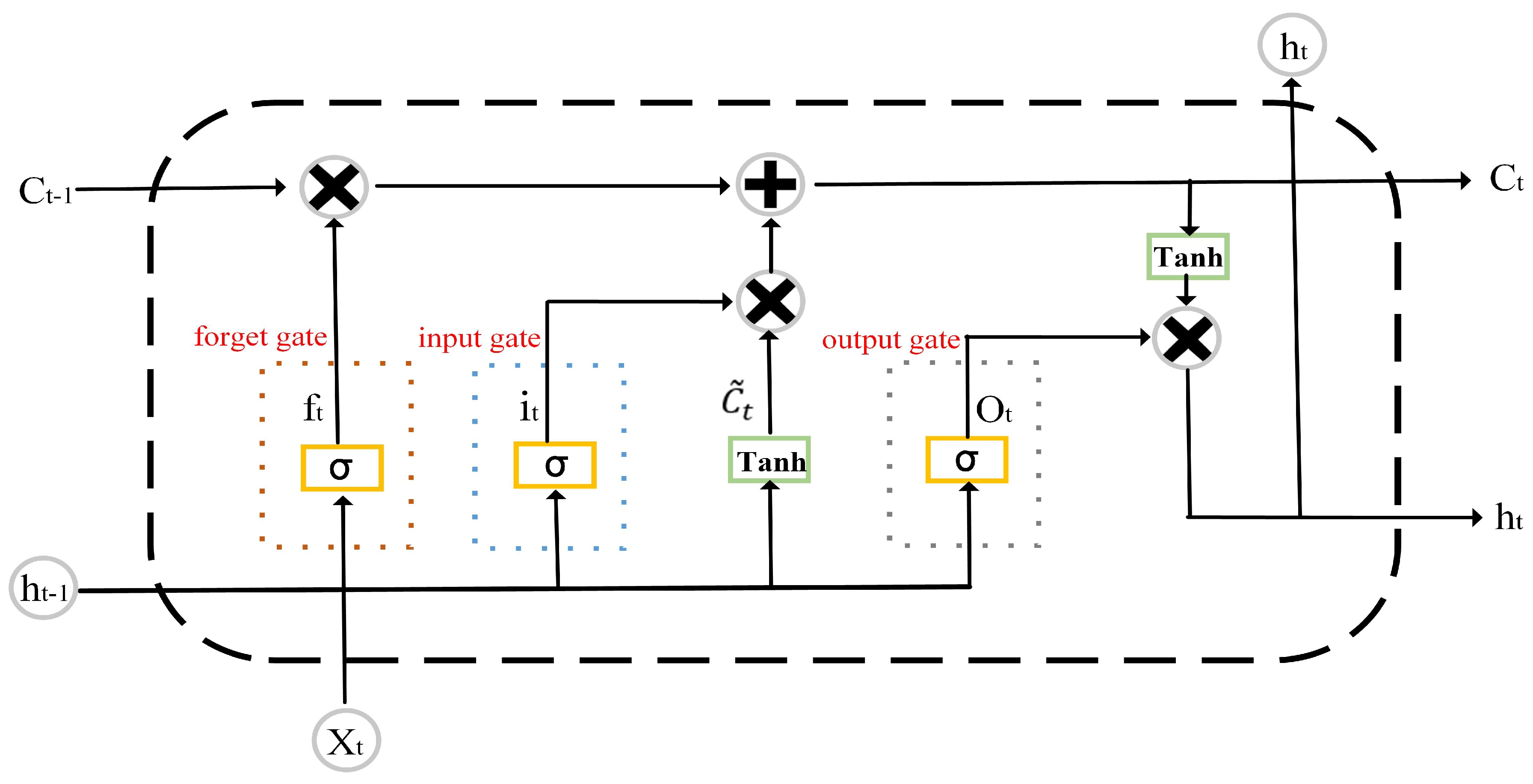
For the nth interference pattern, the low-frequency component in the interference phase is represented as follows:

$$\begin{array}{cc}\hfill \delta {\varphi }_m^{\left(LP\right)}(a,r)& =\frac{4\pi }{\lambda }\left[s^{\left(LP\right)}\left(t_{Mn},a,r\right)-s^{\left(LP\right)}\left(t_{Sn},a,r\right)\right]\hfill \\ \hfill & +\frac{4\pi }{\lambda }\frac{b_{\perp }\Delta e^{\left(LP\right)}(a,r)}{rsin\theta }+\left[{\varphi }^{atmo}\left(t_{Mn},a,r\right)\right.\hfill \\ \hfill & \left.-{\varphi }^{atmo}\left(t_{Sn},a,r\right)\right]+\Delta n_m^{\left(LP\right)}(a,r)\hfill \end{array}$$

(10)

In this equation, $t_{Mn}$, $t_{Sn}$, a, and r represent the time of the main image, the time of the secondary image, the azimuth coordinates, and the distance coordinates, respectively. $s^{\left(LP\right)}$ and $e\left(LP\right)$ represent the LP component of the deformation signal and the terrain error, respectively. $nm\left(LP\right)$ is the noise component, and ${\varphi }^{atmo}(t_{Mn},a,r)-{\varphi }^{atmo}(t_{Sn},a,r)$ represents the atmospheric phase. Additionally, $\lambda$ represents the wavelength of the transmission signal, $b_{\perp }$ is the vertical baseline component, and $\theta$ is the incidence angle. Then, assuming $s^{\left(LP\right)}(t_0,a,r)$ is constant at 0, $\forall (a,r)\in D$, we determine D as the main subject to calculate $s^{\left(LP\right)}(t_n,a,r)$, where $n=0,\dots \dots ,N$ represents the time series of low-pass deformation, and the pixel position $(a,r)$ is calculated relative to the reference time $t_0$.

In the interferogram of the m scene, the residual phase of each pixel is represented as follows: where $V^{\left(HP\right)}$ and ${\beta }^{\left(HP\right)}$ represent the non-linear part of the average rate and residual deformation, $e\left(HP\right)$ is the high-resolution terrain error, and $nm\left(HP\right)$ is the noise term. The calculation formula is shown as follows:

$$\begin{array}{cc}\hfill \delta {\varphi }_m^{\left(HP\right)}(a,r)=& \frac{4\pi }{\lambda }\left[\left(t_{Mn}-t_{Sn}\right)V^{\left(HP\right)}(a,r)+{\beta }^{\left(HP\right)}\left(t_{Mn},a,r\right)-\right.\hfill \\ \hfill & \left.{\beta }^{\left(HP\right)}\left(t_{Sn},a,r\right)\right]+\frac{4\pi }{\lambda }\frac{b_{\perp }\Delta e^{\left(HP\right)}(a,r)}{rsin\theta }+\Delta n_m^{\left(HP\right)}(a,r)\hfill \end{array}$$

(11)

By selecting a few ground points in a region where the interference phase is relatively stable, we can obtain the atmospheric phase and noise components for each scene in the interference dataset. After obtaining the error term, we can use a high-order polynomial interpolation method to interpolate the atmospheric phase in the study area, in order to recover the atmospheric phase and noise components for each scene within the study area. The estimation of $V^{\left(HP\right)}$ and $e\left(PH\right)$ in the residual phase of each pixel in the interferogram of the Nth scene maximizes the time coherence factor ${\gamma }^{\left(HP\right)}(a,r)$, resulting in the following:

$${\gamma }^{\left(HP\right)}(a,r)=\frac{1}{N}\left|\sum _{m=1}^{N}exp\left[j\left(\delta {\phi }_m^{\left(HP\right)}(a,r)\right)-j\delta {\phi }_m(a,r)\right]\right|$$

(12)

In this equation, $\delta {\phi }_m(a,r)$ is a predefined phase residual model, expressed as follows:

$$\delta {\phi }_m(a,r)=\frac{4\pi }{\lambda }\left[\left(t_{Mn}-t_{Sn}\right)V^{\left(HP\right)}(a,r)+\frac{b_{\perp }\Delta e^{\left(HP\right)}(a,r)}{rsin\theta }\right]$$

(13)

In addition, it is estimated that the model error of the high-pass part of the real phase signal is limited to $(-\pi ,\pi )$, and it can be determined that the nonlinear part of the high-pass phase signal and the residual distortion can be simply subtracted by $2\pi$. The rate matrix in the formula is represented as follows:

$$\frac{4\pi }{\lambda }[{\beta }^{\left(HP\right)}(t_{M1},a,r)-{\beta }^{\left(HP\right)}(t_{S1},a,r)]+\Delta n_1^{\left(HP\right)}(a,r)=[\delta {\phi }_1^{\left(HP\right)}(a,r)-\delta {\phi }_1(a,r)]$$

(14)

$$\frac{4\pi }{\lambda }[{\beta }^{\left(HP\right)}(t_{M2},a,r)-{\beta }^{\left(HP\right)}(t_{S2},a,r)]+\Delta n_2^{\left(HP\right)}(a,r)=[\delta {\phi }_2^{\left(HP\right)}(a,r)-\delta {\phi }_2(a,r)]$$

(15)

$$\frac{4\pi }{\lambda }[{\beta }^{\left(HP\right)}(t_{Mn},a,r)-{\beta }^{\left(HP\right)}(t_{Sn},a,r)]+\Delta n_n^{\left(HP\right)}(a,r)=[\delta {\phi }_n^{\left(HP\right)}(a,r)-\delta {\phi }_n(a,r)]$$

(16)

$$v{(a,r)}^T=\left\{\begin{array}{c}{v}_1=\frac{{\beta }^{\left(HP\right)}\left(t_1,a,r\right)-{\beta }^{\left(HP\right)}\left(t_0,a,r\right)}{t_1-t_0}\\ v_{N-1}=\frac{{\beta }^{\left(HP\right)}\left(t_{N-1},a,r\right)-{\beta }^{\left(HP\right)}\left(t_{N-2},a,r\right)}{t_{N-1}-t_{N-2}}\end{array}\right.$$

(17)

Next, the rate vectors in the model can be calculated using the Singular Value Decomposition SVD method.

$$\left\{\begin{array}{c}\sum _{k=S_1+1}^{M_1}\left(t_k-t_{k-1}\right)V_k+\Delta n_1^{\left(HP\right)}(a,r)=\left[\delta {\phi }_1^{\left(HP\right)}(a,r)-\delta {\phi }_1(a,r)\right]\hfill \\ \sum _{k=S_2+1}^{M_2}\left(t_k-t_{k-1}\right)V_k+\Delta n_2^{\left(HP\right)}(a,r)=\left[\delta {\phi }_2^{\left(HP\right)}(a,r)-\delta {\phi }_2(a,r)\right]\hfill \\ \sum _{k=S_n+1}^{M_n}\left(t_k-t_{k-1}\right)V_k+\Delta n_n^{\left(HP\right)}(a,r)=\left[\delta {\phi }_n^{\left(HP\right)}(a,r)-\delta {\phi }_n(a,r)\right]\hfill \end{array}\right.$$

(18)

Using the method of singular value decomposition, we calculate the generalized inverse of the coefficient matrix of the normal equation. This gives me the minimum norm solution for the velocity vector, and allows me to obtain the shape variables for each time period. At this point, the solution is stable, taking into account the influence of noise and minimizing the error in the unfolding process. It also allows for an effective combination of information obtained from different subsets.

3.2. LSTM

LSTM neural networks are derived from traditional RNNs and are widely used for time series modeling [28]. Unlike traditional RNNs, LSTM neural networks have two main modules to help them learn the temporal features of the data. The memory module serves as a cell state, while the gate module consists of an input gate, output gate, and forget gate. The gate module effectively trains the fully connected layers to control the cell state, respond to input from the data, and model the past outputs. For long-term prediction networks, in order to solve the problem of long-term dependencies, it is necessary to remember not only short-term memory but also long-term memory [29,30]. In LSTM neural networks, data information is stored in a separate unit, allowing the LSTM neural network to effectively utilize long-term temporal information [31]. Figure 2 illustrates the basic architecture of LSTM.

According to the network structure of LSTM, the calculation formula for each LSTM unit is as follows: $f_t$ represents the forget threshold, $i_t$ represents the input threshold, ${\tilde{C}}_{t-1}$ represents the previous time step’s cell state, $C_t$ represents the cell state, $O_t$ represents the output threshold, $h_t$ represents the current unit’s output, and $h_{t-1}$ represents the previous time step’s unit’s output. The formula is as follows:

$$f_t=\sigma (W_f·[h_{t-1},x_t]+bf)$$

(19)

$$i_t=\sigma (W_i·[h_{t-1},x_t]+bi)$$

(20)

$${\tilde{C}}_t=tanh\left(W_c·\left[h_{t-1},x_t\right]+b_c\right)$$

(21)

$$C_t=f_t\ast C_{t-1}+i_t\ast {\tilde{C}}_t$$

(22)

$$O_t=\sigma (W_o·[h_{t-1},x_t]+bo)$$

(23)

$$h_t=O_t\ast tanh\left(C_t\right)$$

(24)

The predictive network, constructed using LSTM, is shown in Figure 3. The predictive network consists of two main modules, namely the training module and the prediction module. The training module is primarily used to generate a pre-trained model, while the prediction module is used to run the model and obtain prediction results. The key component of the entire framework is the deep neural network, which includes the input layer, hidden layer, and output layer. The hidden layer is constructed using the LSTM model to learn the temporal features of the time series, while the output layer outputs the prediction results. In this study, we use the settlement sequences obtained from SBAS as the input for the sampling matrix.

The pseudocode for the algorithm is shown in Algorithm 1:

Algorithm 1: Display of overall algorithm structure of motion recognition

3.3. Attention Mechanism

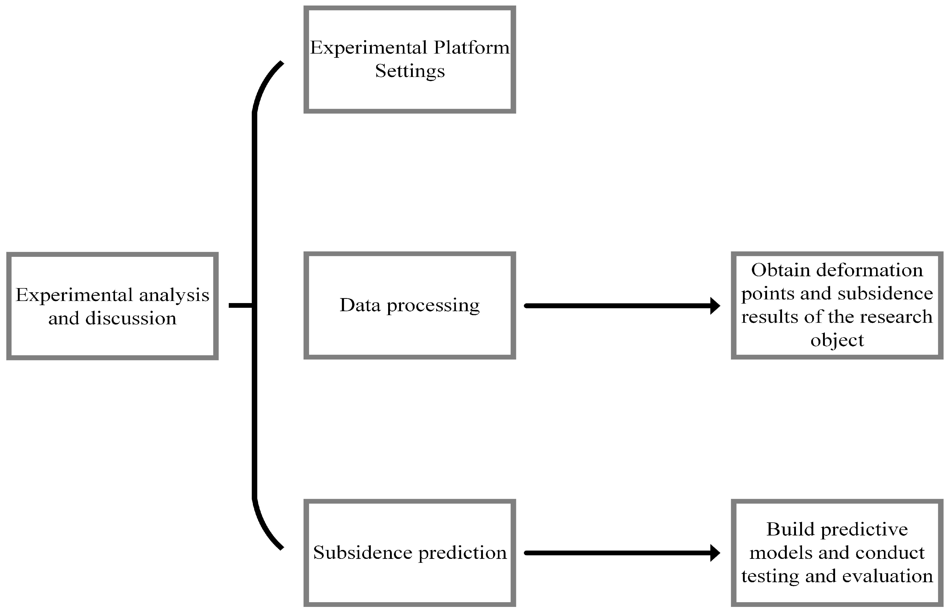
With the development of neural networks, the concept of an attention mechanism has become an important concept in neural networks and has been applied and researched in various fields. The attention mechanism is mainly used to learn the importance of features [32]. It was first proposed in the field of machine translation and was used to assign greater weights to more relevant words in the source language and target language, so that these relevant words would have a greater impact in subsequent calculations. The attention mechanism [33] has achieved high accuracy in many sequence-based tasks, as shown in Figure 4 of the model diagram.

The core of the attention mechanism is to compute attention coefficients between different nodes. First, we use convolutional operations to obtain the feature representations of m nodes, denoted as $h_1\dots h_m$. Then, we calculate the attention coefficients between nodes i and j.

$$a_{ij}=softmax\left(e_{ij}\right)=\frac{exp\left(e_{ij}\right)}{{\sum }_{k\in N_i}{e}_{ik}}$$

(25)

In this equation, W represents the weight matrix. $e_{ij}$ represents the association between node i and node j. $a_{ij}$ normalizes the association $e_{ij}$ using the $softmax$ function. $h_i$ and $h_j$ represent the normalized feature representations of node i and node j, respectively.

The attention mechanism is used to calculate the attention information between nodes as weights, and the decision is made based on the highest weighted parts. However, when the sizes of different data points in the input are inconsistent, it often requires multiple types of convolutional blocks to process inputs of different sizes [34]. When there are too many types of convolutional blocks, training a large number of parameters will lead to high computational costs. The attention mechanism not only takes into account the potential relationships within nodes, but can also handle inputs with variable sizes, greatly reducing the computational costs.

4. Experiment

4.1. Experimental Platform and Settings

The operating system used in the experiment is Windows10 and Intel processor, the chip type is GeForce GTX 1650, the CPU frequency is 2.40 GHz, and the memory is 8 GB. It is used to train on the server with GPU. The algorithm in this paper is based on Python’s deep learning framework, Python version 3.7. The learning rate of the initial training is set to 0.001, and the compilation environment is Pycharm. The experimental flowchart is shown in Figure 5.

We have collected 39 images of Sentinel-1A. The image details are shown in

Table 1. SAR image details.

Parameter	Value
Band	C
Wavelength	5.55 cm
Incidence angle	34.05${}^{\circ }$
Azimuth angle	−166.08${}^{\circ }$
Direction	descending
Sensor mode	IW
Platform	1A
Time span	2020/9–2021/12
Temporal interval	12 days
Number of images	39

, with a time span of 15 months.

4.2. Data Processing

This article focuses on heritage buildings as the research subject. The Sentinel-1A data were processed using the SBAS technique to obtain the deformation points and subsidence time series results of the research subject (as shown in Figure 6, the technical roadmap). The SAR image shows the research area and coverage range (as shown in Figure 7). Based on 39 descending orbit Sentinel-1A images, the SBAS-InSAR technique was used to obtain deformation results in the LOS direction of the InSAR sequence over a period of 15 months. In our research, we particularly focused on the differences in deformation rates at different locations and visualized them through color coding. The results indicate that the deformation rates vary at different locations in the research area, with red indicating the direction away from the satellite (i.e., ground subsidence) and blue indicating the direction towards the satellite (i.e., ground uplift). From the figure, it can be seen that the maximum subsidence rate is −50 mm/year, and the maximum uplift rate is 60 mm/year. It can be observed from the figure that the deformation distribution in the entire research area shows an increase from west to east, indicating a gradual increase in subsidence, which we speculate is due to the terrain. From the figure, it can be seen that the terrain increases from west to east.

In Figure 8, regions A, B, C, and D are clearly identifiable deformation areas. Among them, regions A, C, and D show significant subsidence and have formed subsidence funnels. Region B is classified as an uplift area. Firstly, let us focus on region A. In region A and the northern part of region A, there is significant subsidence with a subsidence rate of up to 60 mm/year. By comparing the historical images of region A, it can be found that, due to rainfall and construction, region A experienced severe settlement, which also led to a significant surface subsidence funnel, further highlighting the severity of the deformation. From the figure, it can be seen that the subsidence distribution in region B is not consistent, and the situation is slightly complex. In region B, uplift is the main deformation, but there is also subsidence. This region not only includes the uplift of the ground, but also is accompanied by some local subsidence. The deformation rate in region B exceeds 20 mm/year, while the surrounding subsidence rate reaches −15 mm/year. There are also stable areas in the surroundings (indicated by the green color, −10 mm/year to 10 mm/year), this inconsistent deformation distribution indicates that the ground motion in region B is very complex, with uplift being one of the main deformation trends, but accompanied by some local settlement phenomena. The deformation of this region may be influenced by multiple factors, and further research is needed to understand its mechanisms; on the other hand, region C is located to the south of region A and exhibits slight ground subsidence, with a subsidence rate of approximately −30 to −20 mm/year. While the degree of subsidence in this area is relatively low, it is still worth noting, as it may have implications for the stability of underground structures and buildings. However, region D shows severe subsidence with a subsidence rate of up to −65 mm/year. From the remote sensing images [35], it can be observed that region D is primarily located around the river channel. Therefore, we speculate that the severe subsidence is due to the instability of underground structures caused by river erosion. This severe land subsidence may pose a potential threat to building communities and infrastructure. In order to further analyze the settlement information of these four areas, we have plotted the cumulative settlement time series for these four regions, as shown in Figure 9.

From the figure, it can be observed that the sampling points in Zone A experienced continuous settlement during the research period, with a cumulative settlement of −60 mm. In Zone B, the sampling points showed a trend of initial subsidence followed by an upward movement, with a significant increase in the latter part of October 2020. In the period from September to October 2020, Zone C exhibited a consistent downward trend, with a relatively uniform decrease in settlement.

However, from October 2020 to the end of 2020, there was a seasonal impact which we infer to be related to winter rainfall and temperature drop. During the period from September 2020 to the end of October 2020, Zone D showed consistent subsidence, but after October 2020, the amplitude of seasonal oscillation increased, with a maximum decrease of 30 mm. Figure 10 illustrates the spatiotemporal evolution of subsidence in the study area during the research period. The distribution of subsidence in the study area is uneven, with the cumulative subsidence increasing from west to east. The time series plot shows that the cumulative subsidence in the study area gradually increases, with a maximum of 100 mm.

4.3. Subsidence Prediction

In this study, a total of 646,894 deformation points were obtained from Sentinel-1A images, and an LSTM model was constructed for subsidence deformation prediction. The dataset was divided into a training set and a test set in an 8:2 ratio. Once the neural network design was completed, the training set was inputted into the network. During the model training process, due to the complexity of the neural network structure, the model was prone to overfitting as the number of iterations increased. Therefore, it was necessary to add a Dropout layer to the LSTM layer of the model to improve its generalization ability and avoid overfitting. The main function of this layer is to randomly drop a certain proportion of neurons in the LSTM layer during each training process [36]. Through experimental testing, it was found that the prediction accuracy of the model did not change with the increase of LSTM layers, and the choice of step size was equally important. In this study, a step size value of three was used, and the next variable was predicted based on the previous three variables. The Units parameter in the LSTM layer represents the number of neurons in that layer, which determines the size of the tensor output from LSTM. The activation function determines the method of activation. A linear activation function was chosen for the LSTM layer, and a Sigmoid activation function was chosen for the dense layer. The combination of these methods can make the model more accurate. The parameter for the Dropout layer was set to 0.2, meaning that 20% of the neurons would be randomly dropped [37,38,39].

In the case of neural network models, there are multiple hyperparameters. These hyperparameters control the structure, efficiency, and functionality of the model, and are crucial for achieving high-precision results. In this experiment, the grid search method was used to adjust the hyperparameters of the model. By setting the range of values for the hyperparameters and evaluating the model based on the growth rate of the hyperparameters, the hyperparameter combination with the best model was selected. In the evaluation of the model, we used the loss rate as the measure, primarily evaluated using Mean Squared Error (MSE). The calculation formula for MSE is as follows:

$$MSE=\sum _{i=1}^n\frac{{({Predicted}_i-{Actual}_i)}^2}{n}$$

(26)

During the training of the model, the fitting degree of the model is judged by measuring the value of the Loss function. When the loss values of the training and testing sets ultimately reach the same level, it is proven that the model has achieved good fitting performance.

The experiment demonstrates that different values of the “Epochs” parameter have an impact on the prediction results. The specific parameter settings are shown in

Table 2. Model parameter setting.

Hyperparameter Name	Value
LSTM_units	48
Batch_size	1
Dropout	0.2
Epochs	260

. For the experiment, we selected a parameter range between 260 and 360. The experimental results indicate that, when the “Epochs” is set to 260, the maximum and minimum loss rates are shown in Figure 11. In the graph, the x-axis represents Epochs and the y-axis represents Loss. It can be observed that, as the Epochs increase, the loss rates for both the training set and the test set become closer. However, the experiment shows that, when the Epochs exceeds 260, the decrease in the loss value becomes slower and the decrease is particularly small. Additionally, the correlation between the predicted data and the actual data gradually decreases. Therefore, we believe that the model has better prediction accuracy when the Epochs are set to 260. The experiment indicates that the model is unable to fit before 260 Epochs, so we selected 260 Epochs.

LSTM was used to fit the time series settlement in the above regions A, B, C, and D, and the fitting results are shown in Figure 12. As can be seen from the figure, the best fit of the model is in region B among the four regions A, B, C, and D. We speculate that, due to the presence of seasonal shocks and the influence of noise, the other regions cannot be well fitted. However, the model captures the local fluctuation characteristics of the time series, especially in regions B and D. From the graph, it can be seen that regions B and D have large fluctuations over time, and the fitting results of the neural network are not significantly different from the original values. If the seasonal trend and noise are eliminated, the fitting results may be even better.

5. Discussion

Amidst the process of modernization, the issue of ground subsidence emerges as a significant concern that demands our utmost attention. It carries the potential for persistent and irreversible impacts, stemming from a web of complex and highly detrimental factors. Thus, the imperative arises to institute a continuous monitoring and predictive framework for heritage site surface subsidence over time. This, in turn, can provide timely references for government interventions in prevention and control. Conventional monitoring approaches are often beset by drawbacks such as time intensiveness and high costs, coupled with limitations in achieving large-scale measurements. In contrast, the utilization of time-series InSAR technology, with its inherent advantages of all-weather suitability, extensive monitoring range, high precision, and its capacity to yield time-series surface subsidence sequences, has progressively evolved into a pivotal technique for surface monitoring. This study combines LSTM and SBAS technologies to assist in decision-making for heritage buildings, providing effective early warning and disaster mitigation, thereby offering valuable insights for ground subsidence hazard prevention in heritage buildings. In our research, we have employed a series of innovative techniques to enhance the accuracy and interpretability of architectural deformation. Firstly, we utilize SBAS-InSAR technology, a powerful remote sensing tool, to process interferometric data from multiple time phases. Compared to traditional methods, SBAS-InSAR is more effective in mitigating nonlinear surface deformations, such as changes in topography and land use. This allows us to capture surface deformation signals more clearly, reducing the impact of noise caused by surface changes in conventional approaches. Next, we introduce Long Short-Term Memory (LSTM) networks, a deep learning technique suitable for time-series data modeling. LSTM networks possess adaptive receptive fields, making them adept at contextual modeling, especially in handling multi-layered, multi-scale, and categorical objects in remote sensing images. In contrast to traditional time-series analysis methods, LSTM networks excel in capturing temporal features and correlations. Finally, we incorporate an attention mechanism, which dynamically selects and weighs features, aiding in the precise capture of critical information within the data. This is particularly crucial in predicting architectural deformation, as deformation characteristics may vary across different regions and time periods. Additionally, the attention mechanism allows for the visualization of focus areas, facilitating our understanding of the key factors driving architectural deformation. In summary, our approach stands out from the existing literature by integrating SBAS-InSAR technology, LSTM networks, and an attention mechanism. This integration enhances the accuracy, interpretability, and adaptability of architectural deformation prediction. In comparison to conventional methods, our approach excels in handling noise and nonlinear deformations within the data, while also accommodating various geographical and meteorological conditions. The application of these innovative techniques positions our approach as a valuable asset in the field of deformation monitoring.

Nevertheless, our method is not devoid of limitations. It necessitates high-quality data and resolutions to ensure the precision of deformation prediction. In some surface deformation scenarios, especially those characterized by low time resolution, like mountain uplift or volcanic eruption, the impact of vertical deformation may, regrettably, be disregarded. Additionally, it is imperative to acknowledge that LSTM exhibits certain limitations, including challenges with long-term dependencies, interpretability issues, and the selection of optimal hyperparameters. These are all aspects that require further refinement and scrutiny in our forthcoming research endeavors as we strive to identify the most suitable model for addressing these challenges.

6. Conclusions

In this research, we harnessed Synthetic Aperture Radar (SAR) images from the Sentinel-1A satellite with reduced orbit data. We employed the Small Baseline Subset (SBAS) Interferometric SAR (InSAR) technique to gather a comprehensive time series of ground subsidence spanning from September 2020 to 2021. Furthermore, we meticulously crafted an LSTM neural network model for predictive analysis. The ensuing outcomes are detailed below:

(1)

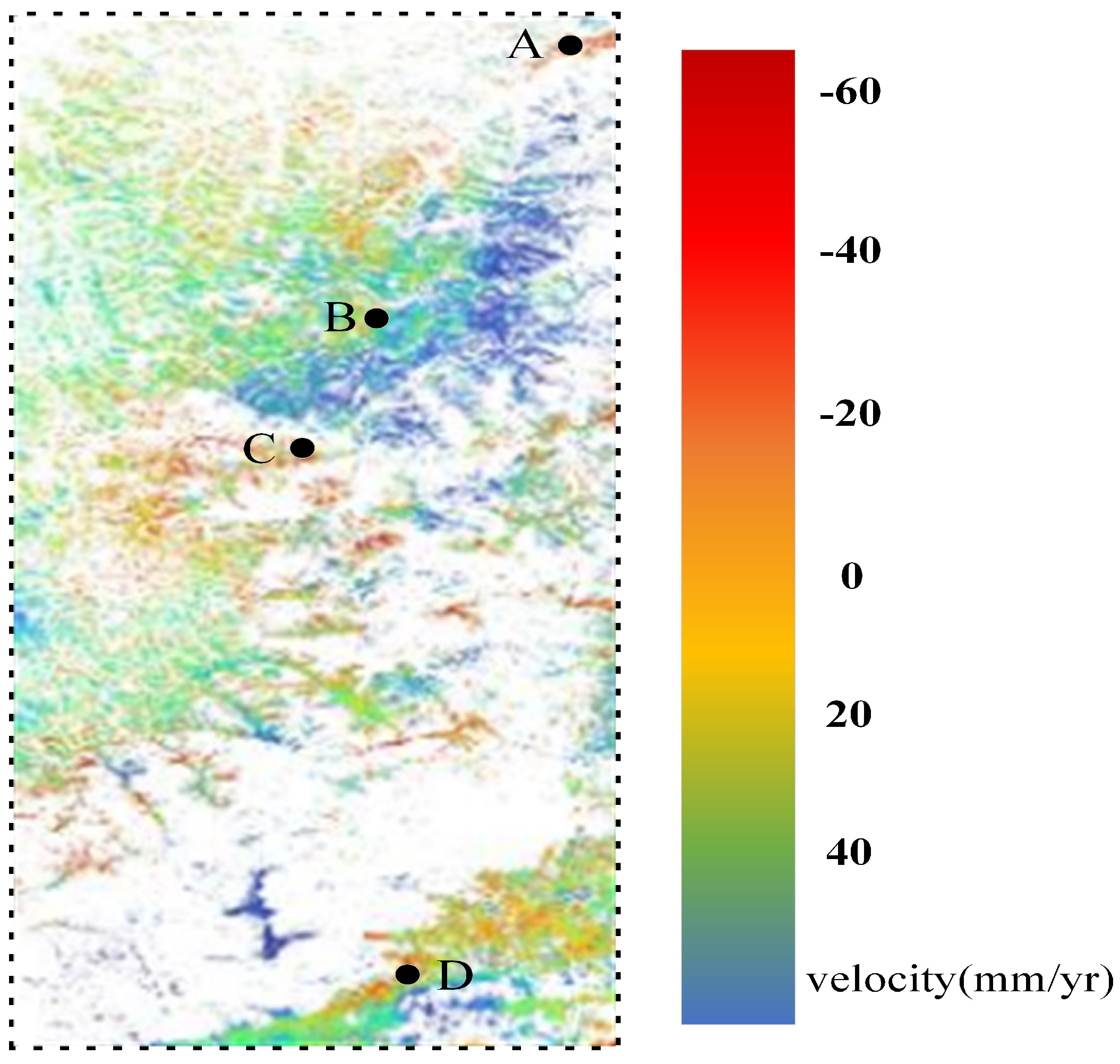
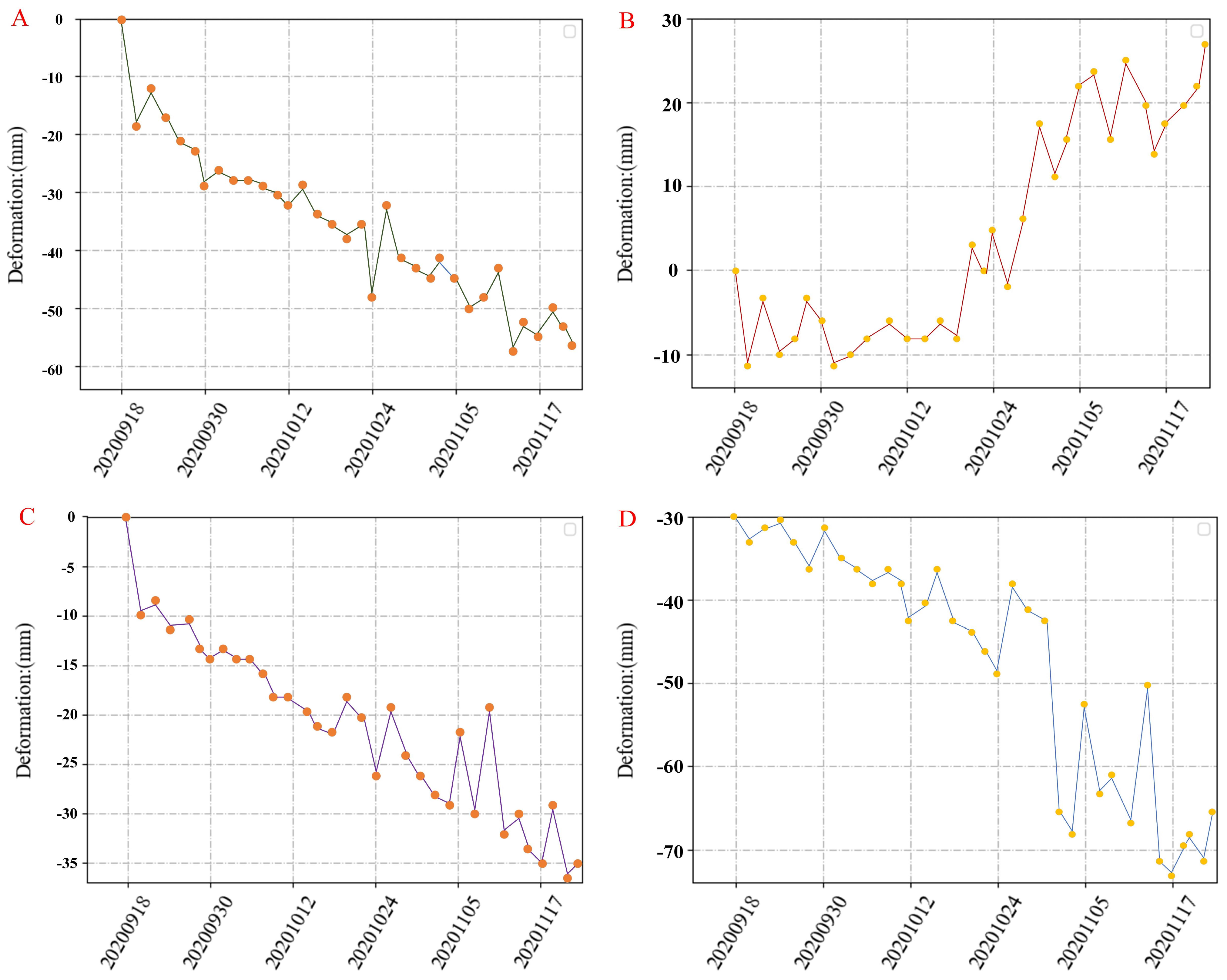
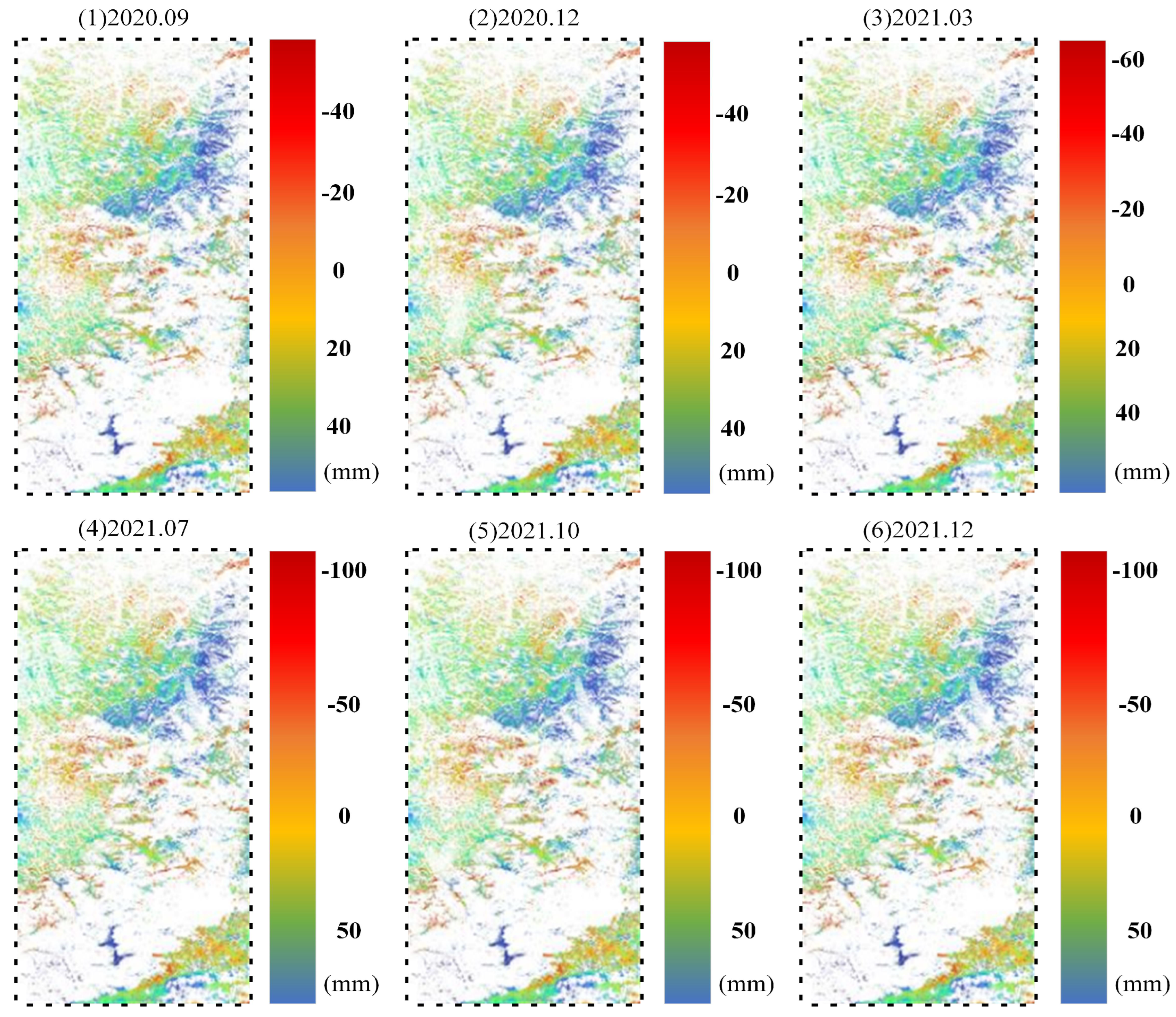
According to the research findings, the subsidence rate in the study area ranged from −65 to 50 mm/year from September 2020 to December 2021, and the land subsidence rate gradually increased. In December 2021, the cumulative subsidence in the Loss direction reached −65 mm. The spatial distribution of ground subsidence in the study area is uneven. The cumulative effects have increased from west to east. These phenomena pose a significant threat to the heritage building in the study area, and ground subsidence is an irreversible geological hazard. Therefore, it is necessary to conduct investigations on the heritage building in the study area and play a proactive role in prevention.

(2)

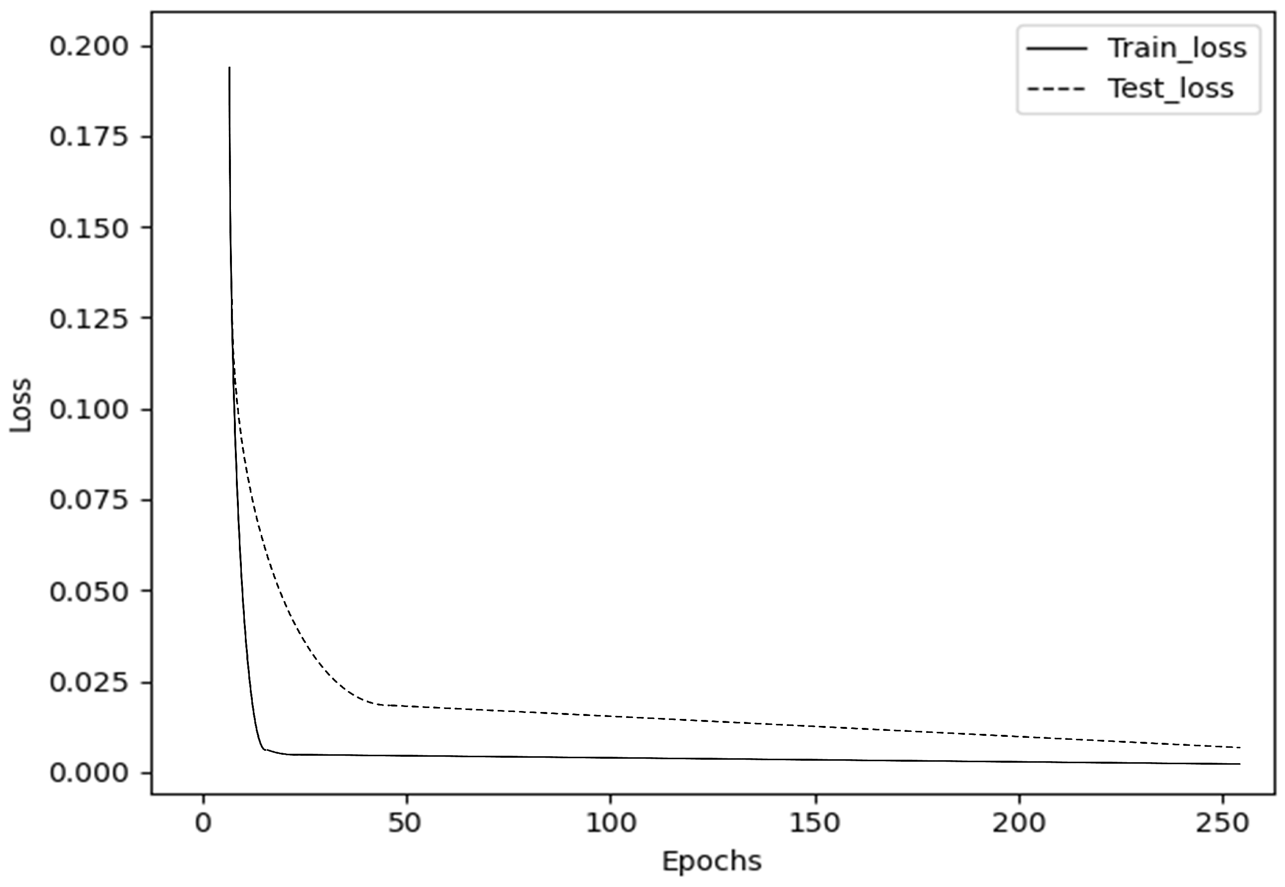
The LSTM neural network prediction model is built based on time series SBAS-InSAR results to predict the dynamic surface subsidence in the mining area using the Richards model. Through model design, training, and parameter selection, the LSTM neural network model achieves relatively high accuracy. However, it cannot learn well due to the noise and seasonal effects in the data. We speculate that this is caused by the uncertainty of seasonal variations and noise.

In future research, we will continuously enhance the model algorithm in this study. We will train multivariate neural networks and eliminate noise and seasonal effects in the source data to achieve a more accurate model. This will help us better understand future ground subsidence predictions.

References

1. Wang, J.; Li, C.; Li, L.; Huang, Z.; Wang, C.; Zhang, H.; Zhang, Z. Insar time-series deformation forecasting surrounding salt lake using deep transformer models. Sci. Total Environ. 2023, 858, 159744. [Google Scholar] [CrossRef]
2. Liu, Y.; Zhang, J. Integrating sbas-insar and at-lstm for time-series analysis and prediction method of ground subsidence in mining areas. Remote Sens. 2023, 15, 3409. [Google Scholar] [CrossRef]
3. Ourang, S. Evaluation of Inter-Organizational Coordination of Housing Services in Rural Alaska through Social Network Analysis. Master’s Thesis, Iowa State University, Ames, IA, USA, 2022. [Google Scholar] [CrossRef]
4. Zhang, M.; Xie, K.; Zhang, Y.-H.; Wen, C.; He, J.-B. Fine segmentation on faces with masks based on a multistep iterative segmentation algorithm. IEEE Access 2022, 10, 75742–75753. [Google Scholar] [CrossRef]
5. Meng, F.; Jagadeesan, L.; Thottan, M. Model-based reinforcement learning for service mesh fault resiliency in a web application-level. arXiv 2021, arXiv:2110.13621. [Google Scholar]
6. Wu, J.; Tao, R.; Zhao, P.; Martin, N.F.; Hovakimyan, N. Optimizing nitrogen management with deep reinforcement learning and crop simulations. In Proceedings of the IEEE/CVF Conference on Computer Vision and Pattern Recognition, New Orleans, LA, USA, 19–20 June 2022; pp. 1712–1720. [Google Scholar]
7. Tang, Z.; Chen, T.; Liu, K.; Du, H.; Podkolzin, S.G. Atomic, molecular and hybrid oxygen structures on silver. Langmuir 2021, 37, 11603–11610. [Google Scholar] [CrossRef]
8. D’Emilia, G.; Gaspari, A.; Marsella, S.; Marzoli, M.; Natale, E. Calibration issues of a total station for the assessment of buildings in emergency conditions. In Proceedings of the 2022 IEEE International Workshop on Metrology for Living Environment (MetroLivEn), Cosenza, Italy, 25–27 May 2022; pp. 81–85. [Google Scholar]
9. Vadivel, S.K.P.; Kim, D.-J. Urban subsidence monitoring in pohang city using time-series insar technique. In Proceedings of the 2022 13th International Conference on Information and Communication Technology Convergence (ICTC), Jeju Island, Republic of Korea, 19–21 October 2022; pp. 913–916. [Google Scholar]
10. Dong, L.K.; Tang, F.Q. Experimental research on radar remote sensing monitoring of coal mining subsidence in loess mining area. In Proceedings of the 2018 Fifth International Workshop on Earth Observation and Remote Sensing Applications (EORSA), Xi’an, China, 18–20 June 2018; pp. 1–5. [Google Scholar]
11. Li, Z.; Wu, Q.; Cheng, B.; Cao, L.; Yang, H. Remote sensing image scene classification based on object relationship reasoning cnn. IEEE Geosci. Remote. Sens. Lett. 2020, 19, 1–5. [Google Scholar] [CrossRef]
12. Zhang, Y.-H.; Wen, C.; Zhang, M.; Xie, K.; He, J.-B. Fast 3d visualization of massive geological data based on clustering index fusion. IEEE Access 2022, 10, 28821–28831. [Google Scholar] [CrossRef]
13. Zhang, X.; Li, Z.; Liu, Z. Reduction of atmospheric effects on insar observations through incorporation of gacos and pca into small baseline subset insar. IEEE Trans. Geosci. Remote Sens. 2023, 61, 5209115. [Google Scholar] [CrossRef]
14. Mao, W.; Wang, X.; Liu, G.; Pirasteh, S.; Zhang, R.; Lin, H.; Xie, Y.; Xiang, W.; Ma, Z.; Ma, P. Time series insar ionospheric delay estimation, correction, and ground deformation monitoring with reformulating range split-spectrum interferometry. IEEE Trans. Geosci. Remote Sens. 2023, 61, 5213118. [Google Scholar] [CrossRef]
15. Bassolia, E.; Grassia, F.; Varzaneha, G.E.; Ponsi, F.; Mancini, F.; Vincenzi, L. A simplified procedure to assess uncertainties in the estimation of the rigid motion of isolated buildings based on insar monitoring. Procedia Struct. Integr. 2023, 44, 1554–1561. [Google Scholar] [CrossRef]
16. Li, L.; Wen, B.; Yao, X.; Zhou, Z.; Zhu, Y. Insar-based method for monitoring the long-time evolutions and spatial-temporal distributions of unstable slopes with the impact of water-level fluctuation: A case study in the xiluodu reservoir. Remote Sens. Environ. 2023, 295, 113686. [Google Scholar] [CrossRef]
17. Wang, H.; Jia, C.; Ding, P.; Feng, K.; Yang, X.; Zhu, X. Analysis and prediction of regional land subsidence with insar technology and machine learning algorithm. KSCE J. Civ. Eng. 2023, 27, 782–793. [Google Scholar] [CrossRef]
18. Zan, F.D.; Saporta, P.; Gomba, G. Spatiotemporal analysis of c-band interferometric phase anomalies over sicily. In Proceedings of the EUSAR 2022; 14th European Conference on Synthetic Aperture Radar, Leipzig, Germany, 25–27 July 2022; pp. 1–4. [Google Scholar]
19. Fan, H.; Cheng, D.; Deng, K.; Chen, B.; Zhu, C. Subsidence monitoring using d-insar and probability integral prediction modelling in deep mining areas. Surv. Rev. 2015, 47, 438–445. [Google Scholar] [CrossRef]
20. Xiong, S.; Zeng, Q.; Jiao, J.; Gao, S.; Zhang, X. Improvement of ps-insar atmospheric phase estimation by using wrf model. In Proceedings of the 2014 IEEE Geoscience and Remote Sensing Symposium, Quebec City, QC, Canada, 13–18 July 2014; pp. 2225–2228. [Google Scholar]
21. Serva, S.; Fiorentino, C.; Covello, F. The cosmo-skymed seconda generazione key improvements to respond to the user community needs. In Proceedings of the 2015 IEEE International Geoscience and Remote Sensing Symposium (IGARSS), Milan, Italy, 26–31 July 2015; pp. 219–222. [Google Scholar]
22. Geudtner, D.; Miranda, N.; Navas-Traver, I.; Vega, F.C.; Prats, P.; Yague-Martinez, N.; Breit, H.; Zan, F.D.; Larsen, Y.; Recchia, A.; et al. Sentinel-1a/b sar and insar performance. In Proceedings of the EUSAR 2018; 12th European Conference on Synthetic Aperture Radar, Aachen, Germany, 4–7 June 2018; pp. 1–5. [Google Scholar]
23. He, S.; Wang, J.; Yang, F.; Chang, T.-L.; Tang, Z.; Liu, K.; Liu, S.; Tian, F.; Liang, J.-F.; Du, H.; et al. Bacterial detection and differentiation of staphylococcus aureus and escherichia coli utilizing long-period fiber gratings functionalized with nanoporous coated structures. Coatings 2023, 13, 778. [Google Scholar] [CrossRef]
24. Liu, H.; Yuan, M.; Li, M.; Li, B.; Zhang, H.; Wang, J. An efficient and fully refined deformation extraction method for deriving mining-induced subsidence by the joint of probability integral method and sbas-insar. IEEE Trans. Geosci. Remote Sens. 2023, 61, 5208717. [Google Scholar] [CrossRef]
25. Meng, F.; Zhang, L.; Wang, Y. Fedemb: An efficient vertical and hybrid federated learning algorithm using partial network embedding. 2023; anonymous preprint under review. [Google Scholar]
26. Berardino, P.; Fornaro, G.; Lanari, R.; Sansosti, E. A new algorithm for surface deformation monitoring based on small baseline differential sar interferograms. IEEE Trans. Geosci. Remote Sens. 2002, 40, 2375–2383. [Google Scholar] [CrossRef]
27. Graves, A.; Graves, A. Long short-term memory. In Supervised Sequence Labelling with Recurrent Neural Networks; Springer: Berlin, Germany, 2012; pp. 37–45. [Google Scholar]
28. Kawakami, K. Supervised Sequence Labelling with Recurrent Neural Networks. Ph.D. Dissertation, Technical University of Munich, Munich, Germany, 2008. [Google Scholar]
29. He, J.-Y.; Wu, X.; Cheng, Z.-Q.; Yuan, Z.; Jiang, Y.-G. Db-lstm: Densely-connected bi-directional lstm for human action recognition. Neurocomputing 2021, 444, 319–331. [Google Scholar] [CrossRef]
30. Fan, C.; Li, Y.; Yi, L.; Xiao, L.; Qu, X.; Ai, Z. Multi-objective lstm ensemble model for household short-term load forecasting. Memetic Comput. 2022, 14, 115–132. [Google Scholar] [CrossRef]
31. Chen, K.; Zhou, Y.; Dai, F. A lstm-based method for stock returns prediction: A case study of china stock market. In Proceedings of the 2015 IEEE International Conference on Big Data (Big Data), Santa Clara, CA, USA, 29 October–1 November 2015; pp. 2823–2824. [Google Scholar]
32. Liu, K.; Chen, T.; He, S.; Robbins, J.P.; Podkolzin, S.G.; Tian, F. Observation and identification of an atomic oxygen structure on catalytic gold nanoparticles. Angew. Chem. 2017, 129, 13132–13137. [Google Scholar] [CrossRef]
33. Du, Y.; Du, L.; Li, L. An sar target detector based on gradient harmonized mechanism and attention mechanism. IEEE Geosci. Remote Sens. Lett. 2021, 19, 1–5. [Google Scholar] [CrossRef]
34. Moeinifard, P.; Rajabi, M.S.; Bitaraf, M. Lost vibration test data recovery using convolutional neural network: A case study. arXiv 2022, arXiv:2204.05440. [Google Scholar]
35. Wu, J.; Hovakimyan, N.; Hobbs, J. Genco: An auxiliary generator from contrastive learning for enhanced few-shot learning in remote sensing. arXiv 2023, arXiv:2307.14612. [Google Scholar]
36. Fu, R.; Zhang, Z.; Li, L. Using lstm and gru neural network methods for traffic flow prediction. In Proceedings of the 2016 31st Youth Academic Annual Conference of Chinese Association of Automation (YAC), Wuhan, China, 11–13 November 2016; pp. 324–328. [Google Scholar]
37. Kong, W.; Dong, Z.Y.; Jia, Y.; Hill, D.J.; Xu, Y.; Zhang, Y. Short-term residential load forecasting based on lstm recurrent neural network. IEEE Trans. Smart Grid 2017, 10, 841–851. [Google Scholar] [CrossRef]
38. Qu, X.; Yang, J.; Chang, M. A deep learning model for concrete dam deformation prediction based on rs-lstm. J. Sens. 2019, 2019, 4581672. [Google Scholar] [CrossRef]
39. Bao, X.; Zhang, R.; Shama, A.; Li, S.; Xie, L.; Lv, J.; Fu, Y.; Wu, R.; Liu, G. Ground deformation pattern analysis and evolution prediction of shanghai pudong international airport based on psi long time series observations. Remote Sens. 2022, 14, 610. [Google Scholar] [CrossRef]
Figure 1. Overall flow chart of algorithm. Module (A) extracts ground deformation information from SAR image data using SBAS-InSAR technology, resulting in high-precision deformation data. Module (B) employs an LSTM neural network, combined with an attention mechanism, to predict deformations, continuously optimizing the model to enhance prediction capabilities. Module (C) utilizes a trained LSTM model to predict deformations in new data, assesses model accuracy, and provides deformation forecasts for surface monitoring and disaster prevention. This comprehensive algorithm integrates SBAS-InSAR technology and deep learning methods, offering an effective tool for high-precision deformation prediction.
Electronics 12 04724 g001
Figure 2. Structural framework of LSTM.
Electronics 12 04724 g002
Figure 3. Prediction framework of LSTM.
Electronics 12 04724 g003
Figure 4. Attention mechanism model diagram.
Electronics 12 04724 g004
Figure 5. Experimental flow chart.
Electronics 12 04724 g005
Figure 6. Technical route of LSTM prediction.
Electronics 12 04724 g006
Figure 7. Study area map. (a) Represents the province under study, with dashed boxes indicating the coverage range of SAR images. (b) Indicates that the terrain being studied gradually increases from west to east.
Electronics 12 04724 g007
Figure 8. Display of deformation rate in the study area. In Area A, the sampled points exhibited continuous subsidence throughout the study period, resulting in a significant surface subsidence funnel. In Area B, the sampled points displayed a trend of initial subsidence followed by uplift. This inconsistent deformation distribution suggests that ground motion in Area B is highly complex, with uplift being one of the major deformation trends. Area C, located to the south of Area A, experienced slight ground subsidence. Area D, primarily situated around the river channel, exhibited severe subsidence due to unstable underground structures.
Electronics 12 04724 g008
Figure 9. Cumulative time series deformation of the study area. In (A), the sampled points experienced continuous subsidence during the study period, with a cumulative subsidence of approximately −60 mm. In (B), the sampled points showed an initial subsidence followed by a significant uplift from the end of October 2020 until the end of the study period. (C) exhibited consistent and relatively uniform subsidence throughout the study. From October 2020 to the end of the year, a seasonal impact was observed. In (D), continuous subsidence was observed.
Electronics 12 04724 g009
Figure 10. Cumulative settlement in the study area.
Electronics 12 04724 g010
Figure 11. The loss function of the training set and test set is compared. When the value of epochs is 260, the loss function value of both approaches 0.
Electronics 12 04724 g011
Figure 12. Settlement fitting results based on LSTM prediction.
Electronics 12 04724 g012