

Design and Implementation of Omnidirectional Mobile Robot for Materials Handling among Multiple Workstations in Manufacturing Factories


Abstract
:1. Introduction
2. Functional Description of the Designed Feeding Robot
3. Mechanical System Design
3.1. Overall Design
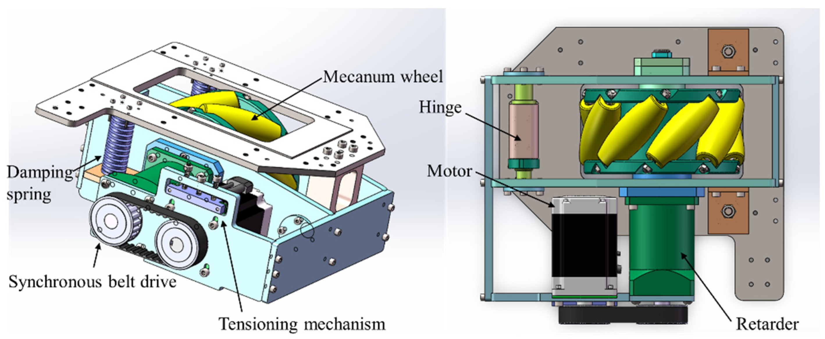
3.1.1. Moving Part
3.1.2. Control Part
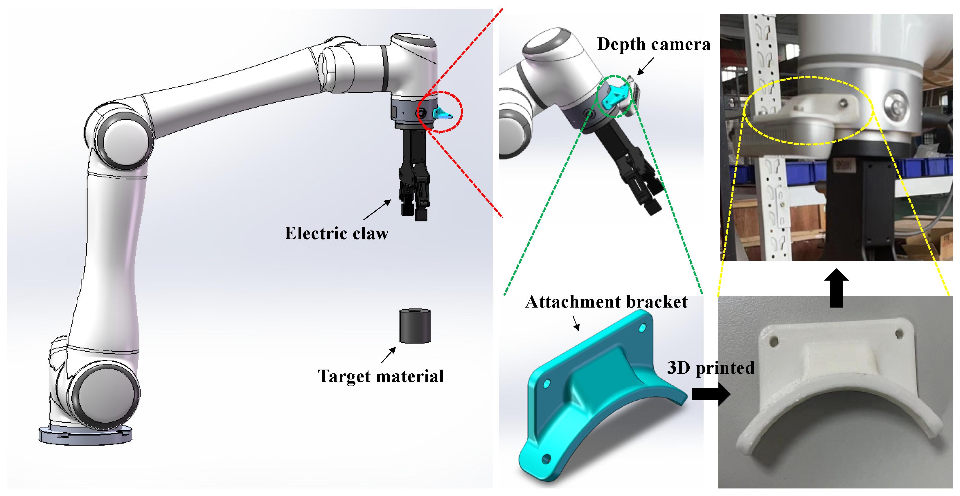
3.1.3. Grabbing Part
3.2. Design of Damping Suspension
4. Kinematic Modeling and Navigation Algorithms
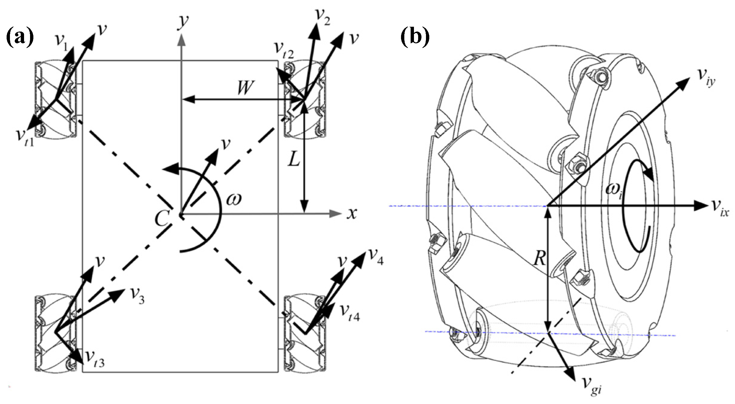
4.1. Kinematic Modeling of Mobile Platform
- (1)
- The ground is level and smooth, and the movement of the mobile platform is carried out on the level and smooth ground.
- (2)
- The mecanum wheels do not slip relative to the ground, and all four wheels have good contact with the ground.
- (3)
- The contact between the mecanum wheel and ground is rigid, and there is no deformation on both contact surfaces.
- (4)
- The wheels are free from wear during operation, and the radii of the four wheels should be exactly the same.
4.2. Navigation Algorithm
5. Control System Design
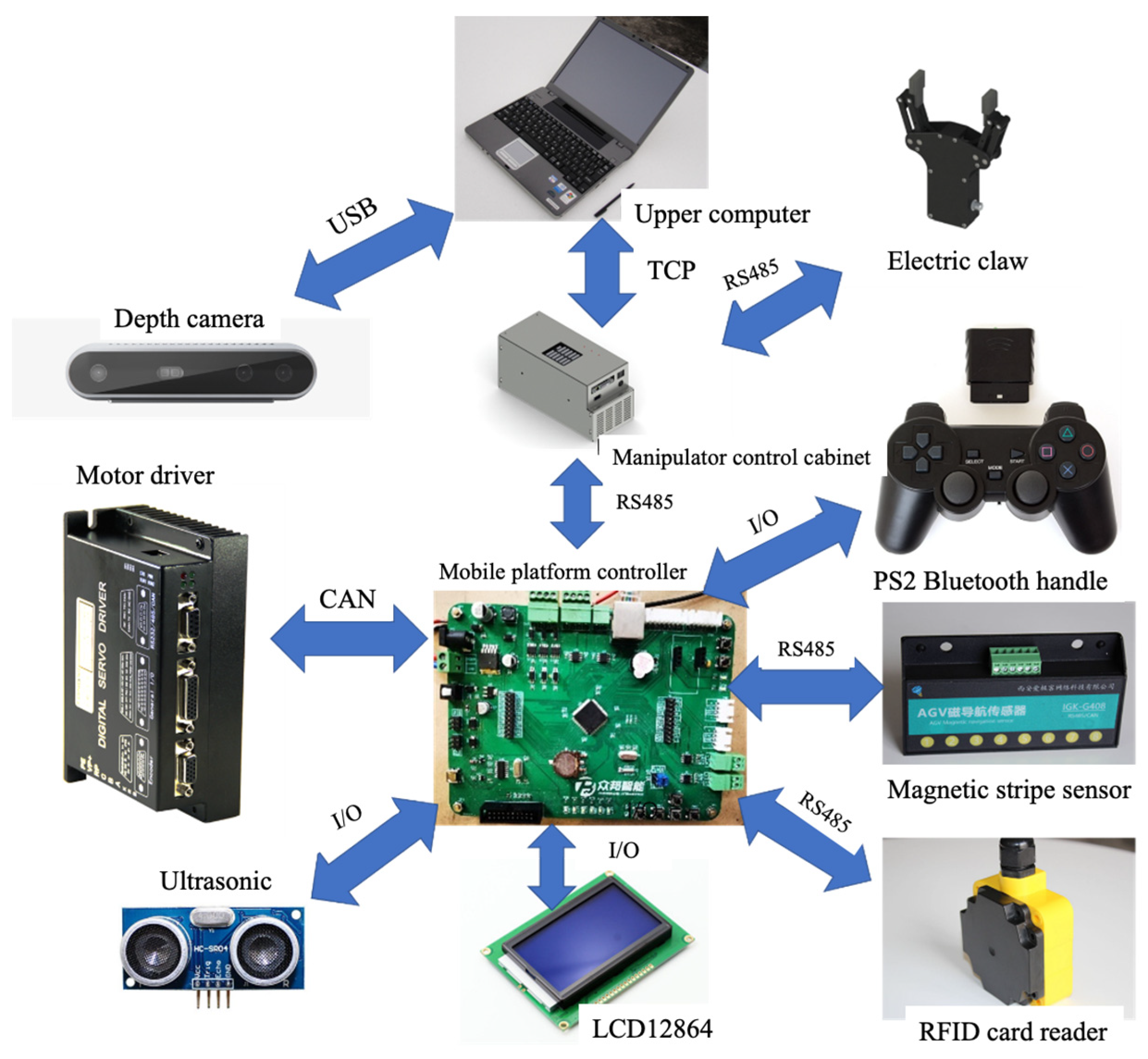
5.1. Overall Structure of Control System
5.2. Hardware Design
- (1)
- Power supply module. Three different voltage modules are needed by the controller, which supply power to the LED indicator light, the minimum system of STM32 single-chip computer, and various functional modules, respectively.
- (2)
- Buzzer module. It is mainly used to generate alarm signals to alert passers-by during the operation of the robot.
- (3)
- USB serial port module. It is mainly used for communication between the controller and the computer. During debugging, the debugging information is printed on the computer display screen. At the same time, a serial port download program can be carried out.
- (4)
- RS485 communication module. It is used for the controller to communicate with the magnetic strip sensor, RFID card reader, and other sensors to obtain sensor data information.
- (5)
- CAN communication module. Used to communicate with the four motor drivers, control the speed of the motor, and obtain information about the current speed of the motor.
- (6)
- Debugging the circuit. Used for program simulation and debugging.
- (7)
- I/O interface. Used to communicate with the LCD, ultrasound module, and PS2 Bluetooth handle receiver.
- (8)
- LED lamp drive module. Used to control the 24V LED indicator light on and off.
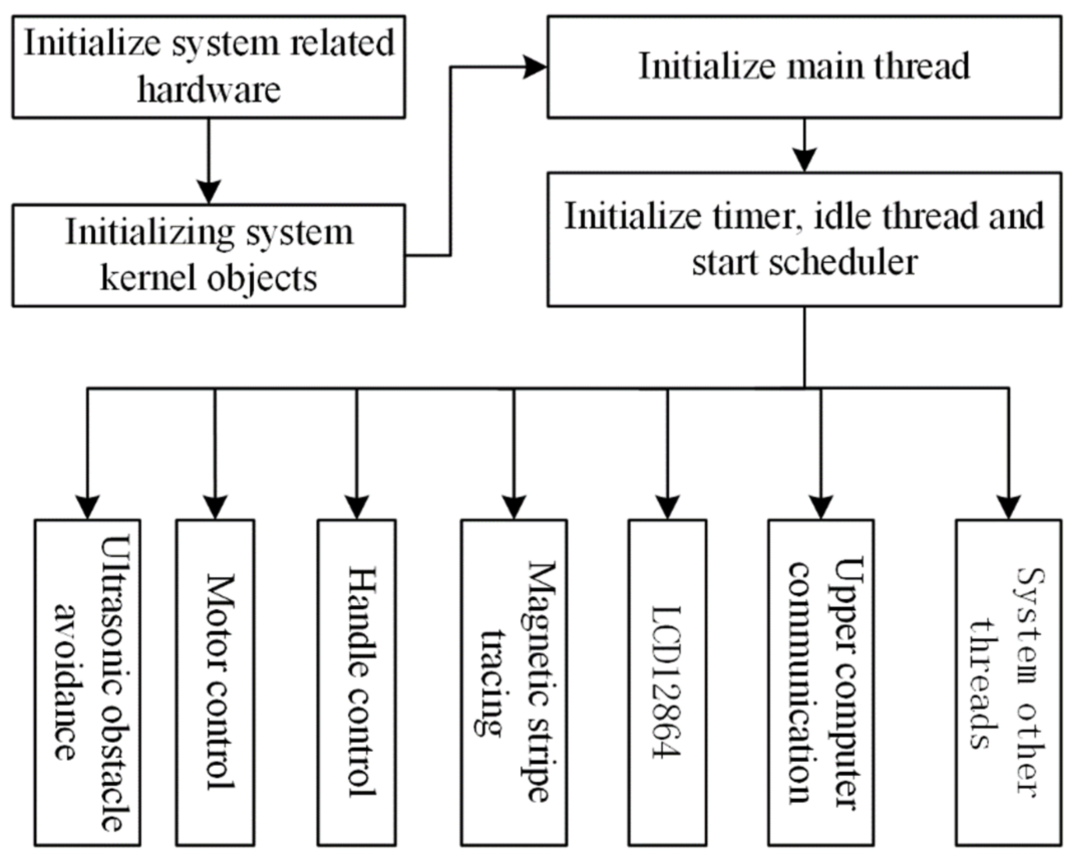
5.3. Software Design
5.3.1. CANopen Motor Control
5.3.2. Function Modules
5.3.3. Design of Slave Station for Communication with Control Cabinet of Robot Arm
6. Grabbing Realization of Mobile Robot
- (1)
- Set up the hardware and software environment of the grab system, including the installation mode of the mechanical arm, camera, and electric claw; the design of the communication program of the electric claw; and the mechanical arm.
- (2)
- Calibrate the robot arm and camera’s hand and eye, and obtain the transformation matrix from the camera coordinate system to the tool coordinate system at the end of the robot arm. After coordinate transformation, the position coordinate of the object under the basic coordinate system of the machine arm is finally obtained.
- (3)
- Find a suitable image recognition algorithm to obtain the object’s pixel coordinates. Through the Realsense D415 depth camera, the object’s three-dimensional spatial coordinates in the camera coordinate system can be read according to the pixel coordinates.
- (4)
- In the grabbing position, according to the cylindrical feature of the grabbing part, the vertical down grabbing position is adopted, as shown in Figure 13.
- (5)
- During the process of grasping, the grasping path of the mechanical arm is planned.
6.1. Hand-Eye Calibration
6.2. Image Recognition
7. Prototype Construction and Experiment
7.1. Prototype Construction and Software Implementation
7.2. Accuracy Test
7.2.1. Hand-Eye Calibration Accuracy Test
7.2.2. Positioning Accuracy Test
7.2.3. Obstacle Avoidance Distance Test
7.2.4. Automatic Correction against Moving Interference Test
7.3. Feeding Experiment
8. Conclusions
- (1)
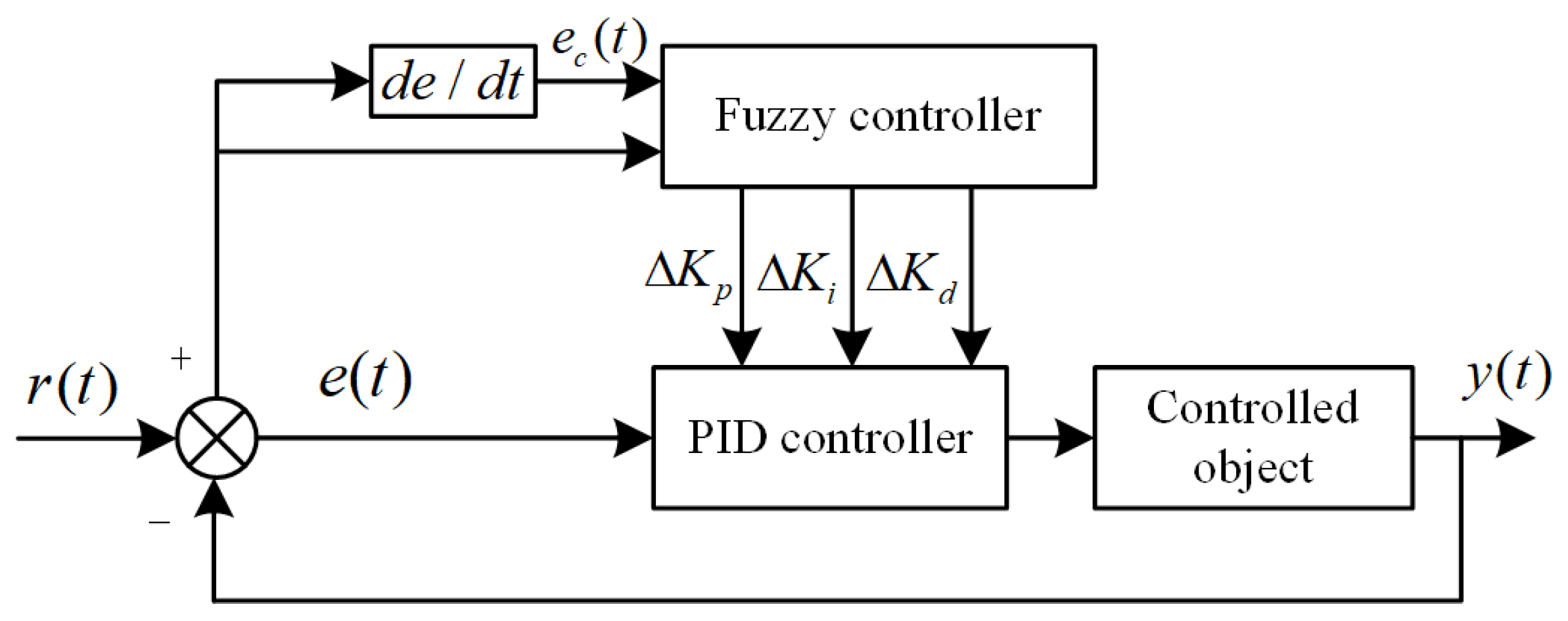
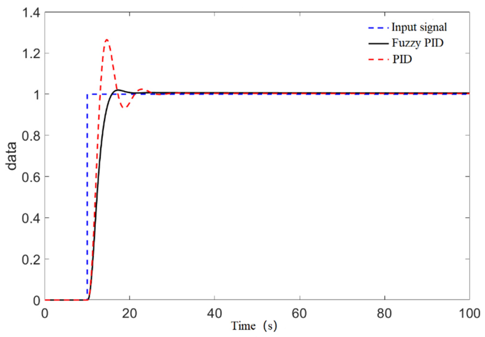
- Through structural optimization and vibration damping solutions, the kinematic model of the robot was established. By using a fuzzy PID control algorithm, the issue of trajectory deviation during tracking due to disturbances was effectively mitigated. The robot exhibits an average repeatability positioning error of approximately 12.95 mm. In the range of (−15, 15), the trajectory deviation adjustment time is under 4.9 s, and the adjustment distance is within 1.16 m, meeting the stipulated design requirements.
- (2)
- The mechanical structure for robot grasping was designed, and hand-eye calibration was performed on the robotic arm and camera when establishing the hand-eye matrix. Through four steps of median filtering, HSV threshold segmentation, morphological processing, and gradient Hough circle transform edge detection, the material part image was recognized and successfully positioned. Localization accuracy falls within a 5.5 mm margin, satisfying the requisite grasping precision requirement.
- (3)
- Ultrasonic obstacle avoidance functionality was implemented using the HC-SR04 ultrasonic module. The mobile robot attains an average obstacle avoidance distance of 345.95 mm, meeting safety protection requirements.
- (4)
- The complete physical assembly of the robot was realized alongside the development of upper computer software for robot feeding. The feeding experiment was effectively implemented.
Author Contributions
Funding
Data Availability Statement
Conflicts of Interest
References
- Srinivasa, S.S.; Berenson, D.; Cakmak, M.; Collet, A.; Dogar, M.R.; Dragan, A.D.; Knepper, R.A.; Niemueller, T.; Strabala, K.; Vande Weghe, M. Herb 2.0: Lessons learned from developing a mobile manipulator for the home. Proc. IEEE 2012, 100, 2410–2428. [Google Scholar] [CrossRef]
- Guo, S.; Jin, Y.; Bao, S.; Xi, F.F. Accuracy analysis of omnidirectional mobile manipulator with mecanum wheels. Adv. Manuf. 2016, 4, 363–370. [Google Scholar] [CrossRef]
- Niu, Z.; Lu, Q.; Cui, Y.; Sun, Z. Fuzzy control strategy for course correction of omnidirectional mobile robot. Int. J. Control Autom. Syst. 2019, 17, 2354–2364. [Google Scholar]
- Wang, Z.; Guo, X.; Wang, H.; Li, H.; Ding, J. AGV positioning and magnetic navigation based on RFID. Equip. Manuf. Technol. 2021, 7, 106–110. [Google Scholar]
- Zhao, J.; Li, D.; Wang, C. PID fuzzy controller and measurement research of magnetic navigation AGV based on Mitsubishi PLC. Meas. Control Technol. 2019, 38, 146–150. [Google Scholar]
- Hua, T. The Design and Realization of Magnetic Guided Omnidirectional AGV Based on Fuzzy PID Compound Control. Ph.D. Thesis, Huazhong University of Science & Technology, Wuhan, China, 2017. [Google Scholar]
- Lu, Y.; Huang, G. Positioning and Navigation of Meal Delivery Robot Using Magnetic Sensors and RFID. In Proceedings of the 2014 International Symposium on Computer, Consumer and Control, Taichung, Taiwan, 10–12 June 2014; pp. 808–811. [Google Scholar]
- Miao, J.; Niu, L. Design of path tracking control system for magnetic navigation AGV. Modul. Mach. Tool Autom. Manuf. Tech. 2021, 9, 107–116. [Google Scholar]
- Yang, F.; Li, P.; Liu, G.; Wang, W. A new identification and location method and experiment research on a kind of orange harvesting robots. J. Xi’an Univ. Technol. 2018, 34, 460–467. [Google Scholar]
- Budiharto, W. Robust Vision-Based Detection and Grasping Object for Manipulator Using SIFT Keypoint Detector. In Proceedings of the International Conference on Advanced Mechatronic Systems IEEE, Kumamoto, Japan, 10–12 August 2014; pp. 448–452. [Google Scholar]
- Li, Z.; Li, S.; Bai, Q.; Song, Q.; Zhang, X. Research on robot target grabbing based on vision. Modul. Mach. Tool Autom. Manuf. Tech. 2020, 9, 108–111. [Google Scholar]
- Lyu, D.; Xia, H.; Wang, C. Research on the effect of image size on real-time performance of robot vision positioning. EURASIP J. Image Video Process. 2018, 2018, 112. [Google Scholar] [CrossRef]
- Jiao, X.; Guo, W. Design and analysis of wireless remote control omnidirectional mobile transfer platform based on mecanum wheel. Hoisting Conveying Mach. 2021, 1, 49–54. [Google Scholar]
- Mai, T.A.; Dang, T.S.; Duong, D.T.; Le, V.C.; Banerjee, S. A combined backstepping and adaptive fuzzy PID approach for trajectory tracking of autonomous mobile robots. J. Braz. Soc. Mech. Sci. Eng. 2021, 43, 156. [Google Scholar] [CrossRef]
- Marturi, N.; Kopicki, M.; Rastegarpanah, A.; Rajasekaran, V.; Adjigble, M.; Stolkin, R.; Leonardis, A.; Bekiroglu, Y. Dynamic grasp and trajectory planning for moving objects. Auton. Robot. 2019, 43, 1241–1256. [Google Scholar] [CrossRef]
- Song, H.; Wang, G.; Zong, C.; Zhong, P. Analysis and research of location and grabbing scheme based on binocular vision recognition. Mech. Electr. Eng. Technol. 2020, 49, 34–35. [Google Scholar]
- Trivedi, J.; Devi, M.S.; Dhara, D. OpenCV and Matlab Based Car Parking System Module for Smart City Using Circle Hough Transform. In Proceedings of the 2017 International Conference on Energy, Communication, Data Analytics and Soft Computing (ICECDS), Chennai, India, 1–2 August 2017; pp. 2461–2464. [Google Scholar]
- Tang, Q.; Tang, C.; Zhang, H. An improved accurate circle detection method based on hough transform. Aeronaut. Comput. Tech. 2017, 47, 58–61. [Google Scholar]
- Li, Q.; Wu, M. An Improved Hough Transform for Circle Detection Using Circular Inscribed Direct Triangle. In Proceedings of the 2020 13th International Congress on Image and Signal Processing, BioMedical Engineering and Informatics (CISP-BMEI) 2020, Chengdu, China, 17–19 October 2020; pp. 203–207. [Google Scholar]
- Djekoune, A.O.; Messaoudi, K.; Amara, K. Incremental circle hough transform: An improved method for circle detection. J. Light-Electronoptic 2017, 133, 17–31. [Google Scholar] [CrossRef]


| Parameters | Design Requirements |
|---|---|
| Mobile platform size (mm) | 800 × 1300 |
| Mobile platform speed (m/s) | 0.8 |
| Mechanical arm end load (kg) | ≤6 |
| Mobile platform total load (kg) | 500 |
| Working radius of the robot arm (mm) | ≥500 |
| Turning radius (mm) | 0 |
| Obstacle avoidance distance (mm) | >300 |
| Positional accuracy (mm) | 20 |
| E | EC | ||||||
|---|---|---|---|---|---|---|---|
| NB | NS | NM | ZO | PS | PM | PB | |
| NB | PB | PB | PM | PM | PS | PS | ZO |
| NM | PB | PB | PM | PM | PS | ZO | ZO |
| NS | PM | PM | PM | PS | ZO | NS | NM |
| ZO | PM | PS | PS | ZO | NS | NM | NM |
| PS | PS | PS | ZO | NS | NS | NM | NM |
| PM | ZO | ZO | NS | NM | NM | NM | NB |
| PB | ZO | NS | NS | NM | NM | NB | NB |
| E | EC | ||||||
|---|---|---|---|---|---|---|---|
| NB | NS | NM | ZO | PS | PM | PB | |
| NB | NB | NB | NB | NM | NM | ZO | ZO |
| NM | NB | NB | NM | NM | NS | ZO | ZO |
| NS | NM | NM | NS | NS | ZO | PS | PS |
| ZO | NM | NS | NS | ZO | PS | PS | PM |
| PS | NS | NS | ZO | PS | PS | PM | PM |
| PM | ZO | ZO | PS | PM | PM | PB | PB |
| PB | ZO | ZO | PS | PM | PB | PB | PB |
| E | EC | ||||||
|---|---|---|---|---|---|---|---|
| NB | NS | NM | ZO | PS | PM | PB | |
| NB | PS | PS | ZO | ZO | ZO | PB | PB |
| NM | NS | NS | NS | NS | ZO | ZS | PM |
| NS | NB | NB | NM | NS | ZO | PS | PM |
| ZO | NB | NM | NM | NS | ZO | PS | PM |
| PS | NB | NM | NS | NS | ZO | PS | PS |
| PM | NM | NS | NS | NS | ZO | PS | PS |
| PB | PS | ZO | ZO | ZO | ZO | PB | PB |
| Control Type | Rise Time(s) | Peak Time(s) | Adjust Time(s) | Maximum Overshoot |
|---|---|---|---|---|
| Fuzzy PID | 15.826 | 17.136 | 15.826 | 2% |
| PID | 13.032 | 14.581 | 23.810 | 26.5% |
| Name | Address | Function Code | Write/Read |
|---|---|---|---|
| Target speed | 0 | 03/06 | Write/Read |
| Target position | 1 | 03/06 | Write/Read |
| Current position | 2 | 03 | Read |
Disclaimer/Publisher’s Note: The statements, opinions and data contained in all publications are solely those of the individual author(s) and contributor(s) and not of MDPI and/or the editor(s). MDPI and/or the editor(s) disclaim responsibility for any injury to people or property resulting from any ideas, methods, instructions or products referred to in the content. |
© 2023 by the authors. Licensee MDPI, Basel, Switzerland. This article is an open access article distributed under the terms and conditions of the Creative Commons Attribution (CC BY) license (https://creativecommons.org/licenses/by/4.0/).
Share and Cite
Li, H.; Liu, J.; Lyu, C.; Liu, D.; Liu, Y. Design and Implementation of Omnidirectional Mobile Robot for Materials Handling among Multiple Workstations in Manufacturing Factories. Electronics 2023, 12, 4693. https://doi.org/10.3390/electronics12224693
Li H, Liu J, Lyu C, Liu D, Liu Y. Design and Implementation of Omnidirectional Mobile Robot for Materials Handling among Multiple Workstations in Manufacturing Factories. Electronics. 2023; 12(22):4693. https://doi.org/10.3390/electronics12224693
Chicago/Turabian StyleLi, Hongfu, Jiang Liu, Changhuai Lyu, Daoxin Liu, and Yinsen Liu. 2023. "Design and Implementation of Omnidirectional Mobile Robot for Materials Handling among Multiple Workstations in Manufacturing Factories" Electronics 12, no. 22: 4693. https://doi.org/10.3390/electronics12224693
APA StyleLi, H., Liu, J., Lyu, C., Liu, D., & Liu, Y. (2023). Design and Implementation of Omnidirectional Mobile Robot for Materials Handling among Multiple Workstations in Manufacturing Factories. Electronics, 12(22), 4693. https://doi.org/10.3390/electronics12224693